
Abstract
This topical review discusses the quasiuniversality of simple liquids' structure and dynamics and two possible justifications of it. The traditional one is based on the van der Waals picture of liquids in which the hard-sphere system reflects the basic physics. An alternative explanation argues that all quasiuniversal liquids to a good approximation conform to the same equation of motion, referring to the exponentially repulsive pair-potential system as the basic reference system. The paper, which is aimed at non-experts, ends by listing a number of open problems in the field.
Export citation and abstract BibTeX RIS

Original content from this work may be used under the terms of the Creative Commons Attribution 3.0 licence. Any further distribution of this work must maintain attribution to the author(s) and the title of the work, journal citation and DOI.
1. Introduction
Computer simulations of simple model liquids show that different systems often have very similar structure and dynamics. The standard explanation of this 'quasiuniversality' refers to the predominant liquid-state picture according to which the hard-sphere model gives a basically correct description of simple liquids' physics [1]. The hard-sphere (HS) paradigm has its origin in van der Waals' seminal thesis from 1873 [2]. In the van der Waals picture of liquids [1–8] the harsh repulsive forces between a liquid's atoms or molecules determine the structure and reduce the liquid's entropy compared to that of an ideal gas at the same density and temperature, and for simple liquids the effect of these forces is well modeled by the HS system. The weaker, longer-ranged attractive forces, on the other hand, have little influence on structure and dynamics; they primairly give rise to an overall reduction of the energy compared to that of an ideal gas [5].
A simple liquid is traditionally defined as a system of point particles interacting via pairwise additive, usually strongly repulsive forces [1, 9–12]. Why do most such systems behave like the HS system? Is it because the harsh repulsions dominate the physics? Or is it rather the other way around, that quasiuniversality explains why many simple liquids are HS-like? These may sound like esoteric questions—who cares, as long as the HS model represents simple liquids well as is indisputably the case? But this pragmatic viewpoint leaves open the questions what causes quasiuniversality and why not all simple liquids are quasiuniversal.
After reviewing the van der Waals picture and the evidence for quasiuniversality, we present below an alternative explanation that refers to the exponentially repulsive ' ' pair potential. The idea is that quasiuniversality applies for systems having approximately the same dynamics as the
  system, which is the case for any system with a pair potential that can be written as a sum of exponentials with large prefactors. In this picture the HS system is a limit of certain quasiuniversal systems, and this explains why the HS system is itself quasiuniversal. In other words, this becomes an effect of quasiuniversality, not its cause.
The focus below is on simple liquids' structure and dynamics, described by classical mechanics. The paper is addressed to any physicist curious about generic liquid models, and no prior knowledge of liquid-state theory is assumed. The paper deals with the simplest liquid systems, those of dense, uniform, single-component fluids. This excludes a vast array of interesting phenomena of current interest like molecular liquids, solvation and fluid mixtures, interfacial phenomena, etc, for which the reader is referred to the extensive literature.
2. Background
This sections provides necessary basic background information and establishes the notation used.
2.1. States of matter
Depending on the temperature T and pressure p, ordinary matter is found in one of three phases: solid, liquid, or gas [15–17]. A generic temperature-pressure phase diagram is shown in figure 1(a). The gas phase is found at high temperatures and low-to-moderate pressures, the solid (crystalline) phase at low temperatures and/or high pressures. The liquid phase is located in between. It is possible to move continuously from the liquid to the gas phase by circumventing the critical point (red) [2]. Consistent with this the liquid and gas phases have the same symmetries, namely translational invariance and isotropy, i.e. all positions and directions in space are equivalent. The solid phase is crystalline and breaks both these symmetries.

Figure 1. Generic thermodynamic phase diagrams in their most common representations. (a) Temperature-pressure phase diagram. The colored region is where quasiuniversality applies for many simple liquids, i.e. not too far from the melting line. At these state points (delimited by the so-called Frenkel line [13, 14]) many properties like density, specific heat, enthalpy, etc, are closer to those of the solid phase than to those of the gas phase. (b) Density-temperature phase diagram with the same states colored. Note that the regions of liquid–solid and gas–liquid coexistence in this version of the phase diagram are merely lines in the temperature-pressure phase diagram (a). Although the focus of this paper is exclusively on liquids' quasiuniversality, it should be noted that the crystalline phase is also quasiuniversal.
Download figure:
Standard image High-resolution imageIt is often convenient to use instead a  phase diagram where
  is the density of particles, i.e. their number N per volume V (figure 1(b)). In this diagram the liquid/solid and gas/liquid phase transitions give rise to regions of coexistence, which in the
  phase diagram collapse to the melting and vaporization lines respectively.
There are two special state points in a thermodynamic phase diagram: the triple point where all three phases coexist and the critical point (blue and red in figure 1). Below the triple-point temperature the liquid phase does not exist; above the critical-point temperature the gas and liquid phases merge. Close to the triple point the repulsive forces dominate the interactions, close to the critical point the attractive forces dominate [5]. Sometimes all states with temperature above the critical temperature are referred to as 'fluid' states. We do not make this distinction, however [18], because it is incompatible with the observation of invariant structure and dynamics along the freezing line [19]. Only the term 'liquid' is used below, by which is implied the condensed phase far from the gas phase in the traditional sense of this term (the colored regions in figure 1).
2.2. The elusive liquid phase
From daily life we are used to water and many other liquids, but throughout the universe the liquid state is actually quite rare. This reflects the fact that a liquid's existence depends on a delicate balance between attractive intermolecular interactions causing condensation and entropic forces preventing crystallization [20].
While van der Waals and followers emphasized the liquid–gas analogy, in his seminal book written during World War II the Russian physicist Frenkel [21] emphasized the solid–liquid resemblance. In honor of this it has been suggested to term the (blurred) line delimiting the genuine liquid phase from the more gas-like phase the 'Frenkel line' [13, 14, 22] (see, however, also [23]). This Topical Review focuses on the genuine liquid phase between the Frenkel line and the freezing line (colored in figure 1), defining the 'ordinary' liquid phase for which properties like density, energy, specific heat, compressibility, heat conductivity, etc, are closer to their solid than to their gas values [14, 22, 24].
2.3. Universalities in the physics of matter
In order to put simple liquid's quasiuniversality into perspective it is useful to recall a few well-known universalities.
The first example is the ideal-gas equation,  , which applies for all dilute gases (p is the pressure,
  Boltzmann's constant, and T the temperature). This equation is cherished by physicists for its mathematical simplicity and general validity. In contrast, chemists typically regard it as useful, but not very informative—precisely because it is universal and does not relate to molecular details. Universality is also found close to the critical point, at which many properties conform to critical power-law scaling [25, 26]. For instance, at the critical density and close to the critical temperature Tc the compressibility diverges as
  with the universal exponent
  [27]. A third example is that low-temperature crystals are well described by the harmonic approximation, leading to the well-known Debye universality of the specific heat's temperature dependence (
 ) [28–30].
Universalities arise when things simplify in some limit, a limit that is usually quantified by a small dimensionless number λ. For a gas λ is the ratio between molecule size and average interparticle distance, and the ideal-gas equation becomes exact as  . At the critical point
  , and the scaling laws become exact as
  . For a crystal λ is the ratio between nearest-neighbor distance and phonon mean-free path, and the harmonic description is exact in the
  limit.
The 'ordinary' liquid phase excludes the critical point and exhibits no obvious asymptotically exact universalities. This reflects the fact that liquids, like atomic nuclei [31], are so-called strongly-coupled systems, i.e. with no obvious small dimensionless parameter λ to expand in. There are nevertheless intriguing, but approximate universalities in the liquid phase of many systems. Thus liquids with quite different interparticle interactions have often virtually the same structure and dynamics. In the literature the term 'quasiuniversality' has no clear definition, and until section 4.5 we follow the tradition of implying by a 'quasiuniversal liquid' a member of the large class of simple model systems with virtually the same structure and dynamics, which includes the HS and Lennard-Jones systems. It is important to keep in mind, though, that simple liquids' quasiuniversality is not generally valid, it is not exact in some obvious limit, and it applies only in part of the thermodynamic phase diagram.
2.4. Computer simulations of model liquids
Insights into the physics of liquids have often come from computer simulations [1]. Actually, some of the very first scientific computer simulations back in the 1950s studied the hard-sphere (HS) liquid (section 3). An early surprise was that the HS system has a first-order freezing transition [32].
The simplest liquid models are defined by pair potentials, v (r). If  is the distance between particles i and j, the potential energy U as a function of all particle coordinates is given by
Such systems are traditionally referred to as 'simple liquids' [1, 9–12] because they describe point particles with isotropic interactions, i.e. with a mathematically simple Hamiltonian.
Recent developments have put simple liquids' structure and dynamics into focus again, and supplementing computer simulations different pair potentials can now also be studied experimentally, e.g. in carefully designed colloids [33, 34]. While most simple liquids conform to quasiuniversality (section 4), some pair-potential systems have unusual behavior. For instance, some such systems have a diffusion constant that increases upon isothermal compression and some of them melt instead of freeze upon compression [35–37]. Both features are anomalous and found, e.g. for water that is perhaps the most complex of all liquids. These findings call into question the name 'simple' for all pair-potential systems [38], but in order to avoid confusion we shall here nevertheless stick to the traditional definition of a simple liquid.
In many simulations one uses ad hoc pair potentials. The most famous one is the Lennard-Jones (LJ) [39] pair potential from 1924 defined by
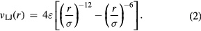
The minimum value of  is
is  , which is found at
  (compare figure 2). Commonly simulated simple liquid models are: the LJ pair potential (sometimes cut off at the minimum [40], sometimes with other exponents than 12 and 6), the purely repulsive inverse-power law (IPL) pair potentials
  [41, 42], the Yukawa 'screened Coulomb' pair potential
  [43–45], the Morse pair potential that is a difference of two exponentials [46, 47], and the HS pair potential (section 3).

Figure 2. The Lennard-Jones (LJ) pair potential defining the most widely studied liquid model system (equation (2)). This pair potential is a sum of two inverse-power-law terms, a harshly repulsive term with exponent 12 and a softer, attractive (negative) term with exponent 6. The LJ potential has been studied extensively in its pure form, but it also serves as a building block of many intermolecular model potentials, including those describing interactions between biomolecules.
Download figure:
Standard image High-resolution imageThe standard computer simulation method termed 'molecular dynamics' solves Newton's equations of motion numerically. If  is the force on particle i with mass mi, molecular dynamics traces out particle trajectories by solving a time-discretized version of Newton's second law,
  [1, 48–50]. Typical time steps are of order one femtosecond (10−15 s) in real units, so a sizable amount of computing power is required for getting accurate results (in particular for highly viscous liquids). For instance, simulating 1000 LJ particles for the equivalent of one millisecond requires about 1012 time steps, which takes more than a year on a state-of-the art GPU-based computer [51].
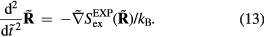
Newtonian dynamics conserves the energy E. When considered at constant volume V and particle number N, this is referred to as NVE dynamics. Nowadays it is more common to use NVT dynamics, which maintains a predefined temperature by modifying Newton's second law in a clever way [48, 49, 52]. For most quantities, including spatial and time autocorrelation functions, this method gives the same results as for NVE simulations. It is also possible to use NVU dynamics, which traces out a geodesic curve on the constant-potential-energy hypersurface [53], leading to the same results as NVE or NVT dynamics [54]. Constant-pressure (NPT) dynamics is an option that is popular, in particular, among chemists and material scientists because experiments usually take place at ambient pressure.
The above dynamics are all deterministic, i.e. once set into motion the system's path is in principle uniquely determined. An alternative is the so-called Brownian or Langevin stochastic dynamics. For details about such dynamics the reader is referred to the literature [48]; we here just note that deterministic and stochastic dynamics give the same static—and in most cases also very similar dynamic—properties [54–56].
3. The hard-sphere paradigm
This section summarizes the liquid-state paradigm according to which any simple liquid may be modeled by the HS system. This picture is built on the idea that liquid behavior dominated by excluded-volume effects is modeled in the most economic way by the HS system [1].
3.1. The van der Waals picture of liquids
Two isolated, uncharged atoms or molecules do not interact when they are far from each other. Approaching one another, a regime of weak attractions is entered caused by the so-called van der Waals forces [57]. These basically reflect the fact that electronic wave functions can lower their energy by spreading over a larger volume. When the distance becomes comparable to the atomic/molecular size, strong repulsions appear deriving ultimately from the Fermi statistics of the electrons. This is why it is almost impossible to compress a liquid or a solid.
The idea of classifying forces into repulsive and attractive goes back in time at least to 1755 in which the famous philosopher Kant proposed that, fundamentally, there are only these two kinds of forces with which one point of matter can impress motion on another [58]. In 1873 van der Waals transformed this picture into a quantitative theory by basing his equation of state upon it [2, 16]. The modern van der Waals picture may be summarized as follows [1–8, 59]. The strongly repulsive forces imply that a liquid's atoms or molecules cannot approach one another below a certain distance, a distance that depends slightly on the temperature because at high temperature more kinetic energy is available for overcoming the repulsive forces. These forces thus give rise to severe constraints on the particles' motion. The attractive forces, on the other hand, do not really have any effect on structure and dynamics because they merely contribute a negative, density-dependent but spatially virtually constant potential. As stated eloquently by Hansen and McDonald [1]: '...the structure of most simple liquids, at least at high density, is largely determined by the way in which the molecular hard cores pack together. By contrast, the attractive interactions may, in a first approximation, be regarded as giving rise to a uniform background potential that provides the cohesive energy of the liquid but has little effect on its structure. A further plausible approximation consists in modeling the short-range forces by the infinitely steep repulsion of the hard-sphere potential'. The van der Waals picture works best for liquids of atoms or roughly spherical molecules that are not bonded to each other by covalent or hydrogen bonds [1], the so-called nonassociated liquids. In the words of Chandler [60], the intermolecular structure of a nonassociated liquid 'can be understood in terms of packing. There are no highly specific interactions in these systems'. In contrast, water is an example of an associated liquid, and its 'linear hydrogen bonding tends to produce a local tetrahedral ordering that is distinct from what would be predicted by only considering the size and shape of the molecule'.
What is henceforth referred to as the hard-sphere paradigm is the assumption that, to a good approximation, any simple liquid with strongly repulsive forces may be modeled as a system of hard spheres. This idea has dominated liquid-state research for many years, in particular after the 1960s when it first got convincing support from computer simulations. Extensive research since then has demonstrated that, based on the HS system as the zeroth-order approximation, it is possible to construct highly successful perturbation theories for, e.g. a liquid's thermodynamics and pair distribution function (the probability to find two particles a certain distance apart relative to that for a system of random particles at the same density) [1, 7, 40, 61–65].
3.2. The hard-sphere system
Figure 3 shows coexisting liquid and solid phases of the LJ system (equation (2)). Each LJ particle is represented by a sphere, i.e. as a HS particle defined by having infinite pair potential when the pair distance r obeys  (
( is the particle radius) and zero potential otherwise. This representation makes good sense, because the quasiuniversality of structure discussed below implies that the structures of the LJ and HS systems are virtually identical.

Figure 3. Snapshot of coexisting phases of the LJ system in which each particle is represented by a sphere (reproduced with permission from [66]; copyright 2013 AIP Publishing). Due to quasiuniversality, the hard-sphere (HS) system of freely moving spheres represents the LJ system well; for instance, the relative particle positions of the HS system are close to those of the LJ system and most other simple liquids (section 4). Above the packing fraction 0.545 the equilibrium structure of the HS system is a face-centered cubic crystal. The HS crystal is thermodynamically stable at high packing fraction because it has higher entropy (but same energy) compared to that of the same-density, same-temperature liquid. This results in a lower free energy.
Download figure:
Standard image High-resolution imageHS particles have no rotational degrees of freedom and move in straight lines with constant velocity until they collide elastically, i.e. by conserving momentum and (kinetic) energy. At low density the HS system is gas like, at higher density it is liquid like, and at the highest densities it is crystalline [67, 68]. Using instead Brownian (stochastic) dynamics [48], which neither conserves momentum nor energy, leads to identical results for the static distribution functions and to very similar time-autocorrelation functions [56].
For a system of N HS particles in volume V one defines the packing fraction ϕ as the occupied fraction of the total volume, i.e.
The largest possible packing fraction is that of the face-centered cubic crystal in which  , a result known as 'Kepler's theorem' [69]. For many years this was 'known by all physicists and greengrocers, and conjectured to be true by most mathematicians...', but eventually Kepler's theorem was proven rigorously [70].
Above the packing fraction 0.492 the equilibrium HS system is partly crystalline, and for  it is fully crystallized [33, 71, 72]. By applying a finite rate of compression it is possible to overcompress the liquid HS system to higher packing fractions than 0.545, just as real-life liquids may be supercooled below their freezing point [73–78]. In the metastable, overcompressed state the HS system's viscosity increases dramatically as a function of density, and the system eventually jams into a glass phase in which only localized vibrational-type motion survives [69], [79–81].
Like the ideal-gas model or the Ising model for magnetism, the HS model is widely regarded as the idealized model liquid [1, 68]. In mathematics, the HS system has been studied for centuries. More recently, the problem of packing spheres densely in d dimensions became of interest to computer scientists because of its importance for coding theory in communication [82]. In physics, the HS model is receiving renewed interest these years [69, 83, 84]; for instance it was recently solved exactly in infinite dimensions in a tour-de-force replica calculation [81]. The HS model is also the generic model for studies of jamming [69, 79, 83, 85], a field in which the last decade has brought significant advances based, in particular, on the notions of isostaticity and marginal stability [80], [86–90].
3.3. Reduced units
According to the HS paradigm any simple liquid with strongly repulsive forces corresponds to a HS system. This implies that any two such liquids must have very similar properties at two thermodynamic state points that map onto HS systems with the same packing fraction. We refer to this as the HS explanation of quasiuniversality. But what is meant by 'very similar properties'? In the present context this means very similar structure and dynamics when these are made dimensionless using proper units; in contrast, the thermodynamic equations of state connecting temperature, density, and pressure generally differ significantly among quasiuniversal systems.
Which unit system should be used for characterizing quasiuniversality? Generalizing equation (2) any potential energy function  can be expressed in terms of an energy ε, a distance σ, and a dimensionless function
  , as follows

A 'microscopic' unit system may be defined based on the energy unit ε, length unit σ, and time unit  (m is the particle mass). Is this the right unit system to use in tests for quasiuniversality? Perhaps surprisingly, even though results of computer simulations are usually reported in these microscopic units, the answer is no.
Consider a simple liquid for which the two thermodynamic state points  and
and  are well modeled by HS systems with the same packing fraction. According to the HS paradigm and the van der Waals picture these two state points have the same reduced pair distribution functions
  . In particular, these function's maxima must be at the same value of
  . At a state point with density ρ the maximum nearest-neighbor distance scales with density as
  . Thus the proper length unit to use is that defined by the density:
  . Likewise, if the reduced velocity time-autocorrelation function
  is to be invariant, this must apply in particular to its zero-time value,
  . Since the kinetic energy scales in proportion to v2 and since
  by the equipartition theorem, the proper energy unit must be the thermal energy
  . In turn, via the particle mass and thermal average velocity this leads to the time unit
  . In summary, the HS paradigm implies that the correct units to use in relation to quasiuniversality are the following 'macroscopic' energy, length, and time units:

Note that these units are experimentally assessable, but state-point dependent. In contrast, the microscopic units ε and σ are state-point independent, but not experimentally assessable—in fact, by redefining the function  in equation (4) they can be based on any fixed energy and length.
Henceforth, whenever a quantity is referred to as 'reduced', it has been made dimensionless using the macroscopic units of equation (5). Reduced quantities are denoted by a tilde. For instance, if D is the diffusion constant,  .
.
4. Quasiuniversality
This section presents examples of simple liquids' quasiuniversal structure and dynamics. As mentioned, there is no exact universality; systems with different potentials are different [91]. In liquid state theory 'structural' quantities refer to averages of density equal-time spatial correlation functions, whereas 'dynamical' quantities more generally involve time-correlation functions and their time integrals as expressed, e.g., in transport coefficients. We start by looking at the former.
4.1. Structure
The simplest structural characteristic is the density spatial autocorrelation function. By neutron or x-ray scattering experiments one measures its Fourier transform, the so-called coherent scattering function  . If
. If  is the scattering vector and the system's N particles are located at the positions
  , the coherent scattering function is defined by
 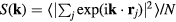 in which the sharp brackets denote a thermal average [1]. A crystal's
  has pronounced peaks at the reciprocal lattice vectors [29, 30], whereas for a liquid the peaks are broader and
  is independent of the direction of
  .
.
Figure 4(a) shows static structure factors of the HS (dots) and LJ (full curve) liquids based on almost 50 years old computer simulations [92]. The striking finding already at that time was that these quite different systems have very similar structure. Figure 4(b) shows the structure factor of IPL systems defined by  with exponents n ranging from 10 to 36, as well as that of the HS system (corresponding to the
  limit), all simulated close to freezing. Again there is approximate identity. Experiments show that simple liquids like molten metals [94] and inactive gases [95] have structure factors close to those of the HS system.

Figure 4. Structural quasiuniversality. (a) Static structure factor of the HS (dots) and LJ (full curve) liquids close to the triple point (based on simulation data of Verlet [92], reproduced with permission from [1]; copyright 2006 Elsevier). It is far from obvious that state points can be found where the structure factors of two such different systems are virtually identical. (b) Results close to freezing for IPL systems with exponents ranging from 10 to 36, as well as those of the HS system (black curve) (reproduced with permission from [93]; copyright 2009 American Institute of Physics).
Download figure:
Standard image High-resolution image4.2. Dynamics
Experimental signatures of dynamic quasiuniversality have been obtained for molten metals and inactive gases. In the latter case, the half width of the coherent inelastic scattering factor follows the prediction of the HS model solved in the so-called Enskog theory [97]. The dynamics of liquid Gallium likewise follows the Enskog prediction [98]. Experimental data for the self-diffusion constant and viscosity of certain small-molecule liquids like methane and ethane have also been interpreted successfully in terms of the HS model [99], thus establishing experimental quasiuniversality for the dynamics.
Computer simulations have documented dynamic quasiuniversality in greater detail [42, 56, 96], [100–102]. Figure 5(a) shows the inverse diffusion constant as a function of the HS packing fraction  determined by fitting the given system's static structure factor to that of a HS system. The figure shows data for different LJ-type systems simulated with both Newtonian and Brownian dynamics. Figure 5(b) shows similar results, including here also experimental data for a clearly non-quasiuniversal pair-potential system. Figure 5(c) shows the product of diffusion constant and viscosity for IPL systems (
 ) plotted as a function of 1/n; the lower data set refers to this product in reduced units, demonstrating quasiuniversality.
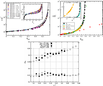
Figure 5. Dynamic quasiuniversality. (a) Inverse diffusion constant as a function of the HS packing fraction determined for each system by fitting its static structure factor to that of the HS system (black circles); the full curve is a theoretical prediction. Data are given for LJ-type systems with different exponents for both Newtonian and Brownian dynamics; the inset shows the same quantity in a different unit system (reproduced with permission from [56]; copyright 2013 American Physical Society, which gives details of the systems studied). The figure shows that systems with similar structure have similar dynamics. (b) A figure like that in (a) in which 'microgels' and 'dendrimers' refer to experimental data. This figure emphasizes that not all liquids are quasiuniversal (reproduced with permission from [96]; copyright 2011 American Physical Society, which gives details of the systems studied). (c) Product of the diffusion constant and the viscosity for different IPL systems of different particle numbers at state points with the same structure (reproduced with permission from [42]; copyright 2007 Royal Society of Chemistry). The product is plotted as a function of the inverse IPL exponent; the lower part of the figure gives the product in reduced units for which it is approximately independent of the exponent, consistent with quasiuniversality of the dynamics.
Download figure:
Standard image High-resolution imageOne defines the so-called excess entropy of a system as the entropy minus that of an ideal gas at the same density and temperature (appendix). Note that since the ideal gas is maximally disordered, the excess entropy is negative. In 1977 Rosenfeld pointed out that the excess entropy of a simple liquid, Sex, in simulations determines the reduced diffusion constant and the reduced viscosity [103]. He justified this by arguing as follows. A thermodynamic state point of the HS system is characterized by the packing fraction ϕ (temperature merely scales the particle velocities). In particular, ϕ determines Sex. Thus if two systems at two state points are well described by HS systems with the same packing fraction, they have the same excess entropy. For such systems the excess entropy determines the reduced-unit dynamics in a quasiuniversal way. By reference to Enskog theory Rosenfeld in 1999 interestingly managed to extend excess entropy scaling to the gas phase [104], but our focus below remains on the condensed 'ordinary' liquid phase.
Excess-entropy scaling did not receive a great deal of attention until about the year 2000, although a closely related two-particle entropy scaling was discussed briefly in 1996 by Dzugutov [108]. By now many systems, primarily in computer simulations, have been shown to conform to excess-entropy scaling [109–112]. Examples are given in figure 6, which in (a) shows numerical data for several systems. This figure also presents data for three exotic systems not obeying excess-entropy scaling revealed as an absence of data collapse; the two left-hand figures demonstrate quasiuniversal excess-entropy scaling for IPL systems. Other simple liquids like the LJ or the Yukawa (screened Coulomb) systems have reduced diffusion constants that fall virtually on top of the IPL data when plotted as functions of the excess entropy [103]. Figure 6(b) shows the reduced viscosity and diffusion constants for IPL systems as a function of the two-particle entropy, a quantity that gives the dominant contribution to Sex. Figure 6(c) presents experimental data for nitrogen at various temperatures and pressures.

Figure 6. Excess-entropy scaling. (a) Simulations of the diffusion constant with the four lower figures giving this quantity in reduced units for different models (reproduced with permission from [105]; copyright 2011 Royal Society of Chemistry, which gives details of the systems studied). The left pair of figures gives data for IPL systems of different exponents (n = 8–36), clearly conforming to excess-entropy scaling. The remaining figures give data for three systems violating excess entropy scaling, demonstrating that quasiuniversality has exceptions. (b) Reduced diffusion constant (upper figure) and reduced viscosity (lower figure) as functions of the two-particle entropy for IPL systems of different exponents (n = 4–36) (reproduced with permission from [106]; copyright 2015 Royal Society of Chemistry). Since the two-particle excess entropy gives the most important contribution to the excess entropy, this figure confirms IPL quasiuniversality. (c) Experimental data for the reduced viscosity of liquid nitrogen plotted as a function of minus the excess ('reduced residual') entropy at pressures up to 10 GPa (reproduced with permission from [107]; copyright 2014 American Chemical Society).
Download figure:
Standard image High-resolution image4.3. Thermodynamics
Important features of simple liquids' thermodynamics are not quasiuniversal, for instance the equation of state connecting temperature, pressure, and density. There are some thermodynamic quasiuniversalities, however. One of these relates to the constant-volume specific heat CV's temperature variation. As noted by Rosenfeld and Tarazona [103, 114], simple liquids obey  to a good approximation at constant density. Figure 7 gives computer simulation data confirming this. While the figure also includes simulation data for non-simple liquids like water, inspection reveals that the Rosenfeld–Tarazona relation works best for the LJ and IPL systems.

Figure 7. Excess isochoric specific heat for several models plotted as a function of T −2/5 at constant density in order to allow for a comparison to the Rosenfeld–Tarazona prediction  (reproduced with permission from [113]; copyright 2013 American Institute of Physics, which that gives details of the systems studied). The orange lines are best fit power laws; when these lines are straight, the Rosenfeld–Tarazona relation is obeyed. The figure includes data for molecular models, as well as experimental data for supercritical argon (inset). The Rosenfeld–Tarazona relation is seen to work fairly well for all systems, but best for the single-component Lennard-Jones (SCLJ) and IPL pair-potential liquids.
Download figure:
Standard image High-resolution imageInteresting thermodynamic quasiuniversalities have been reported going beyond the condensed liquid phase in focus here. These involve, e.g. the liquid-vapor coexistence region [115, 116], the so-called Zeno line [117], the behavior of supercritical fluids [118], and the existence of generalized corresponding-states equations [116, 119].
4.4. The freezing and melting transitions
Quasiuniversality applies also for crystallization and melting [120–127]. Figures 8(a) and (b) show data for the structure factor of iron at ambient and high pressure along the freezing line. Invariance of the structure along the freezing line is demonstrated in (b) reporting reduced-unit structure factor data for iron at freezing up to a pressure of 58 GPa. This case is important because the Earth's core consists largely of molten iron [128–130]. Figure 8(c) gives the reduced viscosity of fifteen metallic elements plotted as a function of melting temperature over temperature. Clearly these metals behave very similarly. In particular, the reduced viscosity is quasiuniversal at freezing [131–133].

Figure 8. Experimental data illustrating liquids' quasiuniversality close to freezing. (a), (b) Structure factor of liquid iron along the freezing line up to pressures found far inside the Earth [130] (reproduced with permission from [134]; copyright 2004 American Physical Society). As shown in (b) the structure is approximately invariant as a function of the reduced wavevector  . The full curves in (a) are HS structure factors, the full red curve in (b) is iron's structure factor at ambient pressure. (c) Natural logarithm of the reduced viscosity of fifteen metals plotted as a function of melting temperature over temperature, demonstrating quasiuniversality (reproduced with permission from [135]; copyright 2005 Carl Hanser).
Download figure:
Standard image High-resolution imageFreezing and melting of simple systems are characterized by several quasiuniversal properties [123, 127], for instance the following:
- 1.
- 2.A liquid freezes when the maximum of its structure factor exceeds a quasiuniversal value close to, but slightly below 3 [138] (the Hansen–Verlet criterion).
- 3.
- 4.
- 5.
- 6.


4.5. Defining quasiuniversality
The HS paradigm makes it possible to give a precise definition of quasiuniversality. Consider two systems at two thermodynamic state points. If the systems are here described by HS systems with the same packing fraction, all reduced-unit quantities referring to structure and dynamics of the two systems are identical to a good approximation. In practice one does not know the HS packing fraction, but this inspires to the following characterization of quasiuniversality:
- If two systems have in common a single reduced-unit quantity characterizing structure or dynamics at two—possibly different—thermodynamic state points, all other reduced-unit structural or dynamical quantities at these state points are also identical to a good approximation.
The above property defines an equivalence relation among liquids. There could be more than a single equivalence class (which we in section 8 suggest is the case for mixtures), but the focus below is on the large equivalence class of single-component systems that includes the HS system, the LJ and related systems, the IPL systems, and the Yukawa system. As we shall see, this class also includes the purely repulsive exponential pair potential, as the most prominent member in a certain sense.
5. Challenges to the hard-sphere paradigm
In the van der Waals picture any simple liquid is well represented by a HS system. This explains quasiuniversality, which was confirmed by the numerical and experimental data presented in the last section, implying that the present liquid-state paradigm works well, right? This is undoubtedly the case. Nevertheless, there are a few challenges to the HS paradigm:
- Physically and formally. The HS system consists of particles moving most of the time according to Newton's first law, i.e. along straight lines with constant velocity, until collisions instantaneously change their velocities to new, constant values. In any realistic liquid model and for any real liquid each particle is kept in check by fairly strong forces from its several (10–14) nearest neighbors. Given this difference, how can one understand why so many simple liquid's structure and dynamics are close to those of the HS system? Moreover, the HS system is non-analytic with a discontinuous potential-energy function. It would be nice to be able to explain quasiuniversality in terms of an analytical reference system.
- Operationally. How to determine the effective HS packing fraction of a given simple liquid at a given state point? The literature gives many different answers to this question, for instance those of [99], [145–152]. The simplest of these criteria determines the effective HS radius from the equation
 [150], but after half a century of research there is still no recipe for calculating the HS packing fraction that is generally agreed upon. Why is this so difficult? Perhaps it reflects the following more fundamental problem:
 - Exceptions. The van der Waals picture is not able to predict which systems are quasiuniversal and which are not. It is not surprising that complex liquids like water violate quasiuniversality [12, 20], [153–157]. But even some simple liquid models (i.e. pair-potential systems) with strong repulsive forces have highly complex behavior [158], although according to the HS paradigm this should not be the case. Examples of non-quasiuniversal simple systems are the Gaussian core model and the Jagla ramp-type potential models, both of which have water-like anomalies in parts of their thermodynamic phase diagram [35, 36, 159]. Thus in parts of their phase diagram these models exhibit the anomalies of density increasing upon isobaric heating, the diffusion constant increasing upon isothermal compression, melting instead of freezing upon isothermal compression, etc.

Which property of the HS system is crucial for deriving quasiuniversality? The HS explanation of quasiuniversality hinges on the fact that the HS system's reduced-unit structure and dynamics are determined by a single number, the packing fraction. This property makes the HS system's phase diagram effectively one-dimensional in regard to structure and dynamics. This implies quasiuniversality according to the definition given in section 4.5 because any reduced-unit structural or dynamical quantity identifies the corresponding HS system's packing fraction, which in turn determines all of structure and dynamics. In particular, any quasiuniversal liquid is predicted to have lines in its thermodynamic phase diagram along which structure and dynamics are (virtually) invariant in reduced units.
An alternative explanation of quasiuniversality should preferably retain this feature. The concept of packing fraction is unique to the HS system, of course, but since the packing fraction determines the excess entropy Sex, an obvious candidate for the lines in the phase diagram of invariant structure and dynamics are the configurational adiabats, i.e. the lines defined by 
6. The exponentially repulsive pair potential and quasiuniversality
This section presents an alternative to the HS justification of simple liquids' quasiuniversality [160]. Sections 6.2– 6.4 are a bit technical, but all necessary information is provided for verifying the calculations carried out.
6.1. The system

The  potential is the purely repulsive pair potential defined by

Born and Meyer already in 1932 used an exponentially repulsive term in a pair potential [161], justifying it from the fact—at that time recently established—that electronic bound-state wavefunctions decay exponentially in space. There are only few studies of the pure  system in the literature; usually an
  term appears in tandem with an r−6 attractive term [161, 162] or multiplied by a 1/r term as in the Yukawa 'screened Coulomb' pair potential [43, 163, 164]. Kac and coworkers used a HS pair potential minus a long-ranged
  term for rigorously deriving the van der Waals equation of state in one dimension [165].
Like any other purely repulsive system, the  system has a well-defined freezing transition, but no liquid-vapor transition—there is just a single fluid phase. The density-temperature phase diagram of the
  system is shown in figure 9(a), in which the full black line covers the solid–liquid coexistence region. The colors reflect the virial potential-energy (Pearson) correlation coefficient R defined by
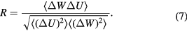
Figure 9. The  system defined by equation (6) [160]. (a) Temperature-density thermodynamic phase diagram with temperature in units of
  and density in units of
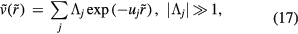
  . The color coding gives the virial potential-energy correlation coefficient R (equation (7)). Three isomorphs are indicated with black dashed lines (see section 6.2). The freezing and melting lines are both isomorphs to a good approximation [166]; the solid black line covers the liquid–solid coexistence region. (b) Potential energies U2 of 20 configurations, each taken from an equilibrium simulation at the state point
  and subsequently scaled uniformly ±20% up and down in density. At each density the average of the 20 scaled configurations' potential energy was subtracted and the energies subsequently scaled to unit variance. If the curves rarely cross, which is the case here but not for all systems, the scaling inequality equation (8) is obeyed to a good approximation, which ensures the existence of isomorphs. (c) Time development of the normalized virial and potential energy equilibrium fluctuations at the same state point as (b), confirming the existence of strong correlations.
Download figure:
Standard image High-resolution imageHere  denotes deviation from the equilibrium value and the sharp brackets are constant-volume canonical averages; recalling that
  is the configuration vector and
  the potential energy, the virial function is defined by
  (the average virial W determines the pressure via the identity
  [1, 48, 167]).
We see from figure 9(a) that the  system has strong WU correlations in the low-temperature part of its phase diagram. This is where
  , implying that the finite value of
  is of no significance because zero particle separation is highly unlikely. Systems with R > 0.9 were initially referred to as 'strongly correlating' [168], but that term was repeatedly confused with strongly correlated quantum systems and instead the term R (Roskilde) simple is now sometimes used [107], [169–176]. As shown in the next section, R systems are simple because in regard to structure and dynamics they have, just like the HS system, an essentially one-dimensional thermodynamic phase diagram.
6.2. Isomorphs
The ' explanation' of quasiuniversality given in section 6.3 below makes use of the theory of isomorphs [38, 166]. Independent of quasiuniversality, isomorphs are lines in the thermodynamic phase diagram of certain systems along which structure and dynamics in reduced units are invariant to a good approximation. Real-world liquids and solids with isomorphs are believed to include most metals and van der Waals bonded molecular systems, but exclude most covalently or hydrogen-bonded systems [19, 177].
An isomorph is defined as a configurational adiabat, i.e. a curve with  , for any system characterized by the following scaling property [178]

Only for systems with a potential-energy that is a constant plus an Euler-homogeneous function is the above 'hidden-scale-invariance' identity rigorously obeyed. For the isomorph theory to work to a good approximation it is enough, however, that equation (8) applies for most configurations  and
and  , i.e. for most of the typical configurations.
Equation (8) is mathematically equivalent to the conformal-invariance condition  , which by differentiation with respect to λ implies for the virial function
  . Thus same potential energy implies same virial to a good approximation, so equation (8) implies strong correlations between the equilibrium fluctuations of W and U and that the correlation coefficient R of equation (7) is close to unity. Thus only R simple systems have isomorphs.
Figure 9(b) validates equation (8) for the  system by showing how properly normalized potential energies of 20 selected configurations change under uniform scaling—the figure is constructed such that whenever the curves do not cross, equation (8) applies. Figure 9(c) shows how the virial and potential energy of the
  system fluctuate strongly correlated over the course of time. In summary, figure 9 shows that
  system is R simple in the low-temperature part of the phase diagram [160].
What are the characteristic properties of R systems? Following the Landau and Lifshitz theory of entropy fluctuations [179], one can define a microscopic excess entropy function by 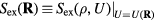 in which
  is the thermodynamic excess entropy of the state point with density ρ and average potential energy U [178]. By inversion, the potential-energy function obeys
  in which
  is the thermodynamic average potential energy as a function of density and excess entropy.
The above definition is completely general. Consider now a system obeying equation (8) and suppose that  is a configuration of density
  with the same reduced coordinate as
  , a configuration of density
  , i.e.
  (compare the definition of reduced units equation (5)). It follows from the microcanonical expression for the excess entropy (appendix) that if 'Vol' is the reduced-coordinate configuration-space volume, one has
  and
and  . Applying
  to the inequality of the first set, we see that the two sets are identical since equation (8) works 'both ways'. This means that
  depends only on the configuration's reduced coordinate
  , implying that

Since the thermodynamic excess entropy Sex at any given state point is the average of the microscopic excess entropy function,  , equation (9) implies invariant structure and dynamics along the isomorphs [178]. To show this in detail, note first that in the reduced unit system defined by equation (5) Newton's second law is
  in which the reduced force
  is defined from the full 3N-dimensional force vector
  by
by  . Since
  , equation (9) implies
  . Because
  (appendix) this means that
Equation (10) implies that the reduced-unit dynamics is invariant along the isomorphs. Since structure is found by averaging over the equilibrium time development, the reduced-unit structure is also isomorph invariant.
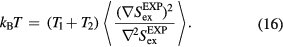
How to map out the isomorphs in the phase diagram? Calculating Sex at a given state point is possible, but tedious. One can avoid this and identify the curves of constant Sex by utilizing the fluctuation identity  [166]. For instance, if the right-hand side is five at a certain state point, for a one percent density increase one stays on the same isomorph by increasing temperature five percent. The fluctuation identity was used in this way to step-by-step identify the isomorphs of figures 9(a) and 10. Another method for tracing out isomorphs utilizes equation (12) derived below, which for any two configurations at different densities with the same reduced coordinates,
  and
and  , implies
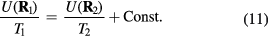
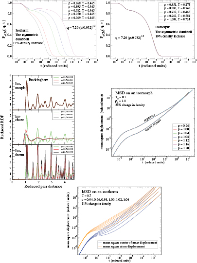
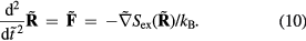
Figure 10. Examples of applications of the isomorph theory to other systems than simple liquids, demonstrating that invariance of the reduced-unit structure and dynamics along isomorphs is not limited to simple, quasiuniversal systems. (a), (b) Incoherent intermediate scattering function for the center of mass of the asymmetric dumbbell model consisting of two different-sized LJ spheres connected by a rigid bond (reproduced with permission from [180]; copyright 2012 American Chemical Society). The figures compare results along an isotherm and an isomorph, demonstrating isomorph invariance of the dynamics for this molecular system. (c) Radial distribution functions (RDFs) for a face-centered cubic crystal of particles interacting via the so-called Buckingham pair potential consisting of an exponentially repulsive term and an r−6 attractive term [161, 162] (reproduced with permission from [181]; copyright 2014 American Physical Society). The upper figure shows results for three isomorphic state points; for comparison the two lower figures give results obtained by varying only temperature and density, respectively. Clearly isomorph invariance of structure is not limited to liquids. (d), (e) Mean-square displacement (MSD) for the 10-bead flexible Lennard-Jones chain model, a primitive polymer model in which each molecule consists of ten LJ particles bonded with rigid but freely rotating bonds (reproduced with permission from [182]; copyright 2014 American Institute of Physics). (d) shows the MSD along an isomorph for the segments and center of mass, (e) shows the same quantities along an isotherm for less than half the density variation.
Download figure:
Standard image High-resolution imageHere T1 and T2 are the temperatures of the state points at which the two configurations are typical equilibrium configurations. Equation (11) implies the same canonical-ensemble probability of the configurations  and
and  , which was the original isomorph definition [166]. In experiments, for any R simple system isomorphs may be identified with the lines of constant reduced viscosity or diffusion constant [19]; for highly viscous liquids the isomorphs are basically the lines of constant relaxation time, the so-called isochrones [76, 170], [183–185].
In the next section the isomorph theory is used to derive quasiuniversality for a large class of simple liquids. The theory is not limited to such systems, however. To illustrate this we show in figures 10(a) and (b) the incoherent intermediate scattering function as a function of reduced time for a molecular model along an isotherm and an isomorph respectively, demonstrating isomorph invariance of the dynamics. Figure 10(c) shows results for the pair correlation function of a crystal evaluated along an isomorph, an isochore, and an isotherm [181]. Figures 10(d) and (e) show results for a simple polymer model, again demonstrating isomorph invariance of the dynamics.
Other applications of the isomorph theory beyond the realm of simple liquids include, for instance, rationalizing simulations of non-linear shear flows and zero-temperature plastic flows of glasses [186, 187]. Several well-known melting line invariants like the Lindemann ratio may also be understood in terms of the isomorph theory, because the melting and freezing lines are both isomorphs to a good approximation [166].
6.3. The family and quasiuniversality class

Figure 9 demonstrated that the  system obeys equation (9) well in the low-temperature part of the phase diagram. Expanding equation (9) to first order at a state point with excess entropy Sex and average potential energy U leads to
  (recall that
  ). In terms of the excess Helmholtz free energy
  , if the
  system's microscopic excess entropy function is denoted by
  , one thus has

The  system's reduced-unit dynamics is given by equation (10),
We proceed to show that a sum of two  systems from the low-temperature part of the phase diagram defines a system that also obeys equation (13). This fact is the basis for defining below the
  'family' of quasiuniversal pair potentials. Consider two systems,
  and
and  , obeying
  and
and  at the respective state points of some configuration
  . The systems' dynamics are both described by equation (13), and equation (12) implies
  as well as
 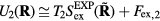 . For the 'sum' system defined by the pair potential
  one has
  , i.e.

in which  . This implies for the force vector

To show that the dynamics of the sum system is also described by equation (13) we first note that  , in which T is the temperature of the sum system state point at which the configuration
  is a typical equilibrium configuration. This is shown by making use of the configurational temperature identity
 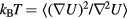 [179, 188], which via equation (14) implies
On the other hand, substituting  into the configurational-temperature identity leads to
  , i.e.
  . Thus equation (16) implies the required
  . Since the reduced force is defined by
  , we conclude from equation (15) that
  . This shows that the sum system's equation of motion is also equation (13) (compare equation (10)).
The above generalizes to an arbitrary sum of  terms and, in fact, also to a difference of such systems if thermodynamic stability is maintained [189, 190]. In order to state a precise (sufficient) condition for quasiuniversality of a system with pair potential
 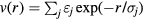 , we switch to reduced units. Defining the dimensionless numbers
  and
and  and noting that the condition
  translates into
  , if the reduced pair potential of a system at the state points of interest is given by
the system obeys equation (13). In particular, any sum or product of two pair potentials that can be written as in equation (17) with all  gives a pair potential that also obeys equation (13). Note that for equation (13) to apply it is not enough that the pair potential can be written as a superposition of exponentials with large coefficients—the 'wavevectors' uj cannot be so closely spaced that large positive and negative terms almost cancel one another, because that would effectively result in a term that does not have a numerically large prefactor [160].
Thus any system for which  at the state point in question can be approximated as in equation (17) with ujs that are not too closely spaced has the same dynamics as the
  system to a good approximation. Such systems are quasiuniversal in the sense of section 4.5, because knowledge of a single number characterizing the reduced-unit structure or dynamics is enough to identify Sex and thereby, via equation (13), all other reduced-unit structure and dynamics.
Having in mind the definition of quasiuniversality of section 4.5, the class containing the  pair-potential system will be referred to as the '
 quasiuniversality class'. It follows from the above that whenever equation (17) applies to a good approximation for a given pair-potential system (at the state points of interest), this system is in the
  quasiuniversality class. It is an obvious conjecture that the
  quasiuniversality class does not include other regular pair-potential systems, but at this point there is no proof of this. It is likely that the
  quasiuniversality class contains also non-pair-potential systems, however (section 8 proposes that this is the case). In view of the above we shall refer to pair-potential systems obeying equation (17) (with not too closely spaced ujs) as members of the '
 family'.
In summary, any member of the  family obeys equation (13) and is consequently in the
  quasiuniversality class. The HS system is in the
  quasiuniversality class, but not a member of the
  family because it does not obey equation (13). Finally, there may very well exist also non-pair potential members of the
  quasiuniversality class but these are by definition not in the
  family.
6.4. Examples
The numerical data presented in section 4 show that the IPL systems,  , are quasiuniversal. How would one justify this from the above [160]? Write first the reduced IPL pair potential in terms of the reduced radius
  as
as  with
with  . The well-known identity
  implies
 ![${{\tilde{{v}}\,}_{n}}\left(\tilde{{r}}\,\right)=\left[{{\Gamma}_{n}}/(n-1)!\right]{\int}_{0}^{\infty}{{u}^{n-1}}\exp \left(-u\tilde{{r}}\,\right)\text{d}u$](https://content.cld.iop.org/journals/0953-8984/28/32/323001/revision1/cmaa2565ieqn171.gif) . Discretizing the integral leads to
. Discretizing the integral leads to ![${{\tilde{{v}}\,}_{n}}\left(\tilde{{r}}\,\right)\cong \left[{{\Gamma}_{n}}/(n-1)!\right]\,\Delta u\,{\sum}_{j=0}^{\infty}{{\left((\,j+1/2)\Delta u\right)}^{n-1}}$](https://content.cld.iop.org/journals/0953-8984/28/32/323001/revision1/cmaa2565ieqn172.gif)
 . If one writes
  as
as ![$\exp \left[(n-1)\ln \left((\,j+1/2)\Delta u\right)\right]$](https://content.cld.iop.org/journals/0953-8984/28/32/323001/revision1/cmaa2565ieqn175.gif) , differentiation with respect to j shows that the dominant contributions to the sum come from the terms with
, differentiation with respect to j shows that the dominant contributions to the sum come from the terms with  . For typical nearest-neighbor distances one has
  , so the terms with
  are the most important ones. For these j's the prefactor of the exponential in the above sum is roughly
  . The largest realistic discretization step obeys
  . Thus for values of n larger than about 3 − 4, equation (17) is obeyed unless
  is very small, a condition that applies for the state points that have typically been studied [98], [191–194]. It follows that the IPL pair potentials are generally in the
  family, but that quasiuniversality is expected to gradually break down when n decreases and, in particular, goes below 3–4 [160] (note that for n < 3 there is no thermodynamic limit because the integral
  diverges). The gradual breakdown of quasiuniversality as the exponent is lowered is consistent with the finding that the crystal structure changes from face-centered cubic to body-centered cubic as n goes below 7 [195]. The one-component plasma [196], the n = 1 case of a Coulomb system of identical particles in a charge-compensating background, is not in the
  family (although it interestingly does obey excess-entropy scaling [103]).
Adding or subtracting two pair potentials in the  family defines a new system in the EXP family as long as the condition
  is obeyed for all j and the resulting ujs are not close to one another. An example is the LJ pair potential equation (2) at the liquid state point defined by
  and
and  . In terms of the reduced IPL functions introduced above, since
  at this state point, we have here
  . This is of the form equation (17), implying quasiuniversality of the LJ liquid at that state point. Similar arguments may be applied for LJ-type systems with exponents different from 6 and 12, but if the two exponents are close, a more detailed investigation is required because one may run into the problem of having close ujs. The Yukawa pair-potential system is quasiuniversal in much of its phase diagram [45].
We finally note an alternative connection to the HS system. As shown by Brito and Wyart the HS system's interactions are described in a mean-field, i.e. time-averaged, sense by the continuous pair potential  in which
  is the sphere diameter (
 for r < d) [88]. This may be rewritten
  , which at high packing fractions is a sum of quasiuniversal IPL terms because here
  and consequently the large n terms dominate.
7. The HS challenges revisited
Having established quasiuniversality for systems in the  family defined by equation (17) and shown that this includes the standard examples of quasiuniversal simple systems, one may ask to what degree using the
  system as reference system addresses the issues with the HS paradigm listed in section 5.
- Physically and formally. The HS system does not conform to equations (13) and (17) and is not a member of the family. On the other hand, the HS system is the limit of IPL pair potentials (). This suggests placing the HS system on the family's border (figure 11). In particular, the HS system has the same structure and dynamics as the family members, i.e. it is in the quasiuniversality class. In regard to the formal mathematics, all systems in the family have analytic potential-energy functions.
- Operationally. The problem that there is no unique method for determining the HS packing fraction of a quasiuniversal system at a given state point becomes irrelevant when the system is taken as the basic reference system.
- Exceptions. The Lennard-Jones Gaussian and the Jagla-type models, which are simple liquid exceptions to quasiuniversality [35, 36, 159], are not in the family as we shall see. It was conjectured above that all regular pair-potential systems in the quasiuniversality class are in the family, and if this holds true, it explains why these two systems are not quasiuniversal. They are not in the family because their pair potentials have Laplace transforms with no poles on the negative real axis, whereas any function in the form of equation (17) must have one or more such poles (it follows from the calculations of section 6.4 that, for instance, an IPL pair potential has all poles of its Laplace transform on the negative real axis).


Figure 11. Schematic representation of quasiuniversality according to the picture proposed in this paper. In the traditional explanation of quasiuniversality, two quasiuniversal systems have virtually identical reduced-unit structure and dynamics because they are both like the HS system; this argument places the HS system at center of the set of quasiuniversal systems. The above figure illustrates the set of members of the  family defined as the pair-potential systems that obey equation (17), exemplified by the systems A, B and C. These systems are all in the
  quasiuniversality class because they conform to the same equation of motion as the
  system, equation (13). In this picture the HS system lies on the border of the
  family because it is the
  limit of the r−n IPL systems (which explains the HS system's quasiuniversal structure and dynamics). The figure illustrates the two main points of this paper: (1) The EXP system may be regarded as the fundamental reference system from which simple liquids' quasiuniversality derives. (2) The HS system is not a regular member of the
  family of quasiuniversal systems. In this picture the fact that the HS system has quasiuniversal structure and dynamics is an effect of quasiuniversality, not its cause.
Download figure:
Standard image High-resolution image8. Outlook
The van der Waals picture has served liquid-state theory well for many years, in particular as the basis for highly successful perturbation theories [1, 7, 40], [62–65]. In regard to simple liquids' quasiuniversality there is also much to be learned from the van der Waals picture and the HS paradigm. The latter leads to the 'macroscopic' reduced units equations (5), which are essential for defining isomorphs, as well as to a precise definition of quasiuniversality (section 4.5). Moreover, the HS system provides the insight that quasiuniversality should be explained in terms of a reference system with a thermodynamic phase diagram that is basically one-dimensional in regard to structure and dynamics. Finally, the HS system points to the significance of the excess entropy for identifying the lines of virtually invariant structure and dynamics in the phase diagram [103]. Despite these several important points, the HS paradigm also has some challenges as we saw in section 5.
According to the van der Waals picture and the HS paradigm, the harsh repulsive forces determine the structure and dynamics of simple liquids implying that—to lowest order—these are well represented by a HS system. This cannot explain, however, why certain systems with strongly repulsive forces violate quasiuniversality, nor is it possible to predict a priori which simple systems are HS like and thus quasiuniversal, and which are not. The  family, on the other hand, consists of a well-defined class of systems (equation (17)), which all to a good approximation conform to the same equation of motion, equation (13), reflecting the fact that they basically have the same high-dimensional potential-energy surface. The degree to which this applies depends on how well the reduced pair potential can be represented as a finite sum of exponentials with large prefactors and how large these prefactors are.
A recent challenge to the HS paradigm relates to the underlying assumption that the repulsive and attractive pair forces play well-defined, separate roles for a liquid's physics [197–203]. The HS paradigm is a bit counterintuitive in this regard, in fact, because along the lines of constant HS packing fraction of a given system, the repulsive reduced forces change significantly. An illustration of this is given in figure 12(a), which shows Lennard-Jones pair potentials that all according to the isomorph theory at the given state point correspond to the same HS packing fraction. Inspecting these pair potentials, it is not obvious why they to a good approximation should have the same HS radius. They have the same structure and dynamics because the force on a given particle from its surrounding particles is almost the same (figure 12(b)). The take-home message is that it may be misleading to focus merely on the pair potential; there is a lot of cancellation going on when the individual pair forces are added as vectors to arrive at the force on a given particle, which after all via Newton's equations of motion is what determines the structure and dynamics.

Figure 12. Different Lennard-Jones pair potentials resulting in the same structure and dynamics to a good approximation (reproduced with permission from [197]; copyright 2013 IOP Publishing). (a) Different LJ pair potentials that according to the isomorph theory have virtually the same structure and dynamics at the state point  . In the van der Waals picture of quasiuniversality this is because these potentials' different repulsive forces are all represented by the same HS particle radius, i.e. at the state point in question each of the LJ systems in the figure is represented by a HS system with the same packing fraction. In the
  explanation of quasiuniversality, the different pair potentials define systems that conform to the same equation of motion, equation (13), reflecting the fact that these apparently quite different systems have basically the same high-dimensional potential-energy surface. (b) The x-components of the reduced-unit forces on a single particle coming from the different LJ potentials of (a) plotted as a function of time along a given trajectory, showing that the systems give rise to virtually the same forces and thus conform to the same equation of motion.
Download figure:
Standard image High-resolution imageThis paper focused on simple liquids' quasiuniversality. The corresponding crystals also have quasiuniversal structure and dynamics, although this remains to be investigated in detail. Just as for liquids, not all crystals are quasiuniversal or have isomorphs. A numerical study of crystals with and without isomorphs was recently published [181], compare figure 10(c).
There are a number of open questions relating to quasiuniversality, for instance the following:
- 1.Is there just one quasiuniversality class of single-component systems according to the definition proposed in section 4.5? Since the quasiuniversality class includes all well-known examples of quasiuniversality, we conjecture that the answer is yes [160]. Most likely, the situation is quite different for mixtures in which case each composition may have its own quasiuniversality class(es).
- 2.Are all single-component R simple systems, i.e. with strong virial potential-energy correlations, in the quasiuniversality class?
- 3.Do non-pair potential systems exist that obey the quasiuniversal equation of motion equation (13)? These might include potentials accurately describing molten metals; thus recent ab initio quantum-mechanical density-functional theory (DFT) simulations have shown that most liquid metals have strong virial potential-energy correlations close to the triple point [177], and the DFT-generated potentials are not pair potentials.
- 4.What it the origin of the Rosenfeld–Tarazona relation according to which the isochoric specific heat at constant density varies with temperature as to a good approximation? Can this be explained by reference to the pair potential?
- 5.What is the role of dimensionality? It was recently shown rigorously that all reasonable pair-potential systems obey hidden scale invariance (equivalent to equation (8)) in the limit of infinitely many dimensions [204], confirming a previous speculation [127]. In connection with the further intriguing finding of dynamic quasiuniversality in high dimensions [205], this suggests that simple liquids and their quasiuniversality should be understood in terms of a systematic 1/d expansion quantifying the deviations from quasiuniversality. Thus the elusive small number λ needed to circumvent the strong-coupling complexities in liquid-state theory (section 2.3) may simply be given by, with the yet-to-be constructed 1/d expansion converging more rapidly for R simple systems than for systems in general [127, 206]. In this view, the HS system may be regarded as the 'poor man's' limit of high dimensionality [206].
- 6.Do simplifications arise for quantum liquids of particles interacting with a pair potential belonging to the quasiuniversality class [207]?
- 7.


It appears that there is still a lot of work to do in this fundamental field of research.
Acknowledgments
The author wishes to thank T Hecksher, A K Bacher, and H Larsen for technical assistance in preparing the manuscript. This work was supported by the Danish National Research Foundation via grant DNRF61.
Appendix.: Excess thermodynamic quantities
This appendix is largely identical to the appendix of [178], but is repeated here in order to make the text self contained. Consider a system of N identical particles in volume V with number density  . The particles are represented by the 3N-dimensional configuration vector
  ; the corresponding reduced (dimensionless) configuration vector is given by
  . Below we review the definition of excess thermodynamic quantities and derive the following microcanonical expression for the excess entropy at the state point with density ρ and average potential energy U:
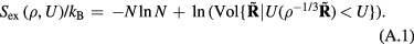
Here 'Vol' refers to the volume of the set in question, i.e. the  integral of the unity function over all configurations with potential energy lower than U.
If the momentum degrees of freedom are denoted by  ,
,  is the Hamiltonian, and
  , the Helmholtz free energy F is given [1] by
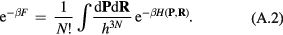
The Planck constant h and the indistinguishability factor  are conveniently absorbed by writing
  in which
  is the free energy of an ideal gas at the same density and temperature,
 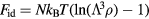 where
where  is the de Broglie wavelength (m is the particle mass) [1]. The excess free energy
  is thus given [1] by
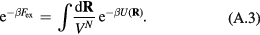
Due to the identity  , any thermodynamic quantity that is a derivative of F separates into an ideal-gas contribution and an excess contribution deriving from the particle interactions. For example,
  , the pressure is given by
  in which W/V is the excess pressure, the entropy S obeys
  in which
  , the isochoric specific heat CV separates into a sum of two terms, etc.
The excess entropy obeys  because any system is more ordered than an ideal gas at the same density and temperature. As temperature goes to infinity at fixed density,
  because the system approaches an ideal gas. The relation between excess entropy, potential energy, and temperature is the usual one, i.e.
This follows by subtracting from the textbook identity  the ideal gas case
  , leading to
  .
.
Proceeding to derive equation (A.1), recall that the Heaviside theta function  is unity for positive arguments and zero for negative. The volume of the set of configurations with potential energy less than U relative to the full configuration space volume VN is denoted by
  and given by
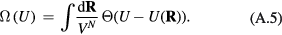
If Xi is one of the 3N particle coordinates and  , the microcanonical ('mc') average of
  is by definition given by
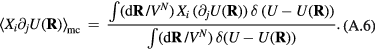
Following Pauli's derivation [208], via the fact that  and a partial integration we get for the numerator
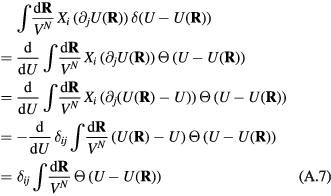

The denominator of equation (A.6) is  , so
, so
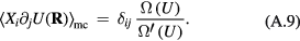
Next, the canonical ('can') average of  is calculated. If
  is the partition function we have
 . Via a partial integration this gives
  . Since averages are ensemble independent, equation (A.9) implies
Combined with equation (A.4) this means that  , i.e.

The a priori density-dependent integration constant C is determined from the boundary condition  for
for  . From equation (A.5) we conclude that C = 0 at all densities since
  as
as  . Rewriting finally the definition of
  as an integral over the reduced coordinate vector
  leads to equation (A.1).