


Abstract
Half-life measurements of radionuclides are undeservedly perceived as 'easy' and the experimental uncertainties are commonly underestimated. Data evaluators, scanning the literature, are faced with bad documentation, lack of traceability, incomplete uncertainty budgets and discrepant results. Poor control of uncertainties has its implications for the end-user community, varying from limitations to the accuracy and reliability of nuclear-based analytical techniques to the fundamental question whether half-lives are invariable or not. This paper addresses some issues from the viewpoints of the user community and of the decay data provider. It addresses the propagation of the uncertainty of the half-life in activity measurements and discusses different types of half-life measurements, typical parameters influencing their uncertainty, a tool to propagate the uncertainties and suggestions for a more complete reporting style. Problems and solutions are illustrated with striking examples from literature.
Export citation and abstract BibTeX RIS

Content from this work may be used under the terms of the Creative Commons Attribution 3.0 licence. Any further distribution of this work must maintain attribution to the author(s) and the title of the work, journal citation and DOI.
1. Introduction
The exponential decay of radionuclides as a function of time is a cornerstone of nuclear physics and radionuclide metrology. Since its discovery in 1903 by Rutherford and Suddy [1], it has been confirmed in numerous measurements of radioactive decay (see e.g. in [2]). Theoretical derivations of the exponential law can be achieved from probabilistic and quantum-mechanical points of view [3]. Both approaches imply that spontaneous nuclear transitions occur with a constant rate coefficient λ. At the level of single atoms, it is a stochastic process in which the survival time in a time period t is given by e−λt. For a set of atoms, the number of surviving and decayed atoms are ruled by a binomial distribution which, in the limit of a large number of atoms, N >> 1, and short time period, λt << 1, reduces to a Poisson process.
Whereas decay constants for spontaneous nuclear decay are considered invariable in time and space, there is an area of research that explores possible violations of the exponential decay law. The quantum-mechanical theory is based on certain assumptions valid for intermediate values of λt, which may be violated for extreme cases of λt >> 1 and λt << 1 [2–6]. There is experimental evidence of changes in radioactive decay constants in cases where the nuclear decay is coupled to the atomic environment, i.e. decays that proceed through electron capture or internal conversion [3]. In recent years, controversy arose due to claims that half-lives are affected by temperature, conductivity of the hosting material, solar proximity or neutrino flux, which were subsequently refuted by others (see [7–12]).
At the heart of this controversy are the metrological difficulties inherent to the measurement of half-lives. When based on repeated measurements of activity, the half-life result is strongly influenced by instabilities in the measurement conditions [13–15]. From a metrological point of view it is obvious that instruments, electronics, geometry and background may vary due to external influences such as temperature, pressure, humidity and natural or man-made sources of radioactivity. Claims of non-constancy of half-lives on the basis of deviations from an exponential decay curve can only be considered when these instrumental effects have been fully compensated and/or accounted for in the uncertainty budget.
Therein lies the problem with half-life measurements: they are undeservedly perceived as easy and the experimental uncertainties are often underestimated, sometimes by an order of magnitude [14, 15]. Consequently, nuclear data evaluators are frequently confronted with the problem of deriving a recommended value for half-lives from a discrepant set of data. Evaluations show that, for the majority of the radionuclides, the spread of experimentally determined half-life values is larger than expected from the claimed accuracies [16]. The published data not being completely reliable, one has to use alternative methods to obtain a mean and associated uncertainty value. The power-moderated mean applied by the Consultative Committee for Ionizing Radiation, CCRI(II), in key comparisons is a recommendable tool for that purpose [17, 18].
The situation is often aggravated by experimenters providing insufficient detail on how the half-life and its uncertainty were determined. A more comprehensive reporting style, which provides traceability for all major aspects of the measurement that may influence the result and tools that allows assessing the quality of the data, is recommended [15]. With time, one can expect evaluators to disregard published decay data lacking a sufficient level of traceability when a growing number of well-documented experiments become available in the literature.
It is of interest to the user community that the quality of decay data, and half-lives in particular, be improved [19, 20]. Whether the applications are situated in the field of nuclear medicine, power generation, nuclear forensics, radioactive waste management, analytical techniques, astrophysics, geochronology, basic nuclear research or detector calibration using reference sources, there is generally a half-life correction factor involved for rescaling measured activities to a reference time. This paper addresses some issues from the viewpoints of the user community and of the decay data provider. It discusses the propagation of the uncertainty of the half-life in activity measurements and the difficulties with providing an uncertainty budget when measuring half-lives.
2. Applications of half-lives
2.1. Rescaling of activity
As the activity in a radioactive sample changes with time, it is appropriate to associate a measured activity with a reference time t0, which does not necessarily coincide with the start or stop time of measurement (t1, t2). Rescaling of a measured amount of decays N of a radionuclide with decay constant λ involves correction factors for decay between the reference time and the start of the measurement td = t1 − t0 and during the measurement tm = t2 − t1.
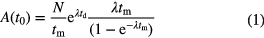
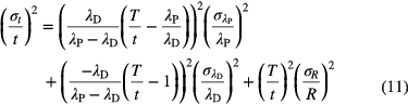
The counting factor, 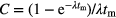 , accounts for decay during the measurement and is significant (>x%) only if tm is not negligibly small compared to the half-life T1/2 = ln2/λ or, using a first order series expansion
  if
if 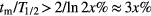 .
.
The standard uncertainty of the half-life,  , propagates through the decay correction factors as follows
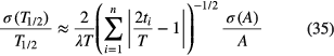
The uncertainty on the corrected activity increases linearly in time (via td and tm, if tm < T1/2) and the propagation factor is significant for time periods of comparable magnitude as the half-life. With every 0.1% uncertainty on the half-life, the uncertainty of the activity increases by 0.07% per half-life.
Routine laboratories calibrate their activity detectors by means of secondary standards; calibrated sources with traceable activities of certain radionuclides. These standards are kept and reused for a practical period of time. Consider for example 10 year-old 22Na (2.6029 (8) a), 54Mn (312.13 (3) d), 55Fe (2.747 (8) a), 57Co (271.80 (5) d), 65Zn (244.01 (9) d), 109Cd (461.4 (12) d), 124Sb (60.208 (11) d) and 134Cs (2.0644 (14) a [21]) sources being used for calibration in an x- and γ -ray spectrometry laboratory. The standard uncertainty on the calibration factor due to uncertainty on the half-life is then respectively 0.08% (22Na), 0.08% (54Mn), 0.7% (55Fe), 0.17% (57Co), 0.4% (65Zn), 1.4% (109Cd), 0.8% (124Sb) and 0.23% (134Cs), which is significant for some of these nuclides. Larger errors can occur for radionuclides with shorter or less reliably known half-life.
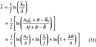
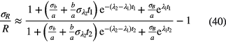
More intricate rescaling is applied in the field of neutron activation analysis, where the link between elemental concentrations and measured activity of decay products is established through complex activation and decay formulas obtained as solutions of sets of linear first-order differential equations [22]. They typically contain a saturation factor  for the activation during a period tirr, a decay factor
  and a counting factor C as above. The relative uncertainty of a measured count rate via such factors SDC is
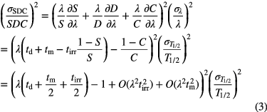
Assuming that the time periods involved—tirr, td and tm—are of similar magnitude, the propagation factor is about 1 for long-lived nuclides (λt << 1, λtirr(1 − S)/S ≈ 1, C ≈ 1) and λtd + 1 for extremely short-lived nuclides (λt >> 1, λtirr(1 − S)/S ≈ 0, λtm − (1 − C)/C ≈ 1). For intermediate half-lives (λt ≈ 0.1–1), the propagation factor can be <1 or even cancel out completely, because the activation and decay terms have opposite signs.
2.2. Radiometric dating
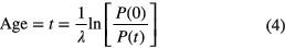
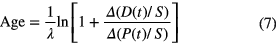
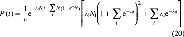
Radiometric dating methods are based on the exponential decay law describing the decreasing number of radioactive atoms in a material, and/or the related ingrowth of daughter nuclides [23]. One way of age dating is based on known atomic concentrations P(t) of the parent nuclide at different times, via
A typical example is 14C dating (5700 (30) a).
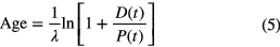
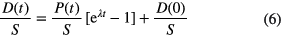
If the daughter atoms are stable and their initial concentration is zero, D(0) = 0, the sum of parent and daughter concentrations is constant, D(t) = P(0) − P(t) or P(0) = P(t) + D(t), and the age can be obtained from
This scheme can be used in uranium-lead dating for systems that remained closed and with both decay routes 238U/206Pb and 235U/207Pb yielding concordant ages.
Corrections are required if D(0) ≠ 0 or if the concentrations have varied in the sample through physicochemical processes. Isochron dating methods use the concentration S of a stable isotope of the daughter element as a reference. Since (P(0) + D(0))/S = (P(t) + D(t))/S, the relative concentration of the daughter isotopes D(t)/S is the sum of the initial isotopic ratio D(0)/S and a fraction originating from the decay of the parent nuclide:
As P(t)/S can vary freely within material samples of the same age, a consistent set of data is characterised by a linear relationship, called isochron. The age follows from the slope (eλt − 1)
This procedure is routinely used in rubidium-strontium dating, in which the parent 87Rb and daughter 87Sr are compared to stable 86Sr. Ratios are used instead of absolute concentrations because they are conveniently measured with mass spectrometers. Another application is dating 'young' groundwater, i.e. assessing when it became isolated from the atmosphere, through the decay of tritium 3H to the rare stable daughter 3He.
The isochron method can also be applied in uranium-lead dating, using 204Pb as the non-radiogenic isotope. Combining the isochron equations for the 238U/206Pb and 235U/207Pb systems, one can derive the mathematical basis of 'lead-lead dating' based merely on measurement of the lead isotopic ratios R6,4(t) = 206Pb/204Pb and R7,4(t) = 207Pb/204Pb
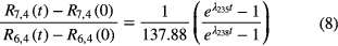
where the factor of 137.88 is the present-day 238U/235U ratio. The initial Pb isotopic ratios (extracted from meteorites) and age of the system are the two factors determining the present day Pb isotopic ratios. In a closed system, equation (7) represents a linear relationship in which the slope depends on the age. The age of Earth, 4.54 (5) 109 a, was thus obtained (see e.g. [24]).
The dating equations (4), (5) and (7) are linearly proportional to the half-life of the parent (and equation (8) roughly on a ratio of half-lives), which means that the relative uncertainty of the half-life constitutes an upper limit to the attainable accuracy on the age. For several applications, this has become the bottleneck [25].
Another dating technique, 210Pb sediment radiochronology [26], is frequently applied to reconstruct past environmental conditions of ecosystems. In systems that have been closed for a sufficiently long time (>150 a), the supported210Pb is in equilibrium with its parent radionuclide 226Ra. Due to various transport processes, e.g. exhalation of 222Rn and subsequent deposition of daughter products, excess or unsupported210Pb can accumulate in bottom sediments. The amount of excess 210Pb in various layers of a sediment core is an indicator of the accumulation rate. For this technique, the uncertainty on the half-life is of minor importance compared to the modelling issues and the measurement uncertainty on the difference between 210Pb and 226Ra/214Pb activities.
2.3. Nuclear forensics
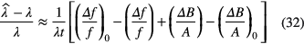
Radioactive disequilibrium between parent and daughter arises when both are separated by physicochemical processes, e.g. by applying radiochemical separation techniques. Following this separation, the daughter starts to grow in again. Information on the time of separation may be obtained from measuring the ratio of parent to daughter atoms. This property is applied in nuclear forensics, aiming at fingerprinting of nuclear materials [23, 27, 28]. The relative amounts of parent and decay products can be used to identify the age and source of the material. Nuclides of interest are actinides (Th, U, Np, Pu, Am) with potential applications in improvised nuclear devices or other nuclides that can be applied in radiological dispersion devices (Co, Sr, Cs). A sample consisting of mixed U-Pu isotopes provides as many as a dozen chronometers, including 234U/230Th, 235U/231Pa, 238Pu/234U, 239Pu/235U, 240Pu/236U and 241Pu/241Am. The time scale of interest is in the 1–50 year range, which is much shorter than in geology. Age dating of U is more difficult than Pu dating, because their long half-lives lead to minute amounts of ingrowing daughter nuclides. Besides the quality of the separation, the current uncertainties on the relevant half-lives are a major limiting factor on the attainable accuracy.
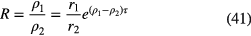
Parent and daughter both being unstable, the ratio of their atom concentrations at a time t after complete separation (D(0) = 0) is calculated from [29]
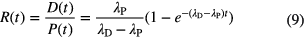
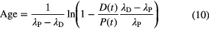
and the 'age' t is solved from
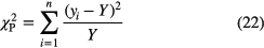
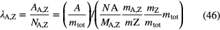
Linear propagation of uncertainty on the atom ratio R(t) and the half-lives λP and λD results to [29]
in which the variable T is defined through
For material with a relatively young age compared to the half-lives involved, λPt << 1 and λDt << 1, the propagation factors for λP and R are unity, while the factor for λD is insignificantly small. Consequently, age determinations based on atom ratios are more sensitive to the parent half-life than to the daughter half-life. This is compatible with the fact that R(t) ≈ λPt for small values of t, i.e. linear with λP and independent of λD.
Only for old material, |λD − λP|t >> 1, does the uncertainty propagation of the daughter half-life become important, but under these conditions, the over-all accuracy of the method is relatively poor as the propagation factors increase almost exponentially with λDt.
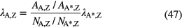
Similar equations can be derived for cases in which the activity ratio RA of parent and daughter nuclide is measured instead of the atom ratio, with a subtle change in a multiplication factor
The uncertainty propagation of the concentration ratio RA(t) and the half-lives λP and λD to the age is given by [29]
For material with a young age compared to the half-lives involved, λPt << 1 and λDt << 1, the propagation factors for λD and RA are unity, while the factor for λP is insignificantly small. Consequently, age determinations based on activity ratios are more sensitive to the daughter half-life than to the parent half-life, which is the opposite of the effect noticed for atom ratios (equation (11)).
Activity ratio measurements enhance the signal of the short-lived nuclide, and may be a good alternative to atom ratio measurements in cases where the atom concentration of the short-lived nuclide is particularly low. The relative uncertainty of the half-lives of the parent (via R) or the daughter nuclide (via RA) is of equal importance as the relative uncertainty of the measured ratio (R or RA). In order to achieve a time resolution of 50 d (k = 1) over a period of 1–50 years, the half-life uncertainties need to be lower than 0.25%, which has not yet been achieved for several important nuclides.
2.4. Dating of a nuclear event
The principles of radiometric dating can also be applied to fission products created in a nuclear explosion. Radionuclides may attach to aerosols or be released as noble gases and get collected in air samplers at a remote location. One can distinguish isobaric and non-isobaric clocks [30]. Non-isobaric clocks start from theoretical (cumulative) fission yields for the calculation of initial activity ratios and use the current activity ratio of fission products with different half-lives to estimate the time elapsed since the nuclear event. Isobaric clocks are based on parent–daughter pairs of which the daughter nuclide is not directly produced in the fission reaction. The equations are the same as the equations (9)–(14) applied in nuclear forensics. For example, they are directly applicable to the 140Ba-140La clock [31], based on progeny of the short-lived noble gas 140Xe (13.6 s). The aerosol-bound 95Zr-95Nb chronometer is another important clock that requires a more elaborate mathematical treatment due the presence of meta-stable 95mNb in the decay scheme [32]. Specific equations for time-zero and uncertainty calculation are available to perform bias-free 95Zr-95Nb dating of a nuclear event over a time range of more than a year [33].
2.5. Nuclear medicine
Radionuclides introduced as nuclear medicine into the human body deliver a dose that depends on their effective half-life Teff = ln2/λeff, a combination of radioactive decay and biological excretion:

Starting from an initial activity A, the accumulated dose is proportional to the number of atoms that decay in the body:

The relative uncertainty of the effective half-life propagates linearly to the dose. The biological half-life cannot be determined as precisely as the physical half-life, and the dominance of either rate differs from one radionuclide to another. For many long-lived nuclides, such as 3H, 14C, 22Na, 36Cl, 60Co, 137Cs and 235U, the much shorter biological half-life (10–70 d) is dominant [34]. The inverse is true for short-lived nuclides, such as 32P, 59Fe, 99mTc, 123,131I, 140Ba and 198Au. The latter are the only cases in which the dose calculation depends significantly on the accuracy of the physical half-life. The bone seekers 90Sr, 226Ra and 239Pu have extremely long effective half-lives (18–197 a [34]), which reduces their uncertainty propagation towards the accumulated dose during a person's lifetime.
3. Measurement of short half-lives
Half-lives of excited nuclear states, giving access to transition probabilities, provide direct insight into the structure of the nucleus and offer one of the most stringent tests of nuclear models. Different measurement techniques are applied to cover half-life ranges between picoseconds and seconds.
3.1. Picoseconds–nanoseconds
Short lifetimes of excited nuclear levels ranging between about 1 ps to several ns have been measured by the Recoil Distance Doppler-Shift (RDDS) method [35, 36] for a large variety of nuclei all over the nuclear chart. In this method, nuclei produced by a beam-induced nuclear reaction in a thin target are allowed to fly freely in vacuum over variable distances from the target to a stopper ('plunger'). Gamma-spectroscopy measurements are performed with a single off-axis HPGe detector, preferably at extreme forward or backward angles, or by a cluster of detectors arranged at the same polar angle to increase sensitivity. Gamma rays emitted in flight are distinguished from those emitted after the nucleus has come to rest in the stopper, due to their Doppler shift. The mean life of a given level (and the accumulated time delay from higher lying states that feed it) can be deduced from the relative intensities of the shifted and unshifted peaks at different target-to-stopper distances.
In principle all the effects which should be considered when applying the RDDS method were known right from the beginning when the method was developed, but from time to time some of these effects were underestimated or invalid assumptions were made. In some cases the reasons for failures could be identified later but for other cases the situation remained unclear. Typical sources of uncertainty mentioned in the review paper by Dewald et al [35] are:
- fit of decay curve: the decay curve comprises of a single exponential if only one excited level is involved, but usually a more complex level-feeding scheme needs to be solved with many free parameters, such as level lifetimes, branching ratios and initial populations. Assumptions have to be made for time behaviour of side-feeding, i.e. level feeding for which no discrete transitions are observed. Advanced code was developed to deal with the complexity of the non-linear fitting problem, but in many cases the solution is not unique. In general, the function to be fitted is not exactly known since the feeding states are not completely known.
- distances and solid angles: the standard method relies on absolute distances, incl. the position of the plunger. Solid angle effects show up in the shifted peak when the target–stopper distance becomes comparable to the stopper–detector distance. In this case, only the unshifted component is analysed or a fixed stopper and moving target is used instead.
- detector efficiencies: the shifted and unshifted peaks are registered with different detector efficiencies, depending also on the angle of observation with respect to the recoil velocity.
- relativistic effects: high recoil velocities affect the lifetime of the excited nuclear state (time dilation), the emission angle (aberration) and the solid angle (Lorentz boost).
- line shapes: knowledge of the line shapes of the shifted and unshifted peaks is needed when both are not well separated. The recoil velocity distribution is significantly broadened and asymmetric due to the finite target thickness. Moreover, the faster recoils reach the stopper in a shorter time and therefore contribute less to the area of the flight peak. Also during slowing-down time in the stopper, the ion velocity changes magnitude and direction, leading to a tailed γ-line shape that prevents determination of comparably small lifetimes.
- deorientation: the angular distribution of the γ-ray emissions becomes more and more isotropic with increasing flight time, due to a decay of the spin orientation during the relaxation period. Even though this effect has been known for a long time, it was often underestimated, resulting in wrong half-lives. The error may reach 20% when using only the unshifted peak or 6% when using both.
These problems stimulated efforts to improve the technique with respect to higher reliability and to make it more transparent so that the presence of possible systematic errors is revealed more easily. Some of these improvements are [35, 36]:
- γ–γ coincidence measurements: by gating on specific feeding transitions, the problem of side-feeding and unknown feeding intensities and times can be circumvented. The drawback is the need for longer beam time and many Ge-detectors. Gating as a means of reducing background is beneficial to the statistical precision only if it improves the peak-to-background ratio by a large factor.
- the differential decay curve method and new alternatives: powerful new analysis techniques help solve problems of the standard method, relying more on experimentally accessible data, requiring only relative flight times/target-to-stopper distances and taking into account the angular and velocity spread of recoiling nuclei due to energy loss and multiple scattering in the target.
3.2. Nanoseconds–microseconds
Nano- and microsecond nuclear states are mostly measured electronically in delayed coincidence experiments or alternatively by time interval analysis.
3.2.1. Delayed coincidence counting.
The radiation yielding the state of interest is detected to provide a start pulse for an electronic clock, and the radiation by which the state decays is detected in the same or another device to provide a stop pulse. The half-life is derived from the analysis of the time difference between both signals. Using ultrafast scintillators (plastic scintillator, LaBr3(Ce), BaF2), the applicability range of the method has been extended down to picoseconds [37]. Also states of tens of milliseconds (or even seconds) are within reach, provided that the count rate is sufficiently low. Conventional experimental set-ups contain electronic modules, such as delay line amplifiers, timing single channel analysers (TSCA), time-to-amplitude converters (TAC) and multi-channel analysers (ADC), but they can also be replaced by programmable processors (FPGA) or software performing off-line data analysis of digitally acquired data saved in list files [38].
Common features of the delayed coincidence method are that time differences are stored in a spectrum, that the decay constant is derived from the slope of an exponential function fitted to a part of the spectrum and that account has to be taken for data not due to the intended parent–daughter pairs. Random coincidences may be recorded due to background signals, decays from other states or closely spaced but unrelated parent and daughter events. The first two interferences can be significantly reduced if the experiment allows for energy selectivity, e.g. by selecting peaks in γ- or α-spectra, and the third by keeping the count rate well below the decay constant. By means of energy selection, multiple half-lives can be derived from one experiment.
There exist different variants of how the data are recorded, each requiring a specific mathematical basis for the functional shape of the time spectrum. Two options are discussed below, based on different manners to collect and interpret time differences.
- Single delayed coincidence
In a classical set-up, a timer is started whenever a parent decay is detected and stopped when a daughter decay is detected. Then the system is made sensitive again for parent decays. In doing so, all the parent events arriving before the first daughter event are ignored. In this type of experiment, the time spectrum theoretically takes the following shape: [39]

in which A and B are multiplication factors related to efficiency and count rate, λ is the decay constant of the state of interest and R2 is the count rate of the daughter decay. If the count rate R2 is kept small (R2 << λ), this formula can be approximated by:

which is commonly used for the determination of a half-life from experimental data.
- Multiple delayed coincidences
If the activity of the source is high − i.e. R2 is not negligible compared to λ − the true parent–daughter decays are being interfered by uncorrelated events, leading to a distortion of the single-coincidence time spectrum. In that case, systematic errors are to be expected from using equation (18). This can be solved by means of an alternative time analysing circuit in which a parent decay starts the timer and not a single but multiple delayed coincidences are added to the time spectrum, one time value for every recorded daughter decay over a long period of time [40]. Theoretical analysis [39] predicts that time spectra obtained by this approach are represented by the sum of a constant term and an exponential function with the time constant of the radioactive decay of the daughter, exactly as in equation (18). Using multiple delayed coincidences eliminates the spectral distortion effect, but at the price of an increased number of random coincidences.
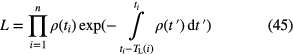
3.2.2. Time-interval distribution analysis method.
Time-interval distribution analysis is a well-established method for measuring the activity of radiation sources [41–43]. For a simple decay, the probability density of the time interval between two successive disintegrations is given by the formula:

in which λN denotes the activity of the source. This formula can also be applied to a good approximation in short time intervals for a mixture of long-lived radionuclides − decaying independently or in radioactive equilibrium in a decay chain − but is incorrect if the decay chain also contains short-lived members. Lindeman and Rosen [42] deduced the general formula for the time-interval distribution of decays from a long-lived parent in equilibrium with n − 1 short-lived daughters. For a large number of parent atoms N1, the probability of a given time interval between two successive disintegrations is given by:
It shows that, at low time intervals, the shape of the curve has a term that depends not on the activity of the daughter nuclide, but on its half-life. The time-interval spectrum is obtained by binning the time differences between all events. It is possible to focus on one of the transitions separately by selecting regions in the energy spectrum mainly belonging to the parent-daughter sequence of interest. The resulting curves have the characteristics of equation (20) applied to a single daughter nuclide (i = 2), but need the inclusion of a weighting factor C to balance both parts of the curve:

in which C is included as a free parameter in the fit. For a source in equilibrium, the number of short-lived daughter atoms N2 = N1 λ1/λ2 will be low compared to N1 and thus the second term in the first exponential is small. Time-interval distribution analysis yields comparable results to the delayed coincidence method [38, 43].
3.2.3. Data analysis.
The half-life of the nuclide is usually derived from a least-squares fit of an exponential function to the measured time spectra. However, some complications have to be taken into account. Least squares fitting procedures imply the assignment of proper weighting factors to the stochastically distributed data involved. In the case of a Poisson distribution, the obvious choice of setting the weighting factor equal to the inverse of the measured value is prone to bias towards low values. Alternatively, using the inverse of the fitted value may turn out to be biased towards higher values, depending on the procedure followed. Additional problems arise when also the possibility of zero counts has to be taken into account. An overview of the problems and possible solutions can be found in [44, 45] and references therein.
In fact, it is possible to perform unbiased least-squares fitting with Pearson's chi-square i.e. using the fitted value Y as weighting factor,
on condition that the weighting factor is kept fixed during each iteration of the fit. After each optimisation, it is set equal to the fit value Y obtained in the last iteration and a new fit is performed until convergence is reached [45]. There exist alternative estimators that allow using existing software for least-squares in a less biased way, with a minimal adaptation to the procedure. For example, one can minimise [45]
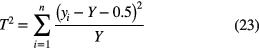
freely without the need for an iterative procedure, and obtain an unbiased result if the data are not too close to zero.
A recommended solution to the problem of bias is to replace the χ2 estimator by a maximum likelihood ratio statistic (MLE) for Poisson distributions [44]:
in which yi is the observed number of events in time bin i, Y is the fitted value and the last term is set equal to zero for yi = 0.
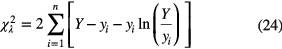
To decay curves with a (quasi) purely exponential shape, another excellent method to derive an unbiased value for the decay constant is applying 'moment analysis'. It is known that the 'first moment' (i.e. the expectation value for the decay time t) and the 'second central moment' of the exponential distribution are equal to λ−1 and λ−2, respectively. If the moment analysis of the decay curve is restricted to a time interval (t1,t2), the following relationship can be derived between the half-life and the first moment [45]:

and with the second central moment [45]:

in which the correction factors Ci are calculated from:
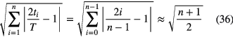
The statistical uncertainty associated with equation (25) is:
in which  represents the number of events observed within the time interval (t1,t2). The relative uncertainty associated with T1/2 of equation (26) is about a factor √2 higher, i.e. proportional to
  . Equation (26) confirms the observation by others [46, 47] that the best attainable precision on a decay constant is equal to 1/√N.
The first moment, which is not a central moment, is sensitive to the time value assigned to each time bin. The data being distributed into time bins of equal duration Δt, the weighted mean time value of the first time bin, going from t = 0 to Δt, is calculated from:
The time values for the other bins are found by adding to equation (29) a multiple of Δt. Central moments are insensitive to a linear translation of the time origin. Moment analysis should be performed only in a region (t1,t2) of the spectrum in which the random coincidence part (B in equation (18)) or contributions of other nuclides with a significantly shorter or longer half-life are negligible.
3.2.4. Uncertainties.
The time spectrum is the convolution of the prompt peak (the width of which shows the variation in the timing between truly coincident events) and the slope generated by the lifetime of the nuclear level. For relatively long half-lives, the width of the prompt peak is negligibly small and the half-life is extracted from a fit to the exponential slope. If the half-life is short compared to the time resolution of the detection system, the time spectrum resembles the prompt peak of which the centroid has been displaced. The lifetime can be extracted from this shift [37]. The 'shift' method is less precise than the 'slope' method.
Typical uncertainty components are:
- time resolution: indicates the lowest time difference that a coincidence set-up is able to determine. It is represented by the FWHM of the prompt time spectrum, which is generally a Gaussian distribution obtained by measuring simultaneous events in the two timing branches. Contributors to the FWHM are variances due to scintillator, photomultiplier and time pickoff.
- Time jitter in a scintillator is proportional to the figure of merit
 , in which τf and Nf are the intrinsic decay time and light yield of the scintillator, respectively. Photomultipliers are matched to the scintillator for maximum spectral response at the required wave length, large quantum efficiency, short rise time, transit time and transit-time spread. The development of ultrafast scintillators and multipliers have contributed most to improving the sensitivity of the fast timing technique down to the picosecond region.
 - walk, drift: whereas jitter is caused by noise and statistical fluctuations of the signals, walk stems from differences in pulse shape and amplitude and drift relates to aging and temperature variations. These effects are considerably reduced by using constant fraction discrimination, resulting in a bipolar pulse of which the zero crossing is nearly independent of pulse height. This results in more precise time pickoff.
- counting statistics: statistical precision lowers the uncertainty on either the centroid shift or the slope of the time distribution. Ideally the best attainable precision is 1/√N.
- secondary effects: systematic errors due to difference in the traveling time of particles and photons from source to detector as well as spatial distribution of interactions within the detector, ambiguity in the separation of parent and daughter radiation, scattering of radiation between detectors, spurious shifts due to changing counting rates, time calibration and its linearity, different signal velocities in cables, interfering signals from other transitions, etc.
- data analysis: the theoretical model of the time distribution analysis has to match with the electronic scheme by which the data were collected. Parent-daughter transitions should be correctly separated from random coincidences and interfering signals, while influences from the latter need to be accounted for in the uncertainty. For example, one can quantify the sensitivity of the decay constant to an error on B in equation (18) by fitting a hypothetical λ for B ± σ(B). In spectra with low counting statistics and long slopes, the least-squares analysis underestimates the lifetime and proper fitting should be based on Poisson statistics [37].

4. Measurement of intermediate half-lives
4.1. Decay curve
Many radionuclides with practical implications and applications have half-lives varying between seconds and about 100 years. This is a range of half-lives that can be measured directly by repeated activity measurements of a source. The simplicity of the measurement principle has incited many authors to publish thus obtained half-life data, unsuspecting of hidden processes that inflate the measurement errors far beyond their uncertainty estimates. A common scenario is that an exponential decay curve is fitted to various activity values measured as a function of time and that the uncertainty on the decay constant is obtained from the least-squares minimisation algorithm. This procedure is often faulty [48], as real measurement data may deviate in a subtle but systematic way from the theoretically assumed decay curve. The fitted decay constant is the value leading to the smallest residuals, which explains why an erroneous result seldom raises suspicion in the mind of the experimenter [14, 15]. Also other methods can be applied to extract the half-life from the data, such as moment analysis (section 3.2.3) and statistical sampling [14, 49], but they are equally sensitive to systematic errors.
The sum of an exponential function superposed on a constant background is often assumed to model the temporal dependence of the measured activity:

The fitted value of the parameter λ is believed to be the most probably value of the decay constant and the uncertainty is derived from the covariance matrix provided by the fitting algorithm, which implicitly assumes that the measurement data rigorously follow the prescribed decay function, the residuals being purely stochastic. In reality, there is a less than perfectly linear relationship between the activity and the measured signal (count rate or current) in a detector. Various processes make measurement data deviate from the ideal decay curve, long-term instabilities being at the same time the most influential but least visible sources of error. Due to differences in uncertainty propagation, it is convenient to subdivide these process according to the frequency at which they occur [14, 15]:
- High-frequency deviations: these sources of uncertainties occur at a rate that is higher than or comparable to the measurement duration of one data point. A typical example would be counting statistics: Poisson processes are characterised by an exponential distribution of the interval times between successive events. By extending the measurement, one improves the statistical uncertainty on the actual count rate. Also ultra-high frequency instabilities, such as e.g. electronic noise, are included in this category. They are partly cancelled, though, by the 'integrating' effect of the duration of the measurement. Normal statistical treatments (including least squares fitting) apply because of the preservation of randomness of the data.
- Medium-frequency deviations: these instabilities show up (at least partly) as a trend in the residuals and can also be identified by means of an autocorrelation plot [14]. They include the so-called 'seasonal effects' (e.g. day-night effects or changes with the seasons of the year), but also other variations occurring at a rate that can be observed over the measurement campaign. Their effect on the fitted half-life is greatly underestimated if treated as just a random residual. Moreover, a fit tends to minimise the residuals and partly covers up the true size of the medium frequency effects. Typical examples are the activity interference by radioactive impurities, reproducibility of the source-detector geometry, noticeable changes in the detector efficiency (e.g. through temperature, pressure, humidity, electronic flaws, scale changes in an electrometer) and modelling errors (e.g. neglecting a decay correction during measurement when progressively adjusting the measurement duration with time, inadequate separation between photopeak and underlying Compton continuum by gamma-ray spectrometry).
- Low-frequency deviations: these sources of uncertainties occur at a rate that is lower than or comparable to the duration of the whole measurement campaign. They remain practically invisible in the residuals, as the fit will compensate for this trend, hence erase it erroneously. Common problems in this range are a non-linear detector response to activity (charge recombination in ionisation chamber, discharge of a capacitor, non-linearity in an electrometer, pile-up and dead time in counter), systematic errors in the background subtraction, under- or over-compensation of count loss by live-time systems (double count loss through summing-out of piled-up events, hidden dead time due to unexpected behaviour of detector and electronic modules, pulse undershoot and overshoot, cascade effects of pile-up and dead time, effect of variation of dead time during measurement of short-lived nuclides), long-term drift of the counting efficiency and source degradation (e.g. oxidation of the source, mechanical wear, precipitation of active material in a solution).
In figure 1, hypothetical residuals of a fitted decay curve to data with high, medium and low frequency instabilities are shown. The dark dots represent the deviations of the data from the 'true' decay curve, the light circles show the deviations of the data from the fitted decay curve and the solid curve is the difference between the fitted and true decay curve. The observer that performs the fit perceives only the light points. Considering that a slope equal to zero corresponds to the true half-life, the medium and low frequency deviations in figure 1 lead to a biased result. As the residuals give insufficient indication of these errors, one has to evaluate an exhaustive list of potential uncertainty components and combine them in a squared sum in the uncertainty budget.

Figure 1. True (dark dots) and perceived (light dots) residuals from a fit of a decay curve through hypothetical data affected by high (top), medium (middle) and low (bottom) frequency instabilities. Systematic deviations are not fully observed by the experimentalist, as the fit tends to minimise them.
Download figure:
Standard image High-resolution image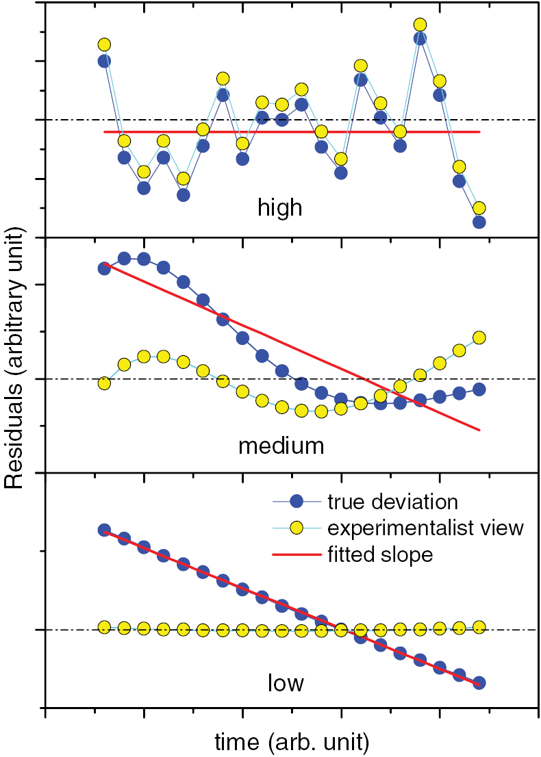
4.2. Impact of systematic errors
In a simplified scheme, the decay constant in equation (30) can be determined from two activity measurements of a source: A0 at t = 0 and A at time t. Generally, corrections have to be made to transform the measured signals  into the activity A of the radionuclide, which can be represented by a subtraction of a value B (e.g. background signals) and multiplication by a factor f (e.g. dead-time correction). The estimated value of the decay constant is
Errors ΔB and Δf in the corrections propagate into an error in the decay constant:
Some conclusions can be derived from equation (32):
- Assuming the errors to be constant, the uncertainty on the half-life is inversely proportional with time via the factor 1/λt. Consequently, in order to reduce the uncertainty by a factor of two, one needs to double the decay time. This entails a linear relationship on a log-log scale, therefore less and less is gained by continuing the experiment at great length. Moreover, the gain in accuracy can be counteracted by a long-term increase of ΔB/A and Δf/f with time.
- A systematic relative error Δf/f = (Δf/f)0 does not alter the half-life result; e.g. there is no need to determine the detection efficiency of the detector, as long as it is constant in time. On the other hand, a systematic error in the characteristic dead time leads to non-constant relative error in the count-loss correction factor. Some authors, even in recent publications, make the error of emphasising efficiency calibration over linearity checks.
- The impact of systematic errors ΔB in background (or impurity) subtraction are dependent on their size relative to the net signal A. Energy-selectivity is a useful tool to separate the source activity from interfering signals and to be insensitive to variations in threshold settings and instrumental noise. Therefore it is easier to measure half-lives through (high-energy) gamma rays and alpha particles than through (low-energy) x-ray, electron and beta emissions. The latter decay types are more sensitive to medium-frequency instabilities, which explains the speculations about the non-constancy of half-lives involved in, e.g. electron capture decay.
- The ideal time interval for a measurement campaign is typically chosen in function of non-linearity effects at the start (e.g. dead-time, short-lived impurities) and poor signal quality at the end (e.g. counting statistics, background subtraction, long-lived impurities, instability).
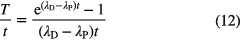
4.3. Uncertainty propagation
The uncertainty propagation formula for a half-life T1/2 = T ln2/lnR determined from the activity ratio R = A/A0 at time t = 0 and t = T is
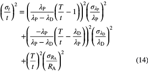
In practice, measurements are repeated at regular time intervals during a measurement campaign over a time interval [0,T], with the intention to reduce the uncertainty on the half-life. Assuming a hypothetical situation in which the relative uncertainty on the activity measurement σ(A)/A is identical for each data point, the uncertainty propagation can be calculated from [50]:
The formula implicitly assumes that the data are independent; therefore, it is applicable only to statistical (short-term) variations and not to auto-correlated (medium and long-term) variations. When performing three measurements, the middle data point neither affects the half-life nor its uncertainty. It makes a fitted decay curve shift as a whole in the vertical direction, but does not alter its slope.
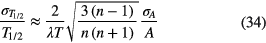
A similar approximating formula was derived independently [14, 15] from the assumption that the relative impact of a measurement on the fitted half-life is proportional to the time difference with the middle of the campaign, i.e. ~│t − T/2│/(T/2). Under the aforementioned conditions, and data points being spread somewhat evenly in time over the period T, the uncertainty on T1/2 is approximated by:
and the reduction factor (for n > 2) is roughly equal to
resulting in
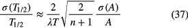
Using equations (34) or (37), an evaluator as well as an experimenter can make a quick estimate of the contribution of, e.g. counting statistics to the half-life if three variables are available: the number of activity measurements, n, the duration of the campaign, T, and a measure of the uncertainty for a typical activity measurement, σ(A). Equation (34) is probably more rigorous for large n, but the difference is less than 20% and significant only in the rare case that high-frequency uncertainty components are dominant. If an uncertainty component σ(A)/A is not constant with time, an average is taken of its value at time t = 0 and t = T.
It is important to apply independent uncertainty propagation according to the 'frequency' of the uncertainty components. When pertaining to medium and low-frequency instabilities, the parameter n in equations (34) and (37) receives a new meaning. For (cyclic) medium-frequency components, the value of n is set equal to the number of periods covered by the measurement campaign. In the case of, e.g. yearly repeating effects, n would correspond to the number of years covered. For low-frequency effects, the value n = 1 is always selected and the propagation factor is 2/λT. For example, a hypothetical 1% change in detection efficiency during the measurement campaign leads to an average uncertainty at t = 0 and t = T of < σ(A)/A > = (0% + 1%)/2 = 0.5% and is propagated to an uncertainty of σ(T1/2)/T1/2 = 1%/ λT, in agreement with equation (33).
Whereas two activity measurements in principle suffice for a half-life determination, repeated measurements have the advantage of reducing the propagation of random uncertainties, as well as allowing quantification of medium frequency components if they are not insignificant compared to the random variations. For this purpose, it is important to measure with good statistical precision. As time progresses, the main weight of the uncertainty budget typically shifts from random variations to cyclic instabilities and systematic errors [14]. The latter are the most difficult to quantify, so the most precise half-lives have the most uncertain confidence intervals. Also the analysis method itself may contribute to unexpected errors, as already discussed in section 3.2.3.
4.4. Examples
4.4.1. Reproducibility in ionisation chamber (IC).
Ionisation chambers are well-suited for half-life measurements because of their stability over decades, in particular if that stability is regularly monitored with a long-lived check source. Often a 226Ra source is used for that purpose, which requires care that its radon daughter is well-contained; 166mHo is considered an interesting alternative. Instability may occur if, e.g. the chamber leaks gas, the background rate varies due to external sources, radon emanation discharges an air capacitor, the charge collection or current measurement devices are replaced or their capacitance is adapted to the activity range. For this reason, current measurements of mononuclidic sources are often performed relative to the reference source.
In spite of using the aforementioned method, there appeared to be a mysterious inconsistency between a suite of half-lives obtained at PTB [51] and NIST [52]. While the decay curves of, e.g. 60Co, 133Ba, 137Cs, 152Eu and 207Bi obtained in both laboratories looked exponential, they had different slopes. The explanation was eventually found in a gradual slippage of the positioning ring that determines the height of the sample in the re-entrant tube of the NIST ionisation chamber during 35 years of use [53, 54]. This unaccounted-for height change caused a change in the detector response on the order of 10−5 to 10−3 per year, depending on the radionuclide. The changes are dependent on γ-ray energy and have particularly affected the half-lives of long-lived nuclides with different IC response than the reference source. The long-term instabilities remained unperceived in the residuals of the fitted decay curves, yet simulations of their influence have led to significant corrections (~1%) and an increase of the uncertainty [53, 54].
4.4.2. Impurity and background correction.
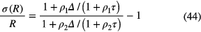
An ionisation chamber is used to measure a source that is not perfectly mono-nuclidic due to the presence of an impurity, possibly a radionuclide occurring in the same decay chain. Gamma-ray spectrometry may be used to determine the relative activity of both nuclides and to calculate the impurity signal in the IC to be subtracted. Errors in the γ-ray emission probabilities and response of the IC and spectrometer can influence the half-life result. As an alternative, the signals of both nuclides can be fitted simultaneously to the decay curve. Another possible source of error is neglecting the decay rate change during measurements of variable duration, which requires a different correction factor  (see also section 2.1) for the fractions of the signal associated with both decay constants. The following function can be fitted to the measured data (average current over a measurement time interval [55]):

in which a and b are constants and B represents the background signal. For measurements of constant duration tm in real time, the factors Ci are invariable and can be integrated in the factors a and b. Assuming that these corrections have been taken into account, the activity ratio at two different moments in time t = t1 and t = t2 is calculated from:
in which I(t) is measured IC current,  is a fitted or calculated impurity signal and
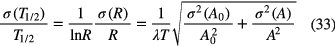
  is the measured or fitted background signal. The most straightforward way to investigate the uncertainty on the half-life T1/2 = (t2 − t1)ln2/lnR due to potential errors on background and impurity subtraction is to compare the result of hypothetical half-life calculations using equation (38) with different values of
  ,
,  and
and  . Alternatively, one can calculate the uncertainty from a first order series expansion [55] and equation (33):
The fitted values of background  and impurity signal
  may be anti-correlated as they compete in describing the part of the decay curve not following the exponential decay of the main nuclide. This should be taken into account when combining the different uncertainty components. It is important to take into account that the number of background counts may show statistical fluctuations higher than expected from a Poisson process. It is good practice to include a fraction of
  also as a hypothetical systematic uncertainty component, e.g. because the counting conditions for a blank and a source may differ.
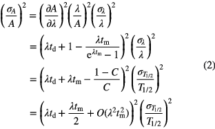
The above reasoning and equations (38)–(40) are also formally applicable to the case of a parent and daughter half-life being derived simultaneously from a fit to an ingrowth-and-decay curve obtained with an IC or calorimeter. The resulting half-lives can be highly correlated and their uncertainty underestimated. For example, this could be the case with 227Th where applying a fixed value for the half-life of the 223Ra daughter has led to a significant but questionable reduction of the uncertainty estimate (see discussion in [56]).
4.4.3. Counting with dead time and pileup.
The activity is registered as a pulse counting process, as opposed to current measurements in non-selective methods as ionisation chambers and calorimeters. The weakness of counting methods lies in the finite time resolution of the detector and associated pulse processing electronics [57, 58]. The linearity of the detector response is affected by count loss due to pulse pileup and system dead time. This prohibits the use of high amounts of activity at the start and therefore shortens the duration of the measurement campaign, since it is also limited at the end by poor counting statistics and significant background subtraction.
Live-timing techniques can compensate for count loss, by accounting for the characteristic dead time τ associated with each recorded event. If the dead time is of the extending type, the activity ratio R of the activities A1 and A2 at a time t1 and t2, respectively, is obtained from the measured count rates r1 and r2 and an exponential correction factor [57–59] to estimate the true input rates ρ1 and ρ2:
The relative error on R produced by applying a slightly incorrect characteristic dead time τ + Δ is
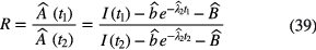
in which TR and TL represent the system real time and live time, respectively, and the ratio of both corresponds to the dead time correction factor used in the respective measurements. The error grows exponentially with the count rate ρ1, which overrules the 1/λT reduction factor in the uncertainty propagation to T1/2 (via equation (33)):
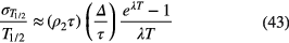
For a fixed end point of the measurement campaign with count rate ρ2, the uncertainty due to extending dead time or pileup increases by a factor of 1.5 or more for every half-life that the measurement campaign is started earlier. Therefore, there is no gain in accuracy by increasing the initial activity if dead time or pileup is the main uncertainty component.
In the case of non-extending dead time, the uncertainty on the activity ratio is
and propagates to T1/2 via equation (33). Equations (42) and (43) apply by approximation only for moderate count rates, i.e. ρ1τ < 0.2.
The influence of dead time on the activity measurement is even more complicated for radionuclides with a short half-life, such that the count rate and corresponding dead time varies during one measurement. Mathematical equations are available to convert the integrated count rate to a momentary value [57]. In the field of primary standardisation of activity, counting is usually performed with a single-channel system and an artificial dead time of selectable length and type (extending or non-extending) imposed on every counted event. However, this live-time technique may also suffer from residual cascade effects of pileup with the imposed dead time, a process which can be corrected for through confirmed theoretical models [60, 61].
4.4.4. Time interval analysis.
A formalism has been developed to replace histogram analysis of the decay curve by time interval analysis of valid events [62, 63]. The events are saved in list mode and subsequently analysed, first by assigning a fixed extendable dead time τ to each event and eliminating all events falling within a dead time period, and second by calculating a likelihood function for each surviving event i from a total of n:
in which TL(i) is the 'live time' that preceded the event and the count rate is made slightly variable with time (cf non-homogenous Poisson process). Rate-related count loss is mostly compensated for through the imposed extending dead time, but similar issues remain regarding time interval distortions and cascade effects with pulse-pileup [59–61], impurity and background subtraction, etc.
4.4.5. Spectrometric method.
Spectrometric methods have the advantage of energy selectiveness, allowing partial or full discrimination of the interfering signals from other radionuclides, decay progeny and background. High-resolution gamma-ray spectrometry is a popular method that allows simultaneous half-life analyses from a single series of measurements of a mixed source. Typical contributors to uncertainty are pileup, dead time, geometrical changes in source positioning and activity distribution, other instabilities influencing detection efficiency, spectral interference and background signals.
The method can be optimised by measuring in the same spectra also a reference source which is in a firmly fixed position close to or even mixed with the radionuclide of interest [50]. Relative to the latter, the reference nuclide preferably emits non-interfering gammas of comparable energy and is long-lived and/or has a well-known half-life. Its activity should be high enough to ensure good statistically accuracy in each spectrum, yet moderate with respect to its contribution to pileup, dead time and the Compton continuum. The measured quantities are ratios of peak areas from both sources, which are less sensitive to rate-related count loss and detection instabilities.
The peak areas of the reference source typically vary with time due to uncompensated count loss from pileup and geometrical changes. The method assumes that all instabilities affect the source and reference peaks equally if precautions are taken [50]. However, it is still sensitive to imperfect separation of the full-energy peaks from the underlying Compton continuum, in particular if it has a curved shape and a temporal behaviour that reflects the presence of nuclides with other half-lives. The fitted peak areas are always 'contaminated' with a positive or negative number of counts from the continuum of which the relative amount may vary smoothly like a medium-frequency instability.
4.4.6. Mass spectrometry.
The decay of a radionuclide can also be followed with a mass spectrometry technique, by measuring isotopic abundance relative to a stable isotope. An example is the 241Pu half-life measured from isotopic atomic abundance ratios in a homogenised stock of plutonium [64–66]. The same formalism (equations (33)–(37)) can be applied for the uncertainty calculations. In spite of the notoriously low uncertainty achievable with this technique [67], it is not uncommon to find indications of an uncertainty budget being incomplete. The half-life determination of 241Pu is such an example, since a continuation of the experiment revealed discrepant results [65, 66].
5. Measurement of long half-lives
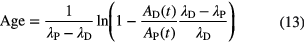
For half-lives longer than hundreds of years it is not feasible to measure accurately the decrease in counting rate over a reasonable length of time. Even with a repeatability of 0.01%, at least a measurement period of 100 years is needed to achieve 0.1% accuracy on a 500 year half-life (equation (34)). In such cases, a measurement of specific activity may be resorted to:
in which AA,Z is the activity and NA,Z is the number of atoms of nuclide AZ of the measured source, NA is the Avogadro number, MA,Z is the molar mass of the isotope, mtot is the total source mass and mZ is the mass of its content of element Z.
The method implies three main stages: absolute measurement of activity concentration [68] in the source material, weighing of the source mass and determination of the isotopic composition. Mass spectrometry is well-suited for the latter, which allows determination of mA,Z/mZ and correcting the total source activity for decays from other isotopes. A difficulty may arise in the mass determination of the base material if the chemical state of the element is not exactly defined. The composition of uranium oxides, for example, varies with the conditions in which it is produced and stored and therefore the oxygen/uranium ratio may vary. The uranium concentration may be investigated with titrations, coulometry, oxygen analysis or isotope dilution mass spectrometry (IDMS) relative to a pure metallic reference material [69].
The mass determination can be skipped by means of a relative measurement of two (or more) isotopes in one material
in which A* represents the mass number of the other isotope(s). Half-life ratios of Pu and U isotopes can be determined from relative peak areas in alpha spectra of quantified mixtures [70].
For a subset of long-lived nuclides having a short-lived parent, e.g. 243Cm-239Pu, 244Cm-240Pu, 249Cf-245Cm and 250Cf-246Cm, the daughter half-life can be determined relatively to the parent half-life by measuring the ingrowth in an initially pure parent source. The daughter-to-parent activity ratio measured after a decay time by a spectrometric technique is roughly proportional to the ratio of their decay constants [71].
Also the activity measurement can be avoided for nuclides appearing in a parent-daughter relationship in a decay chain in secular equilibrium, the activity ratio being constant in this case. Typical examples are the half-life measurements of 234U and 230Th by mass spectrometry of very old materials [72] using the 238U parent as reference, of which the half-life was determined by alpha counting at a defined solid angle [73]. The uncertainty on T1/2(238U) should probably be increased [74], which in turn should be propagated to the daughter nuclides [29].
6. Conclusions
A multitude of techniques have been used to measure nuclear half-lives, their applicability very much depending on the order of magnitude of the value itself. The half-life data are essential for our knowledge of nuclear structure and fundamental natural laws and lead the way to applications in radioactivity measurements, dating techniques and dosimetry. Work is still in progress to measure new data and to confirm or improve existing half-life values. Whereas the quality of the published work has generally improved with time regarding accuracy and traceability, there is still room for improvement in accounting for all factors that may influence the measurement result and providing a complete uncertainty assessment. Underestimation of uncertainties is still a problem today, mostly because the random uncertainty component is often reduced to a minimum and systematic errors and their propagation towards the half-life uncertainty are more difficult to quantify. This has its consequences in scientific debate and societal consequences derived from radioactivity-based techniques.