


ABSTRACT
A ground level enhancement (GLE) is a solar event that accelerates ions (mostly protons) to GeV range energies in such great numbers that ground-based detectors, such as neutron monitors, observe their showers in Earth's atmosphere above the Galactic cosmic ray background. GLEs are of practical interest because an enhanced relativistic ion flux poses a hazard to astronauts, air crews, and aircraft electronics, and provides the earliest direct indication of an impending space radiation storm. The giant GLE of 2005 January 20 was the second largest on record (and largest since 1956), with up to 4200% count rate enhancement at sea level. We analyzed data from the Spaceship Earth network, supplemented to comprise 13 polar neutron monitor stations with distinct asymptotic viewing directions and Polar Bare neutron counters at South Pole, to determine the time evolution of the relativistic proton density, energy spectrum, and three-dimensional directional distribution. We identify two energy-dispersive peaks, indicating two solar injections. The relativistic solar protons were initially strongly beamed, with a peak maximum-to-minimum anisotropy ratio over 1000:1. The directional distribution is characterized by an axis of symmetry, determined independently for each minute of data, whose angle from the magnetic field slowly varied from about 60° to low values and then rose to about 90°. The extremely high relativistic proton flux from certain directions allowed 10 s tracking of count rates, revealing fluctuations of period ≳ 2 minutes with up to 50% fractional changes, which we attribute to fluctuations in the axis of symmetry.
Export citation and abstract BibTeX RIS
1. INTRODUCTION
"One person's data is another person's noise." That cliché aptly describes the relationship between the interplanetary transport of cosmic rays and the mystery of how they are accelerated at the Sun. Modeling solar cosmic ray transport provides our best observational information on how energetic charged particles scatter and diffuse in the solar wind (Meyer et al. 1956; McCracken 1962; Lockwood et al. 1975; Pomerantz & Duggal 1978; Palmer 1982; Debrunner et al. 1984; Smart & Shea 1990; Bieber et al. 2002, 2004; Ruffolo et al. 2006). Yet these same interplanetary transport processes somewhat obscure the connection between the particles observed at Earth and the processes that accelerated them at or near the Sun.
Approximately 15 times per solar cycle, the Sun emits cosmic rays with sufficient energy and intensity to raise radiation levels on Earth's surface markedly above background levels. These events, termed "ground level enhancements" (GLEs), provide an exceptionally clear picture of particle acceleration on the Sun, first because GLE particles travel near the speed of light and thus enable a precise linkage between the particles and the solar source event, and second because they have large mean free paths, and their time profiles are comparatively undistorted by transport processes in the interplanetary medium. Information gained from the observation and analysis of GLEs is clearly pertinent to the field of heliophysics and is also interesting for traditional astrophysics for the challenge it poses to acceleration models (e.g., Roussev et al. 2004).
GLEs are also of practical interest owing to their significance for space weather forecasting and specification. Solar cosmic rays can damage sensitive electronic components aboard spacecraft, and they pose a major radiation hazard to astronauts (Hu et al. 2009). Because GLE particles travel at nearly the speed of light, they provide the earliest indication of an impending radiation storm in some events (Kuwabara et al. 2006). For radiation exposure to air crews and aircraft electronics, GLEs are the only events of relevance, because the lower energy particles that are a major concern in space do not penetrate to aircraft altitudes (Wilson et al. 2003; Lantos 2006). Air routes through the north polar region have multiplied in recent years, because these routes are the most cost-efficient for flights from North America to the Far East (Hanson & Jensen 2002). Radiation hazard is greatest along these routes, because Earth's magnetic field provides little or no protection in polar regions. Fortunately, numerous cosmic ray monitoring stations (neutron monitors) in Canada, Russia, and Greenland are well situated to provide alerts and to monitor radiation hazard on polar airline routes.
This article reports neutron monitor observations of the giant GLE of 2005 January 20, an event that was the most intense observed in nearly half a century and the second largest observed since systematic observations began in the 1930s. Section 2 provides an overview of this giant event in the context of other large GLEs. Section 3 considers the time evolution of the energy spectrum and the total fluence, and Section 4 derives the time evolution of the directional anisotropy. These results are discussed and summarized in Section 5. A companion article (A. Sáiz et al. 2013, in preparation) will report how we perform theoretical modeling of the event, determine the interplanetary scattering conditions encountered by the GLE particles, and derive the particle injection function onto the Sun–Earth magnetic field line.
2. OVERVIEW OF THE GIANT GROUND LEVEL ENHANCEMENT
Over a six-minute span on 2005 January 20, the neutron rate at the sea level station at Terre Adélie, Antarctica increased by about 4200% (i.e., a factor of 43) over the pre-event Galactic background, while the rate at the sea level station at McMurdo, Antarctica increased by a factor of about 2600%, as shown in Figure 1. The increase at the high-altitude (2820 m) station at South Pole (not shown) was even greater, a factor of about 5500%, which we believe is the highest count rate from cosmic sources ever recorded by a neutron monitor. However, this distinction is owing to the unique location of South Pole at both high latitude and high altitude. Corrected to sea level the increase at Pole would have been "only" about 2300%. For clarity, we note that neutrons detected by the instrumentation are secondary neutrons generated from nuclear interactions of primary cosmic rays with Earth's atmosphere. The primary cosmic rays are predominantly protons. This huge increase in the relativistic proton flux was associated with a very strong solar flare (location 14°N 61°W, 1–8 Å X-ray level X7.1 and onset 06:39 UT) and very fast coronal mass ejection (estimated deprojected speed 3675 km s−1; Gopalswamy et al. 2012).
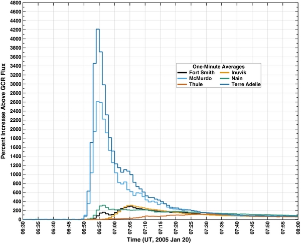
Figure 1. Percentage increases of relativistic solar ions above the Galactic cosmic ray (GCR) background for the giant GLE of 2005 January 20 at six polar, low-altitude neutron monitors, five of which belong to the global Spaceship Earth network. The two-pressure-coefficient procedure has been applied to normalize all stations to sea level. The detected neutrons are secondary cosmic rays generated by nuclear cascades in Earth's atmosphere. The relativistic primary cosmic rays that initiate the cascades are predominantly protons. Because the neutron monitors view different directions in the sky, the major difference between the traces indicates an initially strong anisotropy in relativistic solar protons.
Download figure:
Standard image High-resolution imageAnother notable aspect of this event was its extreme anisotropy. As shown in Figure 1, stations such as Thule and Inuvik had barely experienced any increase at all at the time the intensities at Terre Adélie and McMurdo were peaking. Thule and Inuvik later peaked at a factor of 200% or so. While this is large by recent historical standards, it is more than an order of magnitude smaller than peak intensities recorded in the Antarctic. The near sea level stations displayed in Figure 1 all have similar energy responses governed by atmospheric absorption, rather than by the geomagnetic cutoff. Therefore, the large differences in count rates can be attributed largely to anisotropy of the primary cosmic ray flux.
The 2005 January 20 event is one of a rare (at least in the modern era) class of giant GLEs. Somewhat arbitrarily, we place the threshold for a giant GLE as an increase of 500% over the Galactic background observed by a sea level neutron monitor in any location. In the neutron monitor era, there have been only two giant GLEs, the one under discussion here on 2005 January 20 and the famous event of 1956 February 23 (Meyer et al. 1956). Owing to better time resolution and a better distribution of stations, the 1956 increase would undoubtedly have been larger if observed with the neutron monitor array currently in place. Duggal (1979) reckons the increase would have been 9000% at high latitudes. In addition to a higher peak flux of relativistic particles, the giant GLE of 1956 February 23 had a much higher fluence due to the very long duration of the particle enhancement at Earth.
Table 1 lists the six known giant GLEs together with, for reference, the largest one that did not attain giant status. Four of the giant GLEs were observed by ionization chambers (or Compton–Bennett meters) in the pre-neutron monitor era (Forbush 1946). When compared with neutron monitors, ionization chambers mainly respond to primary particles at higher energies, but the ionization chamber magnitudes listed in Table 1 have been renormalized to correspond to what would have been observed by a favorably situated high-latitude neutron monitor had any existed at the time (Duggal 1979).
Table 1. The Seven Largest Ground Level Enhancements
| Rank | Date | Magnitude | Instrumenta |
|---|---|---|---|
| (%) | |||
| 1 | 1956 Feb 23 | 4600 | NM |
| 2 | 2005 Jan 20 | 4200 | NM |
| 3 | 1949 Nov 19 | 2000 | IC |
| 4 | 1946 Jul 25 | 1100 | IC |
| 5 | 1942 Mar 7 | 750 | IC |
| 6 | 1942 Feb 28 | 600 | IC |
| 7 | 1989 Sep 29 | 360 | NM |
Note. a"NM" denotes neutron monitor. "IC" denotes ionization chamber. IC events have been renormalized to correspond to the increase that a high-latitude neutron monitor would have observed (Duggal 1979).
Download table as: ASCIITypeset image
The GLE of 2005 January 20 has several characteristics of relevance for space weather forecasting and specification. First, the extremely fast rise from background to peak (6 minutes) indicates that a GLE onset can provide an early alert of a major solar particle event. Backtesting studies show that alerts based on GLE onsets typically precede the earliest proton alert issued by NOAA's Space Weather Prediction Center by ∼10–30 minutes (Kuwabara et al. 2006). Though not all large solar proton events (SPEs) are accompanied by GLE, a recent study demonstrated there is a surprisingly sharp threshold in SPE peak intensity, such that the majority of SPE above the threshold are accompanied by GLE for proton energies greater than 40 MeV (Oh et al. 2010).
Second, the extreme anisotropy measured at the beginning of this event shows that anisotropy must be considered when assessing peak radiation dose rate. This is especially true as concerns exposure to the crew and electronics of high-altitude aircraft (Wilson et al. 2003). At the peak of the GLE, some regions of Earth were experiencing near record dose rates from cosmic rays, while at the same time other regions remained at Galactic background levels.
Third, it is important to recognize the large dynamic range of event magnitudes in assessing radiation hazard from solar particles. If observations were available only during the 48 year period from 1957 to 2004, the largest GLE would be the 360% event of 1989 September, and mission planners might seem justified in taking this event as a "worst case" scenario. However, the longer time perspective displayed in Table 1 demonstrates that events more than an order of magnitude greater than this occurred in 1956 and 2005. This is in accord with studies showing that intense solar particle events approximately obey a "log-normal" distribution in peak intensity (Pereyaslova et al. 1996).
This article presents an analysis of neutron monitor data from 11 stations of the Spaceship Earth neutron monitor array (Bieber & Evenson 1995) supplemented by two additional stations as explained below. (Currently there are 12 members of Spaceship Earth, but one station, Peawanuck, Canada, was not operating at the time of the GLE.) All stations except South Pole are near sea level.
High-latitude stations are ideal for studying relativistic solar cosmic rays for several reasons. First, the lowest cutoffs on Earth are in polar regions, and the detector response to a GLE is typically much larger than at mid or low latitudes where the cutoff is higher. Second, the energy response is governed by atmospheric absorption rather than by the geomagnetic cutoff. This means the polar stations have essentially the same energy response, and there is no need to invoke complex analysis procedures to disentangle anisotropy effects from spectrum effects. Abbasi et al. (2008) concluded that these procedures can yield misleading results during the early anisotropic phase of a GLE. Third, the polar stations have excellent directional sensitivity. Figure 2 displays the viewing directions in geographic and in geocentric solar ecliptic (GSE) coordinates of vertically incident particles for each station, computed for 06:53 UT on 2005 January 20 (the time of the peak intensity at South Pole) using the trajectory code described by Lin et al. (1995) to account for the bending of particle trajectories in the geomagnetic field. The trajectory code employs the International Geomagnetic Reference Field together with the Tsyganenko (1989) model of Earth's magnetosphere, and it takes account of variations of the field with season, time of day, and geomagnetic Kp index, which had a value of 2 during 06:00–09:00 UT. For reference, the median rigidity computed for a spectral index of 5.0 (as derived in the next section) is 2.14 GV, corresponding to a kinetic energy of 1.40 GeV. The asymptotic viewing direction depends upon rigidity, so Figure 2 shows that direction for the median rigidity (squares) and the central 80% of the detector response for each station (a range of 1.05 GV to 5.33 GV in rigidity or 0.47 GeV to 4.47 GeV in energy). For this solar spectrum, the central 80% arrive from a region spanning less than 54° at this time. Thus, the dramatic differences in neutron monitor responses displayed in Figure 1 can confidently be attributed to anisotropy of the solar particles in space.

Figure 2. Geographic locations and asymptotic viewing directions of the 13 polar neutron monitors considered in this work at 06:53 UT, the time of peak count rate of the giant GLE of 2005 January 20 (a) in geographic coordinates and (b) in geocentric solar ecliptic (GSE) coordinates. Taking into account the bending of particle trajectories in Earth's magnetic field, each neutron monitor measures the relativistic ion flux from specific asymptotic viewing directions, shown for the median rigidity of 2.14 GV (squares) and for the central 80% of the detector response, 1.05–5.33 GV (lines). Particles would be observed from the directions marked "O" and "X" when moving directly away from or toward the Sun, respectively, along the nominal Archimedean spiral magnetic field direction. The neutron monitors (and two-letter station codes) are Apatity, Russia (AP); Barentsburg, Norway (BA); Cape Schmidt, Russia (CS); Fort Smith, Canada (FS); Inuvik, Canada (IN); Mawson, Antarctica (MA); McMurdo, Antarctica (MC); Nain, Canada (NA); Norilsk, Russia (NO); South Pole, Antarctica (SP); Terre Adélie, Antarctica (TA); Tixie Bay, Russia (TB); and Thule, Greenland (TH).
Download figure:
Standard image High-resolution imageFor this analysis the 11 Spaceship Earth stations were supplemented by two additional stations, Terre Adélie, Antarctica and South Pole, Antarctica. These two stations are not formal members of the Spaceship Earth array for technical reasons (e.g., the number of neutron detector tubes in the station is below the defined Spaceship Earth standard of 18). However, we include them because their observations contribute important special information to the analysis. In the case of Terre Adélie, it is because this station observed the largest percent increase of any station near sea level. South Pole (altitude 2820 m) likewise observed a very large percent increase, though smaller than Terre Adélie when normalized to sea level. In addition, the South Pole station contains special instrumentation that permits us to gain detailed information about the evolution of the particle energy spectrum and fluence. The next section presents our spectral analysis of the South Pole data, and the section that follows presents our detailed analysis of the particle anisotropy.
3. TIME-DEPENDENT ENERGY SPECTRUM
At the time of the giant GLE of 2005 January 20, the South Pole station provided direct information on the spectrum of relativistic solar protons with excellent accuracy and time resolution. This station had both a neutron monitor with three counter tubes in a standard NM64 design and the Polar Bare monitor of six neutron counters with polyethylene moderators but lacking the usual lead producer and polyethylene reflector. The Polar Bare counters are more sensitive to lower energy atmospheric neutrons, and in turn to primary cosmic rays of lower energy, so the Bare/NM64 ratio provides information on the SEP spectrum, after the background Galactic cosmic ray (GCR) rate is subtracted out (Bieber & Evenson 1991; Bieber et al. 2002).
Figure 3 shows the percent increases over the GCR count rate for the Polar Bare and South Pole NM64 detectors, and their ratio, as a function of time. With the aid of yield functions provided by Stoker (1985), the Bare/NM64 ratio can be converted into a spectral index. We assume a differential rigidity spectrum of the power-law form P−γ, where P is the rigidity and γ is the spectral index, with an upper cutoff at 20 GV. The inset scale on the left side of the lower panel shows the spectral index corresponding to various values of the Bare/NM64 ratio. There could be a small systematic error in the estimated spectral index during times of strong anisotropy, due to the different Bare and NM64 asymptotic directions (Bieber & Evenson 1991; Cramp et al. 1997). Nevertheless, in a previous analysis of the GLE of 1989 October 22 (Ruffolo et al. 2006), there was remarkably good agreement for the spectral index as a function of time as inferred from the South Pole detectors and from an independent technique using the worldwide network of neutron monitors at various cutoff rigidities (Cramp et al. 1997).
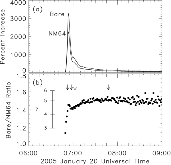
Figure 3. (a) One-minute data of percent increases recorded at the South Pole by a standard (NM64) neutron monitor and a Polar Bare neutron counter that lacks the usual lead shielding. (b) The ratio of percent increases at 1 minute resolution (solid circles) provides an indication of the spectral index γ. The spectrum is initially hard because the most energetic particles arrive first, but it quickly softens due to velocity dispersion. Then at ≈06:55 it suddenly hardens somewhat due to a second dispersive injection peak. Afterward, the spectrum gradually becomes softer to approach a steady state with γ = 5.0. Arrows in the lower panel denote the midpoint of 5 minute intervals for which spectra are displayed in Figure 4. (The final two spectra in Figure 4 are off-scale in the present figure.)
Download figure:
Standard image High-resolution imageThe technique of using bare counters sited near a neutron monitor requires much less modeling effort and can in principle provide a real-time measurement of the spectral index, a feature that has potential application in forecasting peak radiation intensity and fluence at lower energies down to 40 MeV (Oh et al. 2012). This technique for determining the spectral index was especially effective on 2005 January 20 because of the excellent statistics during this giant GLE. In addition, the asymptotic direction for the South Pole station was fortuitously located in the part of the sky with the most intense incoming particle flux. Thus, we can track the spectral variation of relativistic solar protons with unprecedented accuracy and 1 minute time resolution.
As seen in Figure 3(b), the first-arriving protons have a very hard spectrum, because the fastest particles arrive first. The spectrum then becomes softer as the relatively slower particles catch up. Such spectral softening on 2005 January 20 has also been inferred from the count rate ratio between neutron counters without lead and a neutron monitor at SANAE, Antarctica (McCracken et al. 2008) and from neutron monitors with different cutoff rigidities (e.g., Plainaki et al. 2007; Bombardieri et al. 2008). This pattern of softening, referred to as a dispersive onset, is common to all GLEs.
Another common pattern is that the spectral index reaches a steady value at later times, or a value of 5.0 in this case, which is typical for GLEs (Duggal 1979). We interpret that as the spectral index of relativistic proton injection near the Sun. This implies that the median rigidity detected by a sea level polar neutron monitor is 2.1 GV, and the central 80% of the detector response is for ion rigidities of 1.1–5.3 GV, which for protons corresponds to a median kinetic energy of 1.4 GeV and a range of 0.5–4.5 GeV.
What is unique to this event is the sudden spectral hardening between the data points of 06:54 and 06:56 UT after which the overall softening resumes. (Note that throughout this work, when we refer to the data for a minute, such as 06:54, we mean the data for the interval 06:54:00–06:55:00, centered at 06:54:30.) Such hardening was also reported by Plainaki et al. (2007), though with coarser resolution, based on neutron monitors at varying rigidity. This hardening can be interpreted in association with the Polar Bare and NM64 percent increases shown in Figure 3(a). After the main intensity peak at 06:53 UT, there was a second (and much weaker) intensity peak at 07:00 UT. Both peaks exhibit similar dispersion features, with harder spectra before the peak and softer spectra afterward. Thus, we can infer that both intensity peaks were dispersive.
Note that the two solar injections inferred from our analysis do not correspond to two contemporaneous directional distributions with different axes of symmetry (two "fluxes") as proposed by Vashenyuk et al. (2006) or two different types of injections ("pulses") as proposed by McCracken et al. (2008). In our analysis, there is only one axis of symmetry (see Section 4). Furthermore, we consider the second solar injection, inferred from the aforementioned spectral feature at South Pole, to be of the same type as the first injection. In an upcoming companion paper (A. Sáiz et al. 2013, in preparation), we show that the time dependence of the directional distribution of the 2005 January 20 GLE can be explained in terms of known processes of focused transport, without requiring different types of injections at the Sun, and compare the inferred injection function with previously reported results from solar radio and optical observations.
In Figure 4, we compare the intensity spectrum inferred from South Pole observations of relativistic solar protons with the GOES proton spectrum for various time intervals. At early times, velocity dispersion effects are much in evidence as the lower energy protons progressively "catch up" to match the spectrum of the relativistic protons. The energy spectrum inferred from the South Pole station at a median energy of 1.4 GeV after the dispersive onsets is consistent with the GOES spectrum from 54 to 110 MeV. It is steeper than that observed by GOES from 23 to 54 MeV (Figure 4), and even steeper than the spectrum at ∼1 MeV (see Figure 1 of Mewaldt et al. 2005). The steepening with increasing energy, also noted by Mewaldt et al. (2005) (based on spacecraft measurements), Vashenyuk et al. (2005a; based on stratospheric balloon measurements), and Chilingarian & Reymers (2007; based on neutron monitors and an underground muon detector), is a well-known feature of SEP spectra (Ellison & Ramaty 1985).

Figure 4. Spectra of energetic solar protons near Earth as a function of energy, based on data from GOES (lower energy data points) and from the South Pole neutron monitor and Polar Bare neutron counter (lines). Shortly after the onset, there are clear velocity dispersion effects, as the spectrum at lower energies progressively rises to match that at higher energies. The spectrum then steepens at later times. GOES data points are energy channels P4–P7 plotted at the mean energy of the channel. The neutron monitor data point is plotted at a representative (median) energy, and the solid line encompasses the central 80% of the neutron monitor energy response. The dashed portion of the line is an extrapolation of the spectrum. The times of the first four spectra shown are denoted by arrows in Figure 3.
Download figure:
Standard image High-resolution imageThe South Pole neutron monitor was at the low end of worldwide neutron monitor cutoff rigidities, so that it is not surprising that most analyses that included non-polar monitors also inferred steeper spectra. Ryan (2005) inferred a steeper rigidity spectral index of 6.2 using the Mount Washington and Durham neutron monitors (based on the altitude differential; Lockwood et al. 2002), at cutoff rigidities of 1.68 and 1.88 GV, respectively, corresponding to minimum kinetic energies of 0.91 and 1.16 GeV, respectively. Several studies have used fits to data from neutron monitors at various cutoff rigidities. For 41 neutron monitor stations sensitive to solar protons of 1–15 GV, Plainaki et al. (2007) inferred a somewhat steeper index of 7.6 during 06:55–07:00 UT, and Bombardieri et al. (2008) reported a much steeper index of 9.2 during 06:55–07:00 and 7.3–7.7 at later times. Using similar techniques, Vashenyuk et al. (2005b) and Pérez-Peraza et al. (2008) found a harder spectral index of 6.1 at 08:00 UT, from fits to data from 32 neutron monitors. From an analysis of 28 neutron monitors, Matthiä et al. (2009) inferred a soft spectral index of ≈8 during 06:50–07:00 UT and a quite hard index of ≈5 at late times. Based on four monitors ranging from a polar monitor to the Tibet NM at 14.1 GV cutoff rigidity, Miyasaka et al. (2005) measured a spectral index of 4.5 at 07:00 UT and 4.0 + 0.1(P/GV − 1) at 07:10 UT.
The fluence spectrum (the integral of the intensity spectrum over time, for the entire duration of the event), shown in Figure 5, is relevant to estimating the total radiation dosage in space due to relativistic particles during this giant GLE. After correcting for anisotropy effects (described in Section 4) to estimate an omnidirectional average fluence, the relativistic proton fluence inferred from the South Pole data matches well with the GOES measurements at 54 and 110 MeV. Note that the anisotropy effects require a reduction of the South Pole fluence by ∼50% to obtain the omnidirectional average fluence.
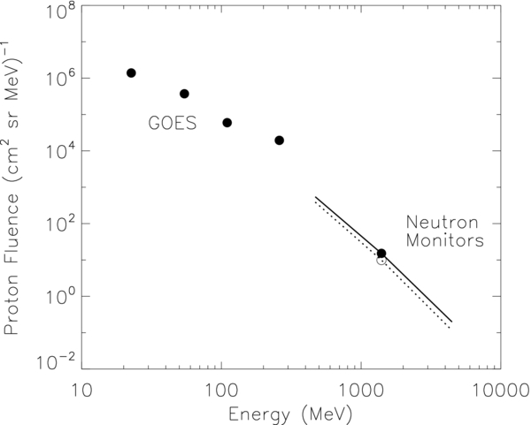
Figure 5. Fluence spectrum of energetic solar protons near Earth as a function of energy, based on data from GOES (lowest four energies), from the South Pole neutron monitor and Polar Bare neutron counter (solid circle and solid line), and an estimate of the omnidirectional average fluence correcting South Pole data for anisotropy effects (open circle and dashed line).
Download figure:
Standard image High-resolution image4. TIME-DEPENDENT DIRECTIONAL DISTRIBUTION
At the start of a GLE, the particle distribution is often highly anisotropic, making it challenging to characterize the directional distribution. The Spaceship Earth network helps greatly to characterize the distribution by using polar neutron monitor stations with different asymptotic directions and similar energy responses. Because the event of 2005 January 20 was a giant GLE, and because of the dense angular coverage of the Spaceship Earth network, we are able to report and characterize one of the most extreme anisotropies ever reported for cosmic rays. From Figure 1, we see that at 06:54 UT, Terre Adélie measured a percentage increase of over 4200% over the GCR background. At that same time, three stations reported percentage increases that were consistent with zero, i.e., either slightly positive or negative and consistent with GCR fluctuations. We can define a maximum-to-minimum anisotropy ratio as the ratio of the highest percentage increase to the lowest, which is attributed to the anisotropy of the directional distribution of relativistic solar protons. For 2005 January 20, we conservatively estimate that the observed peak maximum-to-minimum anisotropy ratio was at least 1000:1.
Next we will describe how we synthesized the data from all Spaceship Earth stations to parameterize the directional distribution of relativistic solar particles near Earth during this giant GLE, and we also examine its time dependence.
4.1. Determination of the Directional Distribution
In this section, we describe how the count rate profiles from individual polar neutron monitor stations were combined to obtain an overall three-dimensional directional distribution of relativistic solar particles in space as a function of time. This distribution is in turn characterized by a time-dependent axis of symmetry and Legendre coefficients (particle density, weighted anisotropy, and second Legendre coefficient), which have physical interpretations and are amenable to further quantitative analysis. Similar analysis techniques have been used previously (Bieber et al. 2002, 2004, 2005; Ruffolo et al. 2006).
Polar neutron monitors at sea level in the Spaceship Earth network have similar spectral responses to primary cosmic rays and a narrow range of asymptotic directions, as discussed in Section 2. Therefore, the percentage increases provide direct information on the directional distribution of relativistic solar protons, with an independent distribution for each minute of data. To combine their data, the total count rate from each of the 13 polar neutron monitors was corrected to a common standard pressure of 760 mm Hg using separate absorption lengths for Galactic and solar particles. For the latter we adopted a standard value of 100 g cm−2 (Duggal 1979). We thereby obtained the GLE-related increase of each count rate over the GCR background, which was modeled by fitting a linear trend to the hourly density. The GLE occurred during the recovery phase of a Forbush decrease due to a preceding solar event, so the linear trend in the GCR flux was unusually strong, at about 5% day−1. According to standard practice in GLE analysis, the flux of relativistic solar particles was expressed in terms of the percentage increase above the GCR background.
We fit the data to directional distributions that are rotationally symmetric about one direction in space. Theories of the interplanetary transport of solar energetic particles (e.g., Ruffolo 1995) generally consider the particle distribution to be axisymmetric about the large-scale magnetic field direction. However, a 2 GV proton has a Larmor radius of about 0.01 AU, on the same order as the coherence length of interplanetary magnetic turbulence (∼0.02 AU), so it is not clear that the particle orbits should be organized around the instantaneous magnetic field measured at the point of observation. We therefore assume axisymmetry, but the direction of the axis of symmetry is optimized to fit the data. When applying this procedure in previous GLE analyses, the station data have indeed been well organized in terms of a pitch angle defined with respect to the axis of symmetry (Bieber et al. 2002, 2004; Ruffolo et al. 2006).
The data were fit using a variety of model functions for the directional distribution of relativistic solar protons in space:


where the {ai} and b are fit parameters, and μ is the cosine of the pitch angle, here defined as the angle between the direction from which the particle arrives and the axis of symmetry. (Note that we use the phrase "axis of symmetry" to refer to a single direction in space, not a bidirectional axis. Sometimes a choice in direction is allowed by an exact or approximate symmetry upon reversal of the axis and the anisotropy; we make the choice that yields a positive anisotropy.) These four functions above represent, respectively, a first-order Legendre polynomial (L1), exponential plus constant (E1), second-order Legendre polynomial (L2), and two exponentials plus constant (E2). The latter two are expected to provide better fits to bidirectional fluxes, if present.
For each polar neutron monitor station and each minute of data, the model under consideration (i.e., one of those in Equation (1)) was used to make a prediction of particle intensity from 10 different asymptotic directions corresponding to the 5-, 15-, ..., 95-percentile rigidities for that station. Percentile rigidities were determined using the spectral index from Section 3, and the computation assumed vertical incidence, which is a good approximation for polar stations owing to the magnetic focusing effect. The 10 intensities were then averaged to yield a prediction for the overall intensity at that station. Next, a chi-square parameter was formed by comparing the predicted with the observed intensity and summing over stations. The free parameters of the model were then obtained via chi-square minimization.
After optimization for each function in Equation (1), we characterize the distribution by five parameters that have physical interpretations, facilitate a comparison between models, and are amenable to further quantitative analysis. These include two parameters to specify the axis of symmetry, and the first three Legendre coefficients about the axis of symmetry: f0, the omnidirectional average intensity or "density," f1, the weighted anisotropy (product of density and dipole anisotropy), and f2, the second Legendre coefficient, related to the curvature of the pitch angle distribution. These are defined as
The quantities fi have the same units as f(μ), in terms of the percentage increase in particle flux over the GCR background.
For the L2 model, fi for i = 0, 1, or 2 is simply equal to ai. The same holds for L1 except that f2 is zero for this model, providing a useful reality check as to whether f2 is really needed. For the E1 and E2 models, fi must be computed by performing the integrals in Equations (2a)–(2c).
Of these four fit functions, E1 (exponential plus constant) was found to provide the best fit to the station data (with the lowest χ2), and also provided a smoothly varying characterization of the directional distribution. Thus time profiles derived from E1 values were adopted for further analysis; these values are shown in Figures 6 and 7. The remaining fits were used in estimating the uncertainties in fi.
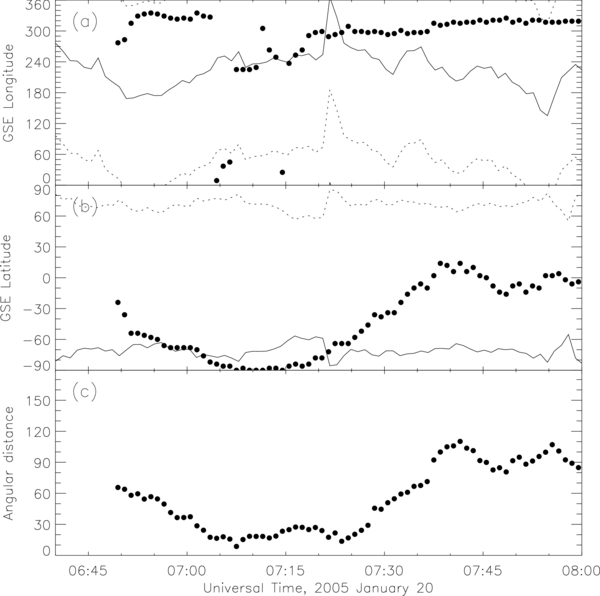
Figure 6. Axis of symmetry of arrival directions of relativistic solar protons (solid circles) in comparison with the magnetic field direction measured by the ACE spacecraft (solid line) and the anti-field direction (dashed line) in terms of (a) GSE longitude, (b) GSE latitude, and (c) angular separation between the axis of symmetry and magnetic field direction (all angles in degrees). Note that the sudden jumps in the longitude of the axis of symmetry correspond to small changes in direction when the latitude was near −90°.
Download figure:
Standard image High-resolution image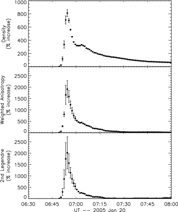
Figure 7. Density, weighted anisotropy, and second Legendre coefficient of the directional distribution of relativistic solar protons near Earth, as inferred independently for each minute of data during the GLE, based on the percentage increase in count rates at 13 polar neutron monitor stations with different asymptotic viewing directions. This GLE had an unusual second peak in the omnidirectional density corresponding to the dispersive spectral feature in Figure 3, which can therefore be attributed to a second solar injection. The increase in weighted anisotropy at the second peak is quite small relative to the increase in density. The weak change in anisotropy may indicate time-dependent interplanetary transport effects or a disturbed interplanetary magnetic configuration that caused a rapid decline in the anisotropy due to the first injection.
Download figure:
Standard image High-resolution image4.2. Axis of Symmetry
Figure 6 shows the direction of the axis of symmetry as a function of time, in terms of the longitude and latitude in GSE coordinates from which particles arrive for a pitch angle of zero (μ = 1). This figure implies that during the early phase of the GLE, when the distribution was highly beamed toward low pitch angles, the highest particle intensity was seen at neutron monitors with southward asymptotic directions, i.e., Terre Adélie and McMurdo (see Figure 2). Note that when the GSE latitude was close to −90°, sudden jumps in longitude correspond to small changes in direction. Thus our inferred axis of symmetry, which was determined independently for each minute of data, is found to vary smoothly as a function of time. Indeed, because of the strong intensity of this giant GLE, we can use this fine (1 minute) cadence and obtain less scatter in the inferred axis of symmetry than in previous analyses (Bieber et al. 2002; Ruffolo et al. 2006; Sáiz et al. 2008).
Qualitatively similar results for the axis of symmetry, based on data from both high- and low-latitude neutron monitors but with 5 minute resolution, were obtained by Bombardieri et al. (2008) for 06:55–07:35 UT. Rather different results from the worldwide network were presented by Plainaki et al. (2007), who reported a particle beam from high southern latitudes before 06:55 UT and low southern latitudes after 07:00 UT, and by Vashenyuk et al. (2006), who used two superimposed axisymmetric distributions to determine that the dominant component(s) jumped from low southern latitudes before 07:05 UT to high southern latitudes during 07:05–07:30 UT and a high northern latitude during 07:30–08:00 UT.
Figure 6 also shows the angular distance between the axis of symmetry from our analysis and the instantaneous magnetic field. It is interesting that this angular difference varies rather smoothly and systematically with time. It started from a large difference of about 60° at 06:48 UT, and over the next 14 minutes (the period of peak flux) it decreased to less than 30°. As noted earlier (see Figure 2), the angular resolution of individual neutron monitor stations is about 30°, so a difference less than that can be taken to indicate close agreement. This trend is similar to that for the GLE of 2003 October 28 (Sáiz et al. 2008), in which case the difference was typically 60°–90° near the start of the GLE. In both events, the magnetic field was often at high southern latitude, and the axis of symmetry of relativistic solar particles was often close to the South Polar direction. The other reported comparison of the axis of symmetry and (averaged) magnetic field direction was for 2000 July 14 (Bieber et al. 2002). The field configuration was rather different, but nevertheless there was an angular difference of over 50° near the time of the intensity peak and during the initial decay, which later decreased.
A novel feature for 2005 January 20 was that the angular difference increased later in the event, and from 07:37 to 08:00 UT it varied over roughly 80°–110°. The start of this increase (up to 07:35 UT) was also reported by Bombardieri et al. (2008). Such an increase at later times was not found in our analyses for the events of 2000 July 14 and 2003 October 28. Possible reasons for both the initial decrease and the later increase will be discussed in the next section.
4.3. Estimation of Uncertainty
Now let us consider the time profiles fi(t) for i = 0, 1, and 2, i.e., the density, weighted anisotropy, and second Legendre coefficient. For their interpretation, as well as accurate least-squares fitting with solar injection and interplanetary transport models, it is important to estimate their uncertainties σi(t) in a reasonable way. Fundamentally, the statistical uncertainties are very low for this giant GLE. We consider that the uncertainties of fi(t) are instead dominated by (1) distribution determination (DD), i.e., estimating a global distribution based on fitting the percentage increases along 13 asymptotic directions, and (2) interplanetary fluctuations (IFs) in density and anisotropy. We estimate both contributions, as described below, and add them in quadrature to obtain σi(t), which like fi(t) is in units of percentage increase.
The DD uncertainties in each time interval were based on the root-mean-squared (rms) deviation of two other fit values from the E1 fit value. For the density and weighted anisotropy, for which values were obtained from three other fits, we removed the "outlier" fit with the greatest deviation, which in many cases would clearly not be considered a reasonable fit. The L1 fit (first-order Legendre expansion) does not estimate f2, which is zero in that model, so for σ2DD we used the rms deviation of L2 and E2 from E1.
During the onset and first peak (0649 to 0656 UT), σiDD was set to the rms deviation itself. However, after 0656 UT, it was found that the ratio of each uncertainty to the weighted anisotropy (σiDD/f1) was reasonably constant for short time periods. Physically, this confirms that the uncertainty mainly arises from the strong anisotropy, whereas a weak anisotropy makes it easier to estimate global quantities from station data. We therefore found it prudent to define time blocks of 3–5 minutes over which to average σiDD/f1, which makes the resulting uncertainties less sensitive to fluctuations in the fits to station data. In particular, it sometimes does happen that all models yield virtually the same values, so without averaging over nearby time intervals, the estimate of σiDD would be unreasonably low and inappropriately constrain fitting to time profiles.
After 0656 UT, boundaries between time blocks were set at five-minute intervals (0700 UT, 0705 UT, etc.). An exception was that the boundary at 0740 UT was replaced by boundaries at 0738 and 0741 UT, corresponding to sudden changes in the deviation between fits to station data. This was when the axis of symmetry was rotating from ∼90°S to the ecliptic plane, evidently a time of unusual directional distributions.
The uncertainties due to IFs were taken to be constant in time, and were estimated based on temporal fluctuations over the time period 0720–0800 UT, during the decay phase, in comparison with short-term linear trend lines. This procedure is sensitive to fluctuations over 1–3 minutes. The results were σ0IF = 0.9, σ1IF = 1.7, and σ2IF = 3.1. This was the dominant contribution to the uncertainty during certain time periods when the DD uncertainty was extremely small (10−3 of the SEP density). The DD and IF uncertainties were added in quadrature to obtain the total uncertainties  , which are included in Figure 7.
4.4. Time-dependent Particle Density and Anisotropy
As a function of time, the (omnidirectionally averaged) particle density shot up very rapidly from its onset at 06:49 to a first peak at 06:54. The weighted anisotropy and second Legendre coefficient were also very high, which is characteristic of a beam that covers a narrow range of angles. During the density decay, there is a shoulder and a minor peak at 07:03. This should be associated with the dispersive spectral feature in Figure 3, and with a second injection of relativistic solar particles from near the Sun.
Another interesting feature of Figure 7 is that for the second peak in the density, there are also peaks in the weighted anisotropy and second Legendre coefficient, but their values relative to the density (i.e., the unidirectional and bidirectional anisotropy) are much lower than for the first peak. Somehow the second injection seems to have much less anisotropy than the first, only a few minutes earlier. We aim to understand this in further work, when we will fit the data in Figure 7 by comparing them with simulations of the interplanetary transport of relativistic solar particles.
4.5. Ten-second Count Rates at Various Stations
Finally, one more interesting feature of Spaceship Earth observations of this giant GLE is that count rates were so high that they can be binned over sub-minute timescales and still show statistically meaningful variations. Several of the Spaceship Earth neutron monitor stations were equipped to provide 10 s count rates, as shown in Figure 8 for selected neutron monitors and also the South Pole bare counters. Note that the Polar Bare peak is higher than the South Pole neutron monitor peak in Figure 3(a), while the neutron monitor peak is higher in Figure 8. The reason is that Figure 3(a) displays a ratio of percent increases relative to the Galactic background, whereas Figure 8 displays a pure count rate.

Figure 8. Ten-second count rates for selected Spaceship Earth neutron monitor stations, and the South Pole neutron monitor (N) and bare counters (B). During the giant GLE of 2005 January 20, at times the count rates were so high that statistically significant variations can be seen from one 10 s interval to the next. There were numerous fluctuations over periods of 2 minutes or longer, involving fractional changes of up to 50% in the count rate (note the logarithmic scale). At these times the overall density and level of anisotropy varied much more slowly, and on the whole these fluctuations can be attributed to minor changes in the axis of symmetry, i.e., the beaming direction of particles in space.
Download figure:
Standard image High-resolution image
For the high-altitude South Pole neutron monitor, during the peak the 10 s count rate exceeded 104, yielding a fractional statistical accuracy of ∼0.01, whereas the flux had fractional changes of up to 50% from one 10 s interval to the next during the initial rise. This is one of the few times that neutron monitors have ever provided data on cosmic ray variations with sub-minute resolution (see also Bieber et al. 1990). Because 10 s count rates were collected at various stations, they may provide further information on the directional distribution.
Figure 8 shows that after a rapid rise and/or rapid decline associated with the peak count rate, each detector observes substantial fluctuations in the count rate, typically over periods of 2 minutes or longer. The amplitude and frequency decline noticeably after ≈07:18 UT or so, together with the overall decline in anisotropy (see Figure 7). Whenever there are sufficient counting statistics, it is seen that there are essentially no fluctuations with sub-minute periods. Fluctuations are sometimes found to be similar at stations with nearby asymptotic directions (see Figure 2).
Now let us consider the origin of the short-time fluctuations in station data, e.g., at McMurdo from 06:56 to 07:18 UT, when fractional changes were as strong as 50% per minute. These clearly do not represent changes in the average density of cosmic rays in space. According to Figure 7 the inferred omnidirectional density of cosmic rays in space varied rather smoothly from one minute to the next, with a fractional change of at most several percent (at 07:04 UT, which we attribute to a second injection of relativistic solar particles). Similarly, the fluctuations cannot be attributed to rapid changes in the level of anisotropy in the interplanetary particle distribution, because this anisotropy mostly exhibited a smooth decrease with time. However, as noted above, the amplitude of the fluctuations seems to be associated with the level of anisotropy. Therefore the fluctuations seen in Figure 8 for data from individual stations can be attributed to changes in the axis of symmetry of a highly anisotropic interplanetary directional distribution, or changes in how that distribution maps onto various geographical locations at Earth.
Note that South Pole bare counters and South Pole neutron monitors have similar short-time fluctuations, i.e., their ratio varies over longer timescales (see Figure 3). Thus, the fluctuations seem to be independent of the particle energy. The passage of particles through Earth's magnetic field, and the asymptotic directions, are quite dependent on particle energy, so we consider it unlikely that the rigidity-independent South Pole fluctuations can be attributed to temporal changes in how the interplanetary distribution maps to geographic locations at Earth. Given the extreme anisotropy that was sometimes over 1000:1, minor fluctuations in the axis of symmetry of the interplanetary particle distribution can account for the fluctuations in the station data. We therefore attribute the short-time fluctuations in neutron monitor count rates to minor fluctuations in the axis of symmetry of the directional distribution in interplanetary space.
5. DISCUSSION AND CONCLUSIONS
This work presents observations of the giant GLE of 2005 January 20, one of the strongest GLEs ever observed with electronic detectors. We have analyzed data from the Spaceship Earth network of 13 polar neutron monitors to determine the spectral index, directional distribution, time–intensity, and time–anisotropy profiles of relativistic solar particles during this event.
We determine the spectral index from data at a single station (South Pole) with both bare counters and a neutron monitor. Using the ratio of counters at a single station removes various systematic effects. The South Pole count rate for this event was so high that we obtained statistically accurate estimates of the spectral index on a minute-by-minute basis. We observe energy dispersion, i.e., spectral hardening leading up to the main peak in solar particle intensity, which is a common feature of GLEs, indicating that faster particles arrive first from a distant source, i.e., the Sun. What is unusual in this event is a second dispersive feature just after the time of peak intensity (Figure 3), which corresponds to a second peak in the omnidirectional density (Figure 7). We therefore attribute the second peak to a distinct injection of relativistic protons from near the Sun. Multiple solar injections were possibly seen for the GLE of 2003 October 28 (Bieber et al. 2005; Sáiz et al. 2008) but were not seen during various other GLEs studied by the Spaceship Earth network or its predecessors (Bieber et al. 2002, 2004; Ruffolo et al. 2006).
The temporal changes in density and anisotropy during 2005 January 20 appear consistent with a second solar injection. Considering the increase above the decaying density and weighted anisotropy from the main injection, the additional anisotropy at the time of the second injection appears to be much weaker than during the main injection. A lower additional anisotropy might be associated with a temporal change in transport conditions for particles in the second injection relative to the first. On the other hand, there could also be time-independent transport conditions that cause a particularly rapid decline in anisotropy for particles from the main injection. Examples include disturbed magnetic conditions, such as a magnetic bottleneck (Bieber et al. 2002) or a closed interplanetary magnetic loop (Ruffolo et al. 2006). A quantitative analysis with precision modeling is needed to distinguish between these possibilities, which will be the subject of a forthcoming paper.
We have also analyzed the systematic time variation of the axis of symmetry of the directional distribution, i.e., the beaming direction, with respect to the local magnetic field. In addition to the event of 2005 January 20, there were two other events, 2000 July 14 and 2003 October 28, for which the axis of symmetry from Spaceship Earth or its predecessors was compared with the local interplanetary magnetic field (Bieber et al. 2002; Sáiz et al. 2008). In all three cases, the published results indicate an angular difference of over 50° at early times which decreased later in the event. (In our unpublished results for 2001 April 15, a similar pattern was found.) This may be a general feature of GLEs. Note also that for 2005 January 20 the axis of symmetry underwent further rotation back to the ecliptic plane during the intensity decay, a phenomenon for which we do not have a clear explanation.
The strong beaming of the interplanetary distribution of relativistic solar protons, with a maximum-to-minimum anisotropy that was sometimes greater than 1000:1 on 2005 January 20, can be understood in terms of the focused transport of SEPs along the interplanetary magnetic field. However, it is noteworthy that the particles are apparently beamed along a direction different from the local interplanetary magnetic field for all three GLEs. A contributing factor for 2005 January 20 may be the uncertainty in determining the axis of symmetry, given that our method assumes axisymmetry, and during most of this event the directions of the axis of symmetry and the magnetic field were far to the South, where we have relatively sparse coverage in terms of asymptotic directions. Indeed, during the start of the event there were strong signals in only a few neutron monitors. However, we consider it unlikely that the angular deviation is entirely due to modeling uncertainty, because the inferred axis of symmetry varied smoothly and systematically with time, not exhibiting sudden swings as might be expected for an ambiguous or highly uncertain optimization. Furthermore, for the event of 2000 July 14 the axis of symmetry was close to the equatorial plane, where we had dense coverage of asymptotic directions.
To explain why the axis of symmetry can be different from the local magnetic field direction, previous work (e.g., Bieber et al. 2002) noted that particles of such high rigidity have a large gyroradius and sample magnetic fields at different locations where the magnetic field could deviate from the locally measured value. During the GLE of 2005 January 20, the magnetic field was rather steady (see Figure 6) so the locally measured value does not seem to be anomalous. Thus, we consider effects of magnetic field variations at locations offset from Earth and not sampled by magnetometers near Earth. Note that the particle orbit samples the magnetic field up to a gyrodiameter 2RLsin θ from the location of interest in a direction perpendicular to the guiding field, where RL is the Larmor radius and θ is the pitch angle. For the median rigidity protons observed by Spaceship Earth at times of spectral index 5.0 (as seen for this GLE at late times), we have 2RL ∼ 0.02 AU, on the order of the coherence length of magnetic turbulence in the solar wind (Jokipii & Coleman 1968). However, during times of strong beaming, most particles have θ close to zero and a gyrodiameter much smaller than 2RL. This makes it less likely that a field-aligned beam became substantially misaligned by sampling a different magnetic field during excursions perpendicular to the guiding field. At the same time, the gyrowavelength parallel to the guiding field is 2πRLcos θ, or ≈2πRL when there is strong parallel beaming, which is ∼0.06 AU for the above median rigidity. While a particle beam along a guiding (large-scale) magnetic field is expected to follow the field as it varies gradually, a sudden change in the magnetic field over a distance much smaller than the gyrowavelength can cause field-aligned particles to suddenly obtain higher pitch angles. Such a change in the magnetic field need not have been very close to the observer, because a non-aligned beam can persist for some distance before it is spread out by interplanetary scattering (which was weak during this event) and realigned by adiabatic focusing (which is much weaker near Earth than near the Sun).
Furthermore, this can qualitatively explain why such deviations are stronger near the start of a GLE. According to our determination of the spectral index, the nominal median rigidity at the start of the 2005 January 20 GLE was 8.16 GV, compared with 2.14 GV later in the event. For such protons, the gyrowavelength was nearly four times greater. Thus the protons observed at the start of the GLE were sensitive to magnetic field changes over such distance scales along a substantial portion of their trajectory from the Sun, making them more susceptible to changes in beaming direction compared with particles later in the event. In contrast, the effects of perpendicular drifts and diffusion are usually thought to be weak compared with focused transport effects (see, e.g., Ruffolo et al. 1998), and it is hard to imagine how they could cause a relativistic particle beam to become substantially misaligned from a guiding magnetic field.
There are various analyses of GLEs in the literature that consider the time profiles of count rates of individual stations, sometimes attributing secondary peaks at a single station to fresh injections of particles from the Sun. Our finding that minor peaks in the count rate at an individual station, as seen in Figure 8, were usually not associated with changes in the omnidirectional density or the level of anisotropy in interplanetary space—or with particle acceleration at the Sun—serves as an example that single-station data can be misleading. The same can be said for SEP data from a spacecraft instrument that only views a narrow set of directions in space, which may be the case if the spacecraft does not rotate. A combined analysis that incorporates a wide range of viewing directions provides a much clearer picture of the distribution of solar particles in interplanetary space.
In summary, from our analysis of data from 13 polar neutron monitors for the giant GLE of relativistic solar protons on 2005 January 20, we conclude the following.
- 1.This giant GLE produced the highest count rate increase ever observed by a neutron monitor (about 5500%, at South Pole), and the second-highest count rate increase at sea level (about 4200%, at Terre Adélie), where the highest was on 1956 February 23.
- 2.Using the neutron monitor and Polar Bare counters at South Pole, we infer the time dependence of the spectral index of relativistic solar protons. Both the main peak and a weaker second peak in the omnidirectional particle density correspond to dispersive onsets, and are qualitatively consistent with two distinct injections of relativistic protons near the Sun followed by interplanetary transport to Earth.
- 3.Using the Spaceship Earth network supplemented to comprise 13 polar neutron monitor stations with different asymptotic particle arrival directions, we have characterized the three-dimensional directional distribution of relativistic solar protons.
- 4.The relativistic solar protons were strongly beamed, at times with a maximum-to-minimum anisotropy greater than 1000:1.
- 5.The directional distribution is characterized by an axis of symmetry. The angular distance between this axis of symmetry and the magnetic field direction was initially about 60°, then decreased to low values, and then increased to about 90° during the later decay phase.
- 6.With such a high-particle density in interplanetary space, this event provided a rare opportunity to observe statistically meaningful variations in the cosmic ray flux at sub-minute timescales. In 10 s count rates, after a rapid rise and/or rapid decline, individual neutron monitor stations recorded further fluctuations with up to 50% fractional changes over 1 minute. These can be attributed mainly to fluctuations in the axis of symmetry of the directional distribution, not in the omnidirectional density or the level of anisotropy.
- 7.For the second peak in the density of relativistic solar protons, the change in anisotropy associated with the particle injection appears to be much weaker than for the main peak. This may be due to either time-dependent transport conditions or a disturbed magnetic configuration such as a magnetic bottleneck or loop causing a particularly rapid decline in the anisotropy due to the main injection.
We thank our colleagues at IZMIRAN (Russia), the Polar Geophysical Institute (Russia), and the Australian Antarctic Division for furnishing data. Terre Adélie data were kindly provided by the French Polar Institute (IPEV, Brest) and by Paris Observatory. This solar event was a SHINE campaign event, and we thank Allan Tylka for making his summary and bibliography for this event available through the SHINE Web site. We thank the ACE/MAG team and the ACE Science Center for providing magnetometer data online, and the GOES program for online energetic proton data. This research was partially supported by the US National Science Foundation (grants ANT-0739620 and ANT-0838839) and the Thailand Research Fund.