


ABSTRACT
We present the results of 938 speckle measures of double stars and suspected double stars drawn mainly from the Hipparcos Catalog, as well as 208 observations where no companion was noted. One hundred fourteen pairs have been resolved for the first time. The data were obtained during four observing runs in 2014 using the Differential Speckle Survey Instrument at Lowell Observatory's Discovery Channel Telescope. The measurement precision obtained when comparing to ephemeris positions of binaries with very well-known orbits is generally less than 2 mas in separation and 0 5 in position angle. Differential photometry is found to have internal precision of approximately 0.1 mag and to be in very good agreement with Hipparcos measures in cases where the comparison is most relevant. We also estimate the detection limit in the cases where no companion was found. Visual orbital elements are derived for six systems.
Export citation and abstract BibTeX RIS
1. INTRODUCTION
Observations of binary stars have traditionally played an important role in our knowledge of stellar structure and evolution, and this remains a vital field primarily because of the increased resolution that can be obtained for imaging of binaries as well as the precision in radial velocity and metallicity measurements that can be derived from stellar spectra. Over the last two decades, this has resulted in a dramatic increase in the number of systems that can be studied with multiple techniques. A few examples of resolving close binaries and deriving precise relative astrometry include the work of Hummel et al. (1995, 1998) on spectroscopic binaries with both the Mark III and Navy Optical Interferometers, a similar program at the Palomar Testbed Interferometer (Muterspaugh et al. 2010b and references therein), the comprehensive study of Torres et al. (2009) on α Aurigae, the extremely productive speckle program of Mason, Hartkopf, and their collaborators (Mason et al. 2013), the speckle program of Tokovinin and his collaborators in the Southern Hemisphere (Tokovinin et al. 2015 and references therein), the work of Balega et al. (2013), and our own work at the WIYN and Gemini telescopes (Horch et al. 2011a, 2011b, 2012, 2015). In addition, both the Hipparcos Catalog and the Geneva-Copenhagen spectroscopic survey give a ready list of binaries, some of which will become important if future observations can be used to establish their orbital parameters. This is a particularly favorable situation for the derivation of stellar masses of sufficient quality to make progress on the understanding of the dependence of mass on parameters such as metallicity and age. In the best case of a resolved binary that also is a double-lined spectroscopic system, a distance measure independent of Hipparcos can be derived.
The structure and physical parameters of binary and multiple stars are informative from a statistical point of view regarding star formation theories, as shown most recently in papers such as Raghavan et al. (2010), Tokovinin (2014a, 2014b), and Riddle et al. (2015). In addition, it has been realized in the last couple of years that a significant number of stars that host exoplanet systems also have a stellar companion (e.g., Horch et al. 2014; Kane et al. 2014; Lillo-Box et al. 2014), although there is evidence that the presence of stellar secondaries is suppressed relative to the field at smaller separations (Wang et al. 2014a, 2014b). High-precision astrometric measurements of binaries and multiple stars that are relatively close to the Sun are a key prerequisite to exploring these issues.
With these facts in mind, we have started a new program of speckle observations of double stars at Lowell Observatory's Discovery Channel Telescope (DCT), a 4.3-m telescope recently commissioned by the observatory and its partner institutions. The observing program is largely an extension of work previously done by two of us (E.H. and M.E.) at the WIYN 3.5 m telescope at Kitt Peak, together with other collaborators. However, we also have an interest in the current program to identify and study nearby and young binaries, whereas the WIYN program focused more on differentiating between the thin and thick disk samples of binaries. The primary sources of potential targets remain the Hipparcos and Geneva-Copenhagen Catalogs. We detail here the first year of observations on the program, which used the Differential Speckle Survey Instrument (DSSI).
2. OBSERVATIONS
The DSSI was on the telescope on four occasions during 2014: two nights in March, two in June, eight nights from September 30 to October 7, and four more in November for a total of 16 nights, of which approximately five were used for binary star observations reported here. The instrument is described in Horch et al. (2009), and the subsequent upgrade to the use of electron-multiplying CCD cameras instead of the original low-noise, large format CCD chips is described in Horch et al. (2011a). A number of other observational programs were executed during the four runs, including high-resolution imaging of minor planets and follow-up observations for the Kepler satellite mission; those will be discussed in future papers. In between the spring and fall runs, the instrument was used at the Gemini North telescope, thus it was disassembled and packed for shipping both to and from Hawaii. The instrument was designed with portability in mind, so this procedure is relatively straight-forward, but it does mean that the plate scale calibrations for the later two runs at the DCT can be expected to be slightly different than for the first two runs. The seeing for the observations at the DCT presented here ranged from 0.6 to 1.2 arcsec, with an average value of 0.8 arcsec.
All observations taken here consisted of sets of 1000 short exposure images of the target star, with each image being 40 ms in duration. In the case of some fainter objects, two or three such sets were taken and co-added in the analysis phase. A 128 × 128 subarray was used for all observations discussed here; this gave DSSI a field of view of about 2.4 × 2.4 arcsec at the DCT. Prior to observing, the target list was put into groups of two to several stars that had sky positions within a few degrees of one another. These were then generally observed in order of increasing right ascension starting when the first target was near the meridian. An unresolved source taken from the Bright Star Catalogue was used as a calibration object for the purposes of determining the speckle transfer function for each group of science targets, and placed within the group based on its right ascension. In this way, the zenith distance of all observations in the group was kept to a minimum.
Figure 1 shows two representations of the data set for the systems where a companion was detected; in Figure 1(a), the data are plotted in terms of the magnitude difference obtained as a function of the measures separation, and in Figure 1(b), the magnitude differences are plotted as a function of the total (system) magnitude appearing in the Hipparcos Catalog (ESA 1997). These figures are comparable to previous work with the instrument at the WIYN 3.5 m telescope (e.g., Horch et al. 2011a), and are effectively semi-log plots since the y-axis is proportional to the log of the brightness ratio. In particular, the envelope of points in Figure 1(a) shows that, starting at small separations, the sensitivity to the magnitude difference of companions rises sharply, but a "knee" appears at a separation of approximately 0.1 arcsec (Δm of 3–4 mag), and at larger separations the sensitivity continues to rise, albeit at a more modest pace. One can also note that there are some systems with measured separations below the nominal diffraction limit at the DCT of about 0.04 arcsec (at 692 nm). This is possible due to the fact that the DSSI takes images in two filters simultaneously. As discussed in Horch et al. (2011b) (Paper III of this series), the two-color analysis permits us to distinguish between atmospheric dispersion and the presence of a companion below the diffraction limit. Generally, to minimize the effect of atmospheric dispersion, we observed the targets at an airmass of less than 2.
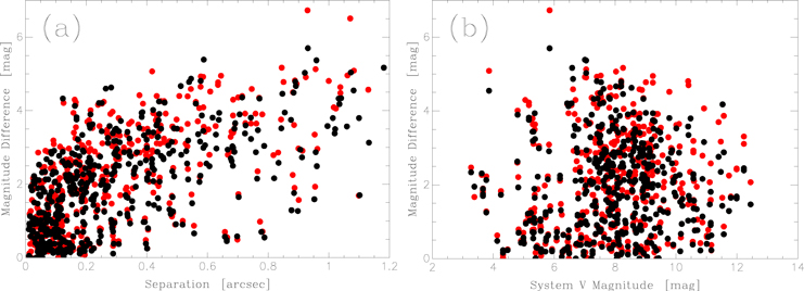
Figure 1. (a) Magnitude difference as a function of separation for the measures listed in Table 3. (b) Magnitude difference as a function of system V magnitude for the measures listed in Table 3. In both plots, the red circles are measures taken with the 692 nm filter and black circles are measures in the 880 nm filter.
Download figure:
Standard image High-resolution image3. DATA REDUCTION AND ANALYSIS
3.1. Determination of the Pixel Scale and Orientation
In our work at the WIYN telescope with DSSI, we constructed a slit mask for use in the determination of the pixel scale and orientation at that telescope. We were able to attach the mask to the tertiary mirror baffle support and, with the help of WIYN staff, were able to easily mount and remove the mask with minimal loss of observing time. This essentially follows the example of the CHARA and USNO speckle programs, and is generally considered the most reliable method for precise scale and orientation calibration for speckle measures. However, at the DCT, we do not yet have such a system in place since the tertiary mirror is located inside the instrument cube and therefore inaccessible. As a result, we were forced in 2014 to rely on a group of calibration binaries during each run. This limits the precision of our measures somewhat, especially at the larger separations that we report here, since the scale in arcseconds per pixel is multiplied by the separation in pixels to obtain the final separation. However, we will show that there is no evidence for a systematic offset in separations we obtain. In the future, we plan to develop a system by which a calibration mask can be placed inside the DSSI camera itself. This would allow us to make a robust scale determination from first principles regardless of the telescope with which DSSI is used, and will be important to ensure the long-term consistency of our speckle measures.
On each run, we selected a small number of binaries with extremely well-known orbits with which to measure the scale. We required that the the orbits used include recent data and that the ephemeris uncertainties in position angle and separation be less than or equal to 05 and 1 mas respectively. Table 1 shows the final scale in mas per pixel and the offset angle between celestial coordinates and the pixel axes that were applied on each run. Because we observed very few objects in November for this project, we did not have the opportunity to observe scale objects, so the results from the September/October run were applied.
Table 1. Final Values for the Pixel Scale and Orientation
| Run | Channel A | Channel A | Channel B | Channel B |
|---|---|---|---|---|
| Offset Angle | Scale | Offset Angle | Scale | |
| Mar | 545 |
18.433 mas/pix | −577 |
20.486 mas/pix |
| Jun | 527 |
18.249 mas/pix | −562 |
20.345 mas/pix |
| Sep/Oct | 539 |
18.781 mas/pix | −539 |
20.029 mas/pix |
| Nov | 539 |
18.781 mas/pix | −539 |
20.029 mas/pix |
Download table as: ASCIITypeset image
Table 2 shows the objects used to obtain the results in Table 1 for each run. The columns give (1) the month of the run, (2) the Washington Double Star (WDS) number of the binary used, (3) the discoverer's designation, (4) the Hipparcos number, (5) the Besselian year of our observation, (6–9) the observed minus calculated residual in position angle and separation for both the A and B cameras, and (10) the reference for the orbit used to do the calculation. Although we did not take data on scale calibration objects in November, we did however measure the scale in another way, albeit at lower precision. We took a sequence of 1 s exposures on a bright star, offsetting the telescope in various directions in between the exposures. By measuring the centroid position of the star in each case and calculating the shift between frames, we were able to compare this to the number of arcseconds we had moved the telescope, and thereby determine both the scale and offset angle. This method allowed us to conclude that the scale and offset angles in November were consistent with those derived for the September/October run. Therefore, we used the latter to all of the November data.
Table 2. Orbits and Residuals Used in the Scale Determination
| Run | WDS | Discoverer | HIP | Besselian | ΔθA | ΔρA | ΔθB | ΔρB | Orbit Reference |
|---|---|---|---|---|---|---|---|---|---|
| Designation | Year | (°) | (mas) | (°) | (mas) | ||||
| Mar | 15232 + 3017 | STF 1937AB | 75312 | 2014.2189 | −0.3 | +3.0 | −0.2 | +1.2 | Muterspaugh et al. (2010a) |
| 2014.2244 | +0.2 | −1.7 | 0.0 | +1.3 | |||||
| 15278 + 2906 | JEF 1 | 75695 | 2014.2189 | +0.3 | +1.7 | +0.4 | +1.5 | Muterspaugh et al. (2010a) | |
| 2014.2244 | +0.5 | −3.3 | +0.2 | −5.3 | |||||
| 17080 + 3556 | HU 1176AB | 83838 | 2014.2190 | −0.6 | +0.2 | −0.5 | 0.0 | Muterspaugh et al. (2010a) | |
| Jun | 15232 + 3017 | STF 1937AB | 75312 | 2014.4594 | −0.2 | −0.3 | 0.0 | −0.5 | Muterspaugh et al. (2010a) |
| 15278 + 2906 | JEF 1 | 75695 | 2014.4594 | −0.1 | +0.1 | 0.0 | +0.5 | Muterspaugh et al. (2010a) | |
| Sep/Oct | 04136 + 0743 | A 1938 | 19719 | 2014.7584 | 0.0 | +0.2 | 0.0 | +0.2 | Muterspaugh et al. (2010a) |
| 19490 + 1909 | AGC 11AB | 97496 | 2014.7577 | 0.0 | −0.1 | −0.1 | +0.7 | Muterspaugh et al. (2010a) | |
| 21145 + 1000 | STT 535AB | 104858 | 2014.7552 | +0.4 | +0.2 | +0.4 | +0.5 | Muterspaugh et al. (2008) | |
| 22409 + 1433 | HO 296AB | 111974 | 2014.7608 | −0.1 | −1.9 | −0.1 | −5.7 | Muterspaugh et al. (2010a) | |
| 2014.7636 | −0.3 | +1.8 | −0.2 | +1.5 |
Download table as: ASCIITypeset image
Two things may be noted from Table 2. First, for each run shown, the average residual is zero (or very near zero) for both position angle and separation in the A camera, and for the position angle in the case of the B camera. However, the average residual is not zero for the separation residuals for the B camera. Specifically, for the five measures used in March, the average residual is −0.26 mas, and for September/October, it is −0.56 mas. This is because in this channel, DSSI is known to have a scale distortion which is dependent on position angle that is related to the positioning of one of the optical components in the optical train. More information about this distortion can be found in Horch et al. (2009, 2011a). For the data presented here, we assumed that the offset of this element was the same as what we have measured at the WIYN telescope. If this parameter varied slightly from the WIYN value, it would be possible to obtain a non-zero residual for this purpose. By varying the scale, one can minimize, but not eliminate, an average residual in this case. This is not an issue for position angle or the scale in the A camera, which does not have this problem. Another way to check that the scale is not influenced by this is to compare results from the A and B camera for all observations; we show that these do not have a significant difference in Section 3.3.1. We conclude that the variations we see in Table 2 are likely dominated by random error.
Second, we may use the values in Table 2 to derive a simple estimate of the measurement precision by calculating the standard deviation of each type of residual in Columns 6–9, if we assume that the error in the ephemeris position is negligible. In this case we obtain σθ,A = 0.31 ± 006 and σθ,B = 0.26 ± 005 in position angle and σρ,A = 1.7 ± 0.4 mas and σρ,B = 2.5 ± 0.5 mas in separation. Averaging, this indicates internal precision of ∼03 in position angle and ∼2 mas in separation.
3.2. Speckle Data Reduction
The reduction of science data followed the same sequence as described in previous papers in this series (e.g., Horch et al. 2011a, 2015). The autocorrelation function is formed for each frame of the speckle exposure, and these are summed. Near-axis subplanes of the image bispectrum are also calculated for each frame and summed. Then, using the method of Meng et al. (1990), we form an estimate of the phase function for the object in the Fourier plane. We combine this with the modulus of the power spectrum (derived from the autocorrelation function deconvolved by the observation of a point source) to have a full estimate of the Fourier transform of the object. This is low-pass filtered with a Gaussian function where the width is chosen to give an FWHM that is similar to that of a diffraction-limited point-spread function. Finally, to obtain a diffraction-limited reconstructed image, the result is inverse-transformed. To give an indication of the typical quality of the results, reconstructed images for two objects, HDS 2143 and CHR 74, are shown in Figure 2. Orbits for each object are presented later in the paper.
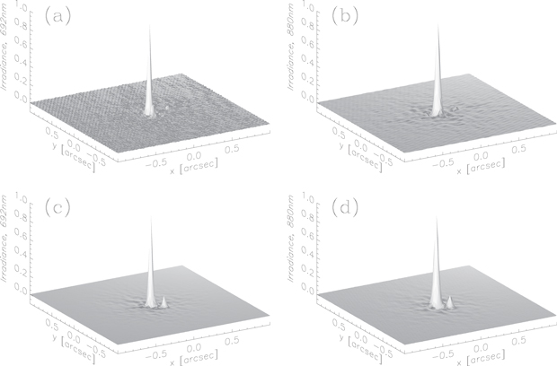
Figure 2. Reconstructed images of two targets. (a) HDS 2143 = HIP 74649 in the 692 nm filter. (b) HDS 2143 = HIP 74649 in the 880 nm filter. (c) CHR 74 = HIP 91118 in the 692 nm filter. (d) CHR 74 = HIP 91118 in the 880 nm filter.
Download figure:
Standard image High-resolution imageThe reconstructed image is then examined for companions visually. If a companion is noted, then the pixel location of the secondary peak is noted and used as the starting position for a fitting program that performs a weighted least-squares fit to the object's power spectrum. In the case of a successful fit, the measure has been added to our main list of results. If, on the other hand, a companion is not noted visually, we then compute a detection limit as a function of separation from the target. More about this process is given in the Section 3.4.
3.3. Double Star Measures
In Table 3, we present our measures of double stars. The columns are as follows: (1) the WDS number (Mason et al. 2001), which also gives the right ascension and declination for the object in 2000.0 coordinates; (2) the Aitken Double Star (ADS) Catalog number, or if none, the Bright Star Catalogue (i.e., Harvard Revised (HR)) number, or if none, the Henry Draper Catalog (HD) number, or if none the Durchmusterung (DM) number of the object; (3) the Discoverer Designation; (4) the Hipparcos Catalog number; (5) the Besselian date of the observation; (6) the position angle (θ) of the secondary star relative to the primary, with north through east defining the positive sense of θ; (7) the separation of the two stars (ρ), in arcseconds; (8) the magnitude difference (Δm) of the pair in the filter used; (9) the center wavelength of the filter; and (10) the FWHM of the filter transmission. The measures have not been precessed from the dates shown. One hundred fourteen objects in the table have no previous detection of the companion in the fourth Catalog of Interferometric Measures of Binary Stars (Hartkopf et al. 2001b); we propose discoverer designations of Lowell-Southern Connecticut (LSC) 2-115 here. (These numbers begin at 2 because LSC 1Aa1, Aa2 = HIP 103641 was discovered in previous work in collaboration with Lowell (Horch et al. 2012).)
Table 3. DCT Double Star Speckle Measures
| WDS | HR, ADS | Discoverer | HIP | Date | θ | ρ | Δm | λ | Δλ |
|---|---|---|---|---|---|---|---|---|---|
| (α,δ J2000.0) | HD, or DM | Designation | (2000+) | (°) | ('') | (mag) | (nm) | (nm) | |
| 00012 + 1358 | BD+13 5195 | LSC 2 | 96 | 2014.7580 | 184.5 | 0.2168 | 2.35 | 692 | 40 |
| 2014.7580 | 184.6 | 0.2166 | 1.59 | 880 | 50 | ||||
| 00067 + 0839 | ... | LSC 3 | 551 | 2014.7580 | 15.9 | 0.5730 | 4.07 | 692 | 40 |
| 2014.7580 | 15.7 | 0.5755 | 3.16 | 880 | 50 | ||||
| 00087 − 0213 | HD 406 | LSC 4 | 700 | 2014.7553 | 109.0 | 0.9242 | ... | 692 | 40 |
| 2014.7553 | 108.7 | 0.9210 | ... | 880 | 50 | ||||
| 00121 + 5337 | ADS 148 | BU 1026AB | 981 | 2014.7581 | 318.6 | 0.3436 | 1.02 | 692 | 40 |
| 2014.7581 | 318.6 | 0.3447 | 0.93 | 880 | 50 | ||||
| 00126 + 4419 | HD 802 | LSC 5 | 1011 | 2014.7554 | 314.8 | 0.5856 | 4.92 | 692 | 40 |
| 2014.7554 | 314.7 | 0.5878 | 5.39 | 880 | 50 |
Notes.
aQuadrant ambiguous. bQuadrant inconsistent with previous measures in the fourth Interferometric Catalog of Hartkopf et al. (2001b). cThird component noted, but above 1.2 arcsec. dThis object was used in the determination of the pixel scale and detector orientation, so only the magnitude difference measure is reported here.Only a portion of this table is shown here to demonstrate its form and content. Machine-readable and Virtual Observatory (VOT) versions of the full table are available.
Download table as: Machine-readable (MRT)Virtual Observatory (VOT)Typeset image
3.3.1. Astrometric Accuracy and Precision
Since we have a camera that takes data in two colors simultaneously, we can use the independent results in each channel to make a determination regarding the intrinsic precision of our measures. In Figure 3, we show the residuals obtained when subtracting the position angle and separation obtained in Channel B (880 nm) from those obtained in Channel A (692 nm). Figure 3(a) shows the position angle result for all measures in Table 3; these show a negligible relative offset: the average difference obtained is 0.04 ± 0.11 degrees, and the standard deviation obtained from all measures is 2.24 ± 0.07 degrees. The latter is expected to increase as the separation decreases, since the linear measurement uncertainty orthogonal to the separation subtends a larger angle at smaller separations. If only measures with separations larger than 0.1 arcsec are included, then the average difference remains consistent with zero, namely −0.08 ± 0.12 degrees, and the standard deviation decreases to 0.51 ± 0.09 degrees.
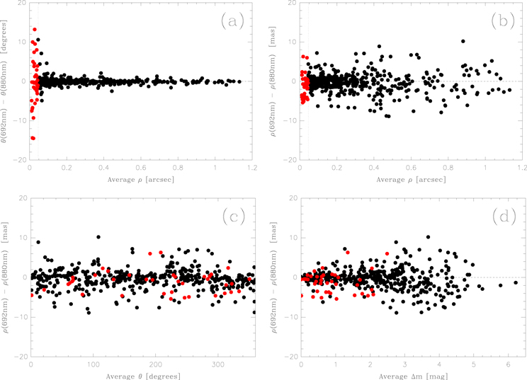
Figure 3. Measurement differences between the two channels of the instrument plotted as a function of measured separation, position angle, or magnitude difference. (a) Position angle (θ) differences as a function of average separation. (b) Separation (ρ) differences as a function of average separation. In both plots, the dotted vertical line at the left marks the average diffraction limit of the two wavelengths used, and squares indicate measures below the diffraction limit. (c) Separation differences as a function of average position angle. (d) Separation differences as a function of average magnitude difference. In all plots, the filled red circles indicate measures below the diffraction limit.
Download figure:
Standard image High-resolution imageIn Figures 3(b)–(d), the separation differences are shown as a function of average separation, average position angle, and average magnitude difference respectively. From the entire data set, we obtain an average difference between the channels of −0.39 ± 0.12 mas with a standard deviation of 2.57 ± 0.09 mas. Such an offset might arise from the distortion in Channel B of the instrument, which is known to depend on position angle. However, when plotting the residuals as a function of position angle (Figure 3(c)), we see no clear trend. This is good evidence that the distortion model applied is appropriate for DCT data; if this were not the case, then the residuals would have a sinusoidal trend with two complete periods covered in the full range of 360° in position angle. On the other hand, when plotting the data as a function of average separation or magnitude difference, we see that there is a slight negative trend to the residuals for the measures reported below the diffraction limit (Figure 3(b)) and for measures where the magnitude difference is large (Figure 3(d)). For measures above the diffraction limit and having average Δm < 3, we obtain an average A–B difference of = −0.07 ± 0.11 mas, with a standard deviation of 1.96 ± 0.08 mas. Overall, we conclude that the scale and offset angles applied to the data yield no significant offsets between the channels for the bulk of the measures presented, with the caveat that below the diffraction limit and at large magnitude difference, there may be small systematic offsets particularly in separation. It is also clear that at large magnitude difference, the internal precision of the measures degrades. The average difference in separation for measures below the diffraction limit is −1.20 ± 0.44 mas with standard deviation of 2.78 ± 0.31 mas, and for measures with average magnitude difference greater than 3.0 we have an average difference of −0.95 ± 0.34 mas with a standard deviation of 3.60 ± 0.24 mas. Thus, given the data at hand, the systematic offset in separation appears to be on the order of perhaps 1 mas in both cases. This effect has so far not been noticed at WIYN, and should be studied further when more data at the DCT is available.
Nonetheless, for the purposes of the present paper we have not corrected for this possible source of error and we will use the intrinsic precision for all measures derived from the first separation difference mentioned, 2.57 ± 0.09 mas. Since this is a difference formed from two independent measures of (assumed) equal precision, the standard deviation obtained will be  times the precision of an individual measure. So, we estimate that the intrinsic precision of separation measures is
  mas. This in turn suggests that the position angle precision should follow the relation
  which has value 02 at a separation of approximately 0.5 arcsec; this is reasonably consistent with Figure 3(a).
There are a number of binaries observed that have orbits of relatively high quality in the Sixth Catalog of Visual Orbits of Binary Stars (Hartkopf et al. 2001a) that were not used in the determination of the scale. We may use these to further judge the intrinsic accuracy and precision of the measures in Table 3. A listing of these objects is given in Table 4, together with the orbit information. We studied the position angle and separation values separately. To be used for the position angle study, we required that the orbit have published uncertainties in the orbital parameters, and that for the epoch of our observation, the propagated uncertainty in position angle was less than or equal to 4°. For the separation study, we again required published uncertainties in the orbital parameters, and that the propagated uncertainty in separation for the epoch of observation was less than or equal to 4 mas. Figure 4 shows the observed minus ephemeris residuals in both parameters plotted as a function of separation. In this case, to make the plots clearer, we have averaged the observed result in both channels prior to plotting. There are no noticeable offsets or trends in either coordinate. The average residual in position angle is 0.16 ± 0.21 degrees, whereas the average residual in separation is −0.90 ± 0.94 mas with standard deviation of 4.96 ± 0.66 mas. Many of the objects with the largest residuals are also those with smallest separations. The internal repeatability study suggests that the precision of these measures is probably not very different than those of larger separations. It is therefore possible that the uncertainties for the orbital parameters for these objects may be slightly underestimated. If, on the other hand, we consider only those objects with separations greater than 0.1 arcsec, then the average residual in separation is 0.47 ± 0.81 mas. Here, the standard deviation of residuals is 2.91 ± 0.57 mas, with the average ephemeris uncertainty being 1.96 mas. If we subtract the latter figure from the former in quadrature, we can obtain another estimate of the intrinsic measurement precision, where the result is 2.15 ± 0.80 mas, which is consistent with the value obtained from comparing the A and B channels.
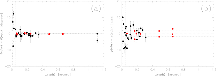
Figure 4. Observed minus ephemeris differences in position angle and separation when comparing the measures presented here with orbital ephemerides of objects having an orbit in the Sixth Orbit Catalog of Hartkopf et al. (2001a) with the quality criteria described in the text. (a) Position angle residuals. In this plot, the dotted–dashed curves mark the position angle error expected from a linear measurement error of 1.82 mas, the derived value for a single-channel measurement. (b) Separation residuals. The dotted–dashed line is drawn at 1.82 mas. In both plots, the dotted vertical line at the left of the plot marks the average of the diffraction limits in the 692 nm and 880 nm filters, and the error bars indicate the uncertainties in the ephemeris position based on error propagation of the published uncertainties in the orbital elements. Filled red circles indicate the observations used to determine the scale, and are not used in the derivation of the statistics mentioned in the text for this study.
Download figure:
Standard image High-resolution imageTable 4. Ephemeris Positions and Residuals Used in the Astrometric Accuracy Study
| WDS | Discoverer | HIP | Besselian | θeph | ρeph |

|

|
Orbit Reference |
|---|---|---|---|---|---|---|---|---|
| Designation | Year | (°) | ('') | (°) | (mas) | |||
| 00121 + 5337 | BU 1026AB | 981 | 2014.7581 | 319.1 ± 1.8 | 0.3474 ± 0.0088 | −0.5 | (−3.3) | Hartkopf et al. (1996) |
| 00507 + 6415 | MCA 2 | 3951 | 2014.7554 | 136.6 ± 9.8 | 0.0477 ± 0.0019 | (−3.6) | −8.0 | Mason et al. (1997) |
| 01057 + 2128 | YR 6Aa,Ab | 5131 | 2014.7555 | 297.9 ± 2.2 | 0.1057 ± 0.0064 | −0.3 | (−1.4) | Horch et al. (2010) |
| 01072 + 3839 | A 1516AB | 5249 | 2014.7554 | 24.9 ± 4.4 | 0.1479 ± 0.0024 | (+4.6) | +5.4 | Hartkopf et al. (2000) |
| 01083 + 5455 | WCK 1Aa,Ab | 5336 | 2014.7581 | 42.3 ± 1.6 | 1.1127 ± 0.0475 | −4.1 | (−41.0) | Drummond et al. (1995) |
| 02022 + 3643 | A 1813AB | 9500 | 2014.7582 | 130.2 ± 12.4 | 0.0393 ± 0.0036 | (+2.3) | +0.7 | Hartkopf et al. (2000) |
| 02157 + 2503 | COU 79 | 10535 | 2014.7582 | 38.6 ± 0.1 | 0.1933 ± 0.0014 | +0.6 | +2.0 | Muterspaugh et al. (2010a) |
| 02396 − 1152 | FIN 312 | 12390 | 2014.7557 | 87.0 ± 0.3 | 0.0864 ± 0.0004 | +0.4 | −3.6 | Docobo & Andrade (2013) |
| 02424 + 2001 | BLA 1 Aa,Ab | 12640 | 2014.7556 | 95.4 ± 3.0 | 0.0540 ± 0.0013 | −0.8 | −0.8 | Mason (1997) |
| 04044 + 2406 | MCA 13Aa,Ab | 19009 | 2014.7583 | 123.4 ± 15.1 | 0.0377 ± 0.0034 | (−8.3) | −8.5 | Mason et al. (1997) |
| 04357 + 1010 | CHR 18Aa,Ab | 21402 | 2014.7584 | 120.9 ± 1.4 | 0.1553 ± 0.0059 | +0.2 | (+0.1) | Lane et al. (2007) |
| 04382 − 1418 | KUI 18 | 21594 | 2014.7584 | 3.1 ± 1.6 | 1.1105 ± 0.0218 | 0.0 | (−28.3) | Hartkopf et al. (1996) |
| 06098 − 2246 | RST 3442 | 29234 | 2014.7587 | 146.0 ± 3.3 | 0.1131 ± 0.0029 | −1.5 | +4.7 | Hartkopf et al. (1996) |
| 06154 − 0902 | A 668 | 29705 | 2014.7587 | 341.8 ± 4.0 | 0.2439 ± 0.0075 | −1.8 | (+1.4) | Hartkopf et al. (1996) |
| 06171 + 0957 | FIN 331Aa,Ab | 29850 | 2014.7586 | 197.2 ± 5.6 | 0.0565 ± 0.0014 | (+2.3) | −1.2 | Hartkopf et al. (1996) |
| 08468 + 0625 | SP 1AB | 43109 | 2014.2183 | 196.0 ± 0.6 | 0.2706 ± 0.0018 | −1.3 | +2.3 | Hartkopf et al. (1996) |
| 13100 + 1732 | STF 1728AB | 64241 | 2014.2189 | 12.1 ± 0.02 | 0.2210 ± 0.0019 | 0.0 | (−36.7) | Muterspaugh et al. (2010a) a |
| 64241 | 2014.4620 | 12.1 ± 0.02 | 0.1611 ± 0.0020 | −0.2 | (−43.7) | Muterspaugh et al. (2010a) a | ||
| 13396 + 1045 | BU 612AB | 66640 | 2014.2189 | 243.7 ± 1.1 | 0.2245 ± 0.0026 | −1.1 | +0.7 | Mason et al. (1999) |
| 66640 | 2014.4621 | 245.6 ± 1.1 | 0.2171 ± 0.0026 | −0.9 | +0.7 | Mason et al. (1999) | ||
| 17217 + 3958 | MCA 47 | 84949 | 2014.2190 | 90.7 ± 1.4 | 0.0213 ± 0.0005 | +12.3 | +5.9 | Muterspaugh et al. (2008) |
| 84949 | 2014.4623 | 125.4 ± 0.3 | 0.0474 ± 0.0006 | +2.7 | +3.3 | Muterspaugh et al. (2008) | ||
| 17247 + 3802 | HSL 1Aa,Ab | 85209 | 2014.2190 | 244.2 ± 2.2 | 0.0255 ± 0.0005 | +3.3 | −9.1 | Horch et al. (2015) |
| 85209 | 2014.4623 | 38.7 ± 4.0 | 0.0120 ± 0.0003 | +7.3 | +10.2 | Horch et al. (2015) | ||
| 19091 + 3436 | CHR 84Aa,Ab | 94076 | 2014.7549 | 295.0 ± 1.9 | 0.0553 ± 0.0016 | −1.8 | +4.4 | Farrington et al. (2014) |
| 20329 + 4154 | BLA 8 | 101382 | 2014.7551 | 161.4 ± 0.1 | 0.0155 ± 0.0001 | −7.5 | −4.6 | Torres et al. (2002) |
| 21109 + 2925 | BAG 29 | 104565 | 2014.7552 | 146.4 ± 1.3 | 0.2454 ± 0.0009 | −1.0 | +3.4 | Balega et al. (2010) |
| 21135 + 1559 | HU 767 | 104771 | 2014.7551 | 0.3 ± 2.1 | 0.1098 ± 0.0025 | +2.6 | −0.5 | Hartkopf et al. (1996) |
| 21501 + 1717 | COU 14 | 107788 | 2014.7552 | 65.3 ± 0.2 | 0.2345 ± 0.0014 | −0.2 | −1.6 | Muterspaugh et al. (2010a) |
| 22388 + 4419 | HO 295AB | 111805 | 2014.7636 | 334.1 ± 0.2 | 0.3093 ± 0.0028 | +0.4 | −2.3 | Horch et al. (2015) |
| 22535 − 1137 | MCA 73 | 113031 | 2014.7552 | 114.7 ± 6.1 | 0.0781 ± 0.0040 | (−6.4) | −2.7 | Mason et al. (2010) |
| 23052 − 0742 | A 417AB | 113996 | 2014.7552 | 91.7 ± 0.9 | 0.1953 ± 0.0016 | +0.7 | −3.5 | Hartkopf et al. (1996) |
| 23411 + 4613 | MLR 4 | 116849 | 2014.7608 | 140.5 ± 1.8 | 0.1262 ± 0.0013 | −1.7 | −2.6 | Hartkopf et al. (1996) |
| 116849 | 2014.7636 | 140.5 ± 1.8 | 0.1262 ± 0.0013 | −1.2 | −2.4 | Hartkopf et al. (1996) | ||
| 23529 − 0309 | FIN 359 | 117761 | 2014.7609 | 181.1 ± 5.1 | 0.0659 ± 0.0017 | (+5.0) | −8.8 | Mason et al. (2010) |
| 117761 | 2014.7637 | 181.0 ± 5.2 | 0.0659 ± 0.0017 | (+5.0) | −8.9 | Mason et al. (2010) |
Note.
aAlthough the separation uncertainty meets the criteria discussed in the text, this object will probably need an orbit refinement after passing through periastron, as discussed in Horch et al. (2015), so we have not used the separations here. This does not affect the position angles, as it is an edge-on system.Download table as: ASCIITypeset image
3.3.2. Photometric Precision
We investigate the photometric precision of our measures by first defining a parameter which should approximately scale with the ratio of the measured separation to the size of the isoplanatic angle, as we have in previous papers in this series. Let this parameter, which we call q', equal the seeing value for the observation multiplied by the measured separation of the pair. (Since the seeing should be roughly proportional to the inverse of the isoplanatic angle, the desired ratio is obtained, up to a scaling factor.)
In Figure 5(a) we plot the difference between the magnitude difference we obtain for each measure at 692 nm appearing in Table 3 and the value of the magnitude difference appearing in the Hipparcos Catalog (ESA 1997). This comparison is limited since the center wavelength of the Hipparcos Hp filter is significantly bluer than either filter we have used. Nonetheless, the closest comparison we can make is with our 692 nm data. The plot shows what we have seen in previous papers, namely that the residuals are flat out to a value of q' = 0.6 arcsec2 and that, at larger values, the most reliable measures tend to have positive residuals. This is expected since, as the separation becomes larger, there will be a loss of correlated speckles between the primary and secondary speckle patterns, and therefore a systematically large value of the magnitude difference will be obtained. For this reason, if the measure has a q' value larger than 0.6 arcsec2, then we have not included the magnitude difference in Table 3.
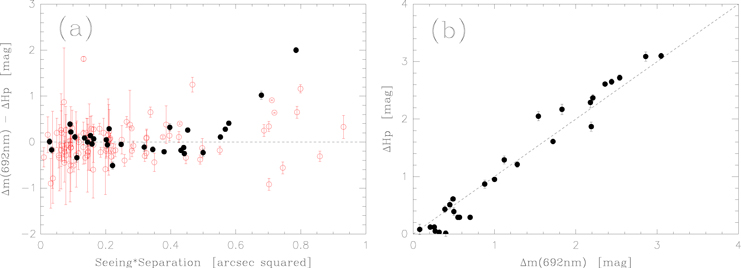
Figure 5. A comparison of the differential photometry presented in Table 1 with Hipparcos differential photometry. (a) The difference in Δm between our measure at 692 nm and the ΔHp value appearing in the Hipparcos Catalog as a function of the parameter q' = seeing times separation discussed in the text. Stars with indications of variability and/or no B − V value in the Hipparcos Catalog are not considered. Filled black circles indicate those systems with a B − V < 0.6 and an uncertainty in the ΔHp value of less than 0.10 mag. Open red circles have no color cut and no cut in ΔHp. (b) A plot of the ΔHp value as a function of the magnitude difference in Table 1 for those systems with B − V color less than +0.6 and  mag. In both plots, the error bars are the uncertainties appearing in the Hipparcos Catalog.
Download figure:
Standard image High-resolution imageFigure 5(b) shows the ΔHp values with the lowest uncertainties plotted as a function of the Δm(692 nm) value we have obtained. We have eliminated objects which are giants, have indications in the Hipparcos Catalog of variability, and those with B − V > 0.6. The plot shows a basically linear trend of slope near 1, as expected. The scatter about the mean line is higher than, e.g., Horch et al. (2011a), but this is probably still due to the fact that we are comparing results in a blue filter with one in a red filter, whereas in the 2011 work, there were many measures at 562 nm, a much better match to Hp. There are a number of examples in Table 3 of objects that were observed twice; the average difference in the magnitude difference obtained for these objects is 0.10 ± 0.01 in the 692 nm filter and 0.13 ± 0.02 in the 880 nm filter. As these are subtractions of independent measures of the same intrinsic precision, we can estimate the internal repeatability of our magnitude differences of  mag, very similar to results we have obtained at the WIYN and Gemini North telescopes.
Similarly, there are two objects, HIP 75312 and HIP 75695, that we observed on three separate occasions. The average standard deviation of the magnitude difference in each filter for these two cases is 0.068 at 692 nm and 0.081 at 880 nm. Assuming this is not a significant difference, then we can average all values regardless of filter to obtain 0.075 ± 0.012, in excellent agreement with the derived value from objects observed twice.
3.4. Nondetections
There were 104 objects that were observed with both filters under good conditions and the images obtained were judged to be of high quality, but did not show any evidence of a companion. In these cases, we can estimate the limiting magnitude difference as a function of separation from the central star from the reconstructed images. Our method for doing so was described in Horch et al. (2011a), but briefly, we form annuli centered on the peak of the central star of width 0.1 arcsec and separated by 0.1 arcsec. In each annulus, we locate all local maxima and local minima. We compute the average value and standard deviation of the local maxima. We also compute the standard deviation of the absoluted value of the local minima. Typically, this value is similar to that of the local maxima, so we average these to obtain a more robust estimate of the standard deviation of all extrema, and then consider the 5σ detection limit to be the average value plus five times this "average" standard deviation.
Figure 6 shows the result of this calculation for two objects: one where no companion was detected, HIP 77986, which is the Be star 4 Her, and one where a companion was detected, namely HIP 113690 = LSC 104. (The first measurement of this system appears in Table 3.) In these plots, a detection-limit curve is traced out using twelve concentric annuli, from 0.1 to 1.2 arcsec. The curve plotted is a cubic spline interpolation, and it assumes that the curve has limiting Δm of zero at the diffraction limit. In the case of LSC 104, we see a point representing a local maximum at separation 0.13 arcsec that is below the detection limit curve, indicating that this peak has greater than 5σ significance. In contrast, for HIP 77896, no peaks appear below the curve, indicating that no second source was detected.

Figure 6. Detection limit analysis for HIP 77986 = 4 Her as described in the text. (a) The result in the 692 nm filter. (b) The result in the 880 nm filter. For comparison, the detected double star HIP 113690 = LSC 104. (c) The result in the 692 nm filter. (d) The result in the 880 nm filter. Note that in both plots for this object, a secondary is clearly detected below the 5σ curve (i.e., it is more than a 5σ result statistically) at a separation of approximately 0.13 arcsec.
Download figure:
Standard image High-resolution imageIt is interesting to compare the shape of these detection limit curves with Figure 1(a). The envelope of the points in Figure 1(a) has a similar form, which indicates that, for high-quality observations, DSSI observations generally will not miss secondaries that fall within the area defined by the typical detection limit curves, such as those seen in Figures 6(c) and, (d). Table 5 gives our final list of high-quality non-detections, with the detection limit obtained at 0.2 arcsec. This value is just above the "knee" in the curve, which gives a good reference point for the rest of the curve.
Table 5. High-quality Nondetections and 5σ Detection Limits
| (α,δ J2000.0) | HIP | Date | 5σ Det. Lim. | 5σ Det. Lim. | Notesa |
|---|---|---|---|---|---|
| (WDS format) | (2000+) | (692 nm) | (880 nm) | ||
| 01320+5712 | 7141 | 14.7581 | 4.43 | 3.61 | YSC 25; previous Δm = 4.92 (698 nm) |
| 01473+0659 | 8319 | 14.7555 | 3.32 | 3.27 | OCC 46; Hipparcos suspected double |
| 02282+2940 | 11486 | 14.7582 | 4.45 | 4.33 | YSC 1; previous sep of 90 mas (2003) |
| 02330+1910 | 11855 | 14.7557 | 3.47 | 3.80 | Hipparcos suspected double |
| 02366+1227 | 12153 | 14.7557 | 3.18 | 4.14 | MCA 7; G-C spectroscopic binaryb; |
| ephemeris sep. near diff. lim. | |||||
| 03233−0748 | 15776 | 14.7556 | 3.74 | 3.79 | Probable thick disk member. |
| 03234+3059 | 15781 | 14.7557 | 4.01 | 4.03 | Hipparcos suspected double |
| 03538+0652 | 18224 | 14.7583 | 4.23 | 4.12 | Hipparcos suspected double |
| 04042+4232 | 18994 | 14.7583 | 4.47 | 4.20 | Probable thick disk member |
| 04163+3644 | 19915 | 14.7584 | 4.29 | 3.96 | YSC 128; previous sep 32 mas (2010) |
| 04501−1548 | 22467 | 14.7584 | 3.82 | 4.26 | HDS 622; previous sep 1.1 arcsec, now off chip? |
| 05018+2639 | 23402 | 14.7585 | 4.35 | 4.23 | BAG 21Ca, Cb; previous sep 24 mas (2000) |
| 05100−0704 | 24037 | 14.7585 | 4.29 | 4.48 | Probable thick disk member |
| 05271−1154 | 25486 | 14.7585 | 3.74 | 4.41 | G-C spectroscopic binary |
| 05315+5439 | 25880 | 14.7586 | 4.51 | 4.12 | Probable thick disk member |
| 05541+5703 | 27885 | 14.7586 | 4.37 | 4.22 | G-C spectroscopic binary |
| 05559−2141 | 28047 | 14.7559 | 3.04 | 2.70 | G-C spectroscopic binary |
| 07338+1324 | 36771 | 14.2237 | 3.18 | 3.08 | G-C spectroscopic binary |
| 08246−0443 | 41214 | 14.2237 | 4.29 | 3.79 | G-C spectroscopic binary |
| 10020+5150 | 49162 | 14.2242 | 4.33 | 4.19 | Hipparcos suspected double |
| 13235+6248 | 65336 | 14.2243 | 4.08 | 4.03 | YSC 131; previous sep. of 30 mas |
| 65336 | 14.4620 | 4.15 | 3.86 | G-C spectroscopic binary | |
| 13282+5035 | 65698 | 14.4620 | 4.05 | 4.24 | YSC 48; previous Δm = 4.62 |
| 14273+5319 | 70674 | 14.2243 | 4.19 | 3.96 | G-C spectroscopic binary |
| 70674 | 14.4620 | 3.95 | 4.03 | G-C spectroscopic binary | |
| 15310+1725 | 75978 | 14.2244 | 3.73 | 3.60 | Hipparcos suspected double |
| 15418−0627 | 76865 | 14.2244 | 3.71 | 4.14 | Hipparcos suspected double |
| 15555+4234 | 77986 | 14.7547 | 4.21 | 4.22 | Be Star: 4 Her |
| 15565+3722 | 78077 | 14.2245 | 4.16 | 3.98 | Hipparcos suspected double |
| 16335−1410 | 81067 | 14.4622 | 3.03 | 3.79 | HDS 2341; previously unresolved by Tokovinin et al. (2010) |
| 16347−0414 | 81170 | 14.4623 | 3.02 | 3.51 | Known SB1, probably below the diff. lim. |
| 16391−2759 | 81521 | 14.4622 | 3.00 | 3.55 | G-C spectroscopic binary |
| 16392+6819 | 81539 | 14.4623 | 3.59 | 3.30 | YSC 113; previous Δm = 4.93 |
| 16552−1118 | 82794 | 14.4595 | 2.99 | 2.81 | G-C spectroscopic binary |
| 17135+5529 | 84264 | 14.2245 | 4.19 | 3.97 | G-C spectroscopic binary |
| 17140−1641 | 84295 | 14.4596 | 3.02 | 2.98 | Hipparcos suspected double |
| 17163−0337 | 84484 | 14.4596 | 3.25 | 3.46 | Hipparcos suspected double |
| 17176+0145 | 84600 | 14.4596 | 3.17 | 3.50 | G-C spectroscopic binary |
| 17198+0208 | 84780 | 14.4596 | 3.73 | 4.09 | Hipparcos suspected double |
| 17198−0403 | 84784 | 14.4596 | 3.12 | 3.90 | G-C spectroscopic binary |
| 17307−1321 | 85691 | 14.4596 | 2.93 | 2.88 | Hipparcos suspected double |
| 17358−1550 | 86104 | 14.4596 | 3.25 | 2.82 | Hipparcos suspected double |
| 17370+6845 | 86201 | 14.4623 | 3.07 | 3.10 | G-C spectroscopic binary |
| 17402−0209 | 86476 | 14.4597 | 3.61 | 3.59 | Hipparcos suspected double |
| 17419−0944 | 86606 | 14.4597 | 2.89 | 2.65 | HDS 2503; below diff. lim.? |
| 17426−0451 | 86677 | 14.4597 | 3.07 | 3.21 | Hipparcos suspected double |
| 17505+0205 | 87318 | 14.4598 | 3.31 | 3.51 | Hipparcos suspected double |
| 18323+1625 | 90877 | 14.7548 | 4.43 | 3.69 | HDS 2630; previous sep. 210 mas |
| 18325−1556 | 90897 | 14.7575 | 3.37 | 3.67 | Hipparcos suspected double |
| 18342−1742 | 91032 | 14.7575 | 3.56 | 3.02 | Hipparcos suspected double |
| 18342+1428 | 91034 | 14.7548 | 4.38 | 4.16 | Hipparcos suspected double |
| 18354−1916 | 91135 | 14.7575 | 3.36 | 3.43 | Hipparcos suspected double |
| 18365+0907 | 91217 | 14.7548 | 4.31 | 4.42 | G-C spectroscopic binary |
| 18386+2038 | 91410 | 14.7548 | 4.69 | 3.92 | Hipparcos suspected double |
| 18395−1840 | 91486 | 14.7575 | 3.06 | 3.14 | Hipparcos suspected double |
| 18430+2948 | 91789 | 14.7548 | 4.05 | 2.70 | Hipparcos suspected double |
| 18442+0456 | 91908 | 14.7548 | 4.32 | 4.28 | G-C spectroscopic binary |
| 18383−0107 | 91384 | 14.7575 | 4.02 | 3.19 | G-C spectroscopic binary |
| 18444+6156 | 91921 | 14.7575 | 4.30 | 4.39 | G-C spectroscopic binary |
| 18460−1936 | 92079 | 14.7575 | 3.22 | 2.59 | Hipparcos suspected double |
| 19053−0131 | 93743 | 14.7576 | 4.46 | 4.26 | G-C spectroscopic binary |
| 19060+0719 | 93787 | 14.7549 | 4.52 | 4.14 | Hipparcos suspected double |
| 19116−0933 | 94297 | 14.7549 | 3.64 | 4.18 | Hipparcos suspected double |
| 19175+0415 | 94806 | 14.7549 | 4.30 | 4.19 | Hipparcos suspected double |
| 19218+2840 | 95187 | 14.7576 | 4.10 | 4.33 | Hipparcos suspected double |
| 19279+2421 | 95702 | 14.7576 | 3.81 | 3.98 | Hipparcossuspected double |
| 19396+2645 | 96704 | 14.7576 | 4.06 | 3.91 | Hipparcos suspected double |
| 19413+1157 | 96859 | 14.7577 | 4.09 | 4.34 | Hipparcos suspected double |
| 19449−1034 | 97157 | 14.7550 | 3.56 | 3.82 | Hipparcos suspected double |
| 19455−0701 | 97216 | 14.7550 | 3.91 | 4.16 | G-C spectroscopic binary |
| 19500+3158 | 97579 | 14.7550 | 3.69 | 3.71 | HDS 2823Aa, Ab; previously unresolved by |
| Balega et al. (2007) and Horch et al. (2011a) | |||||
| 19530+3846 | 97846 | 14.7550 | 3.84 | 3.39 | Probable thick disk member |
| 20007+2243 | 98505 | 14.7550 | 4.16 | 4.12 | HD 189733; no previous measures in 4th IC |
| (Exoplanet host star) | |||||
| 20085+1541 | 99210 | 14.7578 | 4.22 | 4.28 | G-C spectroscopic binary |
| 20092+0715 | 99282 | 14.7578 | 3.91 | 4.10 | Hipparcos suspected double |
| 20097−0308 | 99332 | 14.7550 | 4.10 | 4.37 | Hipparcos suspected double |
| 20195+3844 | 100214 | 14.7578 | 4.43 | 4.32 | Wolf–Rayet Star: WR 139 = V444 Cyg, |
| previously unresolved by 4 observers | |||||
| 20224+1655 | 100468 | 14.7577 | 4.49 | 4.02 | Hipparcos suspected double |
| 20233−0027 | 100550 | 14.7550 | 4.39 | 3.79 | Hipparcos suspected double |
| 20290+1020 | 101034 | 14.7577 | 4.66 | 3.94 | Hipparcos suspected double |
| 20292+0248 | 101043 | 14.7578 | 4.16 | 3.94 | Hipparcos suspected double |
| 20393+2906 | 101928 | 14.7578 | 4.71 | 4.22 | G-C spectroscopic binary |
| 20446+1333 | 102380 | 14.7551 | 3.98 | 3.90 | Hipparcos suspected double |
| 20467+1846 | ... | 14.7551 | 3.22 | 3.31 | YR 28; previous sep. 81 mas (decreasing) |
| 20501+1659 | 102844 | 14.7551 | 3.15 | 4.07 | Hipparcos suspected double |
| 20549−0042 | 103238 | 14.7579 | 4.42 | 4.40 | G-C spectroscopic binary |
| 21012+4609 | 103732 | 14.7551 | 4.09 | 3.75 | Be Star: 60 Cyg |
| 21026+2609 | 103849 | 14.7552 | 3.30 | 3.29 | G-C spectroscopic binary |
| 21077−0534 | 104294 | 14.8533 | 4.11 | 3.59 | Probable thick disk member |
| 21081−0910 | 104331 | 14.8533 | 4.27 | 4.17 | Hipparcos suspected double |
| 21096+2256 | 104457 | 14.7552 | 3.41 | 3.53 | G-C spectroscopic binary |
| 21099+1609 | 104478 | 14.7552 | 3.27 | 3.43 | Hipparcos suspected double |
| 21152−2118 | 104926 | 14.8534 | 2.89 | 3.80 | G-C spectroscopic binary |
| 21280+0311 | 105995 | 14.7552 | 3.01 | 2.75 | G-C spectroscopic binary |
| 21285+7624 | 106024 | 14.4601 | 3.15 | 3.07 | G-C spectroscopic binary |
| 21319+6939 | 106314 | 14.4601 | 3.63 | 2.95 | Hipparcos suspected double |
| 21342−2754 | 106490 | 14.4628 | 2.79 | 2.48 | G-C spectroscopic binary |
| 21353+2812 | 106595 | 14.4601 | 3.15 | 2.70 | G-C spectroscopic binary |
| 21369+3343 | 106708 | 14.4601 | 3.22 | 2.93 | G-C spectroscopic binary |
| 21388−1938 | 106876 | 14.4628 | 2.98 | 3.21 | G-C spectroscopic binary |
| 21583+8252 | 108461 | 14.8534 | 3.48 | 4.17 | YSC 120Ba,Bb; previous Δm = 3.56 (692 nm) |
| 22087+4545 | 109303 | 14.4601 | 3.15 | 3.47 | YSC 15; previous sep. of 30 mas |
| 22163+3003 | 109959 | 14.4601 | 2.90 | 3.20 | G-C spectroscopic binary |
| 22253+0123 | 110672 | 14.7552 | 3.13 | 3.53 | Be Star: π Aqr |
Notes.
aIf previous observations are mentioned, these are drawn from the 4th Interferometric Catalog of Binary Stars (Hartkopf et al. 2001b). bThe notation "G-C" refers to the Geneva-Copenhagen spectroscopic survey of Nordström et al. (2004).4. ORBITS FOR SIX SYSTEMS
The data presented here, together with other measures in the literature, provide the basis for the calculation of six orbits, two of which (EGG 2Aa, Ab and YSC 133) are refinements, and four of which (HDS 2143, CHR 74, HDS 2947, and YSC 139) are the first determination of orbital parameters for the system. We show the orbits in Figure 7, and the final orbital parameters and other relevant data are shown in Table 6. While none of these orbits may be considered to be definitive at this time, this nonetheless identifies these systems as potentially useful for stellar astrophysics in the future, if further observations of high quality can be obtained. We discuss each system briefly below.

Figure 7. Orbits for the systems listed in Table 6, using data in the literature as well as our points in Table 3, which are shown as the filled circles. All points are drawn with line segments from the data point to the location of the ephemeris prediction on the orbital path. North is down and east is to the right.
Download figure:
Standard image High-resolution image
Table 6. Preliminary Orbits for Six Systems
| Parameter | EGG 2Aa, Ab | HDS 2143 | CHR 74 | YSC 133 | HDS 2947 | YSC 139 |
|---|---|---|---|---|---|---|
| HIP | 10772 | 74649 | 91118 | 91880 | 102029 | 116360 |
| Spectrum | F2 | K0III | A0V | F7V | F5 | F8 |
| Δm | 1.0 | 2.5 | 2.2 | 0.6 | 1.0 | 0.4 |
| P, years | 29.71 ± 0.07 | 66 ± 5 | 68.4 ± 1.6 | 7.32 ± 0.14 | 18.1 ± 0.3 | 3.64 ± 0.05 |
| a, mas | 136.0 ± 0.9 | 229 ± 2 | 168.4 ± 1.5 | 78 ± 7 | 145 ± 4 | 69 ± 6 |
| i, degrees | 7.0 ± 6.0 | 132 ± 4 | 116.6 ± 0.6 | 108 ± 2 | 104.3 ± 1.4 | 87.9 ± 0.8 |
| Ω, degrees | 166.0 ± 3.0 | 354 ± 8 | 40.2 ± 0.9 | 120 ± 5 | 99.9 ± 1.4 | 90 ± 2 |
| T0, years | 2013.02 ± 0.05 | 2063 ± 5 | 2042.1 ± 2.3 | 2009.7 ± 0.4 | 2014.81 ± 0.05 | 2013.41 ± 0.05 |
| e | 0.813 ± 0.005 | 0.962 ± 0.005 | 0.00 ± 0.02 | 0.71 ± 0.09 | 0.74 ± 0.03 | 0.69 ± 0.08 |
| ω, degrees | 164.0 ± 2.0 | 275 ± 5 | 139.0 ± 12.0 | 65 ± 5 | 152 ± 4 | 274 ± 2 |
| Mtot, M⊙ | 2.63 ± 2.25 | 4.1 ± 1.7 | 8.0 ± 1.9 | 3.5 ± 1.0 | 3.4 ± 0.5 | 3.7 ± 1.0 |
Download table as: ASCIITypeset image
4.1. EGG 2Aa, Ab
This system has spectral type F2 from SIMBAD and parallax of π = 10.26 ± 2.92 mas from van Leeuwen (2007). A previous orbit was calculated by Cvetkovic (2008) with period of 109 years and semimajor axis of 0.344 arcsec. However, our new observation shows that the system has a much shorter period and smaller semimajor axis. However, our orbit yields roughly the same total mass, with large uncertainty. The system appears to have executed nearly a full orbit since the first speckle observations taken of it in 1985 by McAlister et al. (1987). More data will be needed to confirm this orbital trajectory, but if correct, the smaller period makes the system much more attractive for future study.
4.2. HDS 2143
The composite spectrum of this pair is given in the SIMBAD database as a K0III, and we derive a magnitude difference of approximately 2.5, which is slightly higher at bluer wavelengths. This suggests that while the primary is evolved, the secondary is still near the main sequence, and so a study could be done along the lines of Davidson et al. (2009) to determine the age and individual masses of the two stars from the photometry through isochrone fitting. Also, the orbit we calculate has very high eccentricity, which helps explain why there were no successful observations of the pair in the late 1990s: periastron passage occurred in 1997, with predicted a separation of 6 mas.
4.3. CHR 74
A well-known speckle binary whose first interferometric observations date from the CHARA speckle program in the mid-1980's, this object went unobserved from 1996 until the present work. The new data suggest that nearly half an orbit has been completed since the first speckle observation. The primary is probably close to an A0V star, and with a magnitude difference of perhaps 2–2.5, we estimate that the secondary is an F2V star. This would suggest a mass sum in the range of 4 to 5 M⊙, which is lower than what is implied by the value of P and a we derive, together with the Hipparcos parallax of 5.04 ± 0.39 mas. We expect that the next decade will provide an opportunity to improve upon the orbit presented here since the separation will be above 0.1 arcsec and the position angle is expected to cover about 30°. We encourage other observers to put this object back on their observing lists for the next few years.
4.4. YSC 133
A first orbit for this system was reported recently in Tokovinin et al. (2015), but those authors assumed a quadrant flip of one data point taken by Horch et al. (2008). That was not an unreasonable assumption based on the relatively small magnitude difference, but the points presented here give support to an "alternate" orbit where no quadrant flips are needed and the period is about half of that derived in the earlier calculation. Given the revised Hipparcos parallax of π = 13.55 ± 0.43 mas, the new orbit gives a mass sum of 3.5 ± 1.0 solar masses, which is somewhat high for a system of composite spectral type F7, but with substantial uncertainty at this stage. In contrast, the Tokovinin orbit gives a mass sum of about 1 solar mass, which would seem to be too low by roughly the same amount.
4.5. HDS 2947
The new observations of this object presented in Table 3 indicate that the orbit is eccentric, and that we observed the system near periastron (and below the diffraction limit of the DCT). The orbital elements obtained confirm that picture, yielding a total mass of 3.4 ± 0.5 M⊙. The composite spectral type is F5 and the system has a magnitude difference of about 1, so that we might suggest that the individual spectral types are F4 and F9. If so, then the total mass would be on the order of 2.5 M⊙, which is about 2σ lower than the value implied by the current orbital elements and the parallax of π = 13.96 ± 0.55 mas. However, because there is only one point near periastron at the moment, the orbital elements will of course be modified with time.
4.6. YSC 139
The data at hand suggest that this F8 pair with small magnitude difference is viewed nearly edge-on. The mass implied by the spectral type is perhaps 2–2.5 M⊙, if the system were to have solar metallicity, again lower than that implied by the orbital elements. The metallicity of the system is −0.31 according to the Geneva-Copenhagen Catalog (Nordström et al. 2007), which would tend to lower the mass at a given spectral type, thus making the discrepancy worse. Nonetheless, given the large uncertainty in the dynamical mass, it is no worse than a 2σ difference at this point. The mass ratio in the Geneva-Copenhagen catalog is 0.9, so this at least is consistent with the small magnitude difference obtained from speckle measures.
5. SUMMARY
We have presented 1146 observations of double stars and suspected double stars where the data were obtained with the DSSI at Lowell Observatory's DCT. Nine hundred thirty eight of these yielded relative astrometry measures of high quality, with individual uncertainties in separation being approximately 1.8 mas, and for most objects, uncertainties in position angle are less than 05. In the remaining 208 observations presented, we found no companion to the limit of our detection ability, and we have stated a 5σ detection limit at 0.2 arcsec in these cases. Orbital parameters were calculated for six systems in the hope that they will be observed by other groups over the next few years in order to refine the orbital data for eventual use in astrophysical studies of these stars.
The authors would like to thank all of the excellent staff at Lowell Observatory for their help during our observing runs. We used the SIMBAD database, the Washington Double Star Catalog, the Fourth Catalog of Interferometric Measures of Binary Stars, and the Sixth Orbit Catalog in the preparation of this paper. This work is funded by NSF grant 1429015. J.W.D. acknowledges support from a Small Grant through the Faculty Development Committee at Albion College. L.A.C. acknowledges support from the Foundation for Undergraduate Research, Scholarship, and Creative Activity program at Albion College.