
ABSTRACT
The paper describes the measurement and control algorithms of the near-infrared fringe trackers of the Keck Interferometer (KI). The fringe trackers provide fringe amplitude measurements for visibility science, and feedback and feedforward signals for fringe tracking and cophasing, respectively. Fringe measurement uses temporal path length modulation with synchronous array readout, and implements bias corrections of both the quadratures and the fringe power to provide high accuracy. The KI implementation uses sliding-window estimation to reduce control latency, and implements signal-to-noise (S/N) estimators that minimize biases from intensity scintillation. An inner-loop/outer-loop controller is used for ordinary fringe tracking, and a discrete-unwrapping controller is used for cophasing. A robust algorithm is used to estimate the slowly-varying dispersion to provide a target for the discrete-unwrapping controller and to estimate water-vapor seeing. The cophasing system is optimized for low control latency, and includes active control of narrowband disturbances. Measurements of the feedback and feedforward transfer functions as implemented are consistent with the predictions of a controls model; on-sky performance data are also presented.
Export citation and abstract BibTeX RIS
1. INTRODUCTION
The Keck Interferometer (KI)6 (Ragland et al. 2008; Wizinowich et al. 2006; Colavita et al. 2004b) uses several near-infrared fringe trackers (Vasisht et al. 2003) for fringe detection and tracking. The fringe trackers incorporate free-space beam combiners, shared fiber-fed near-infrared cameras, and associated electronics and controls, and operate at H, K, and L bands. The fringe trackers are used to acquire and track fringes using active delay lines; to measure fringe amplitude for visibility science (see Ragland et al. (2008) for a recent overview); and to provide phase referencing for other KI modes including the N band nuller (Serabyn et al. 2004; Colavita et al. 2008, 2009) and the high spectral resolution mode of ASTRA—the astrometric and phase referencing upgrade of KI (Woillez et al. 2010).
This paper describes the fringe-measurement and control algorithms of the fringe trackers, which have evolved considerably in functionality and performance since first light in 2001 (Vasisht et al. 2003; Booth et al. 2002). Most of the emphasis in the paper is on the recent cophasing implementation for the nuller (Colavita et al. 2008; Booth et al. 2006; Garcia et al. 2006; Colavita et al. 2006), and associated performance improvements. However, we also include some new material on V2 calibration and signal-to-noise ratio (S/N) estimation, and quantify some aspects of the underlying fringe-measurement approach.
Over the last several years, new near-infrared fringe trackers at other facilities that were designed for cophasing have come on line, in particular the VLTI FINITO three-beam fringe tracker (Le Bouquin et al. 2008) and the VLTI PRIMA fringe sensor unit (Sahlmann et al. 2009). All fringe trackers need to address similar demodulation and control problems: these take slightly different approaches to their solutions, and provide useful perspective, although a detailed comparison of approaches is beyond the current scope. For a broad perspective on optical interferometry, including aspects of instrument design, see the review article by Monnier (2003).
Section 2 describes fringe estimation at KI. The high-level approach is similar to that employed at the Palomar Testbed Interferometer (PTI; Colavita et al. 1999; Colavita 1999: henceforth P99 and F99), and uses temporal path length modulation with synchronous array readout to measure the fringe quadratures. The KI implementation uses sliding-window estimation to reduce control latency, which is important for good cophasing performance, and utilizes modified (S/N)2 estimators to provide robust fringe detection in the presence of intensity scintillation. The section also includes bias-correction formulae for V2 measurements when dewarping is used, extending previous work.
Section 3 describes the feedback control implementation. For V2 measurements, an inner-loop/outer-loop architecture is used, with phase feedback on the inner loop and group delay feedback on the outer loop, coupled with a slow target modulation for reduction of cyclic amplitude systematics. For cophasing, a different servo is used which maintains a fixed phase point within the fringe envelope despite varying dispersion. The section also describes the implementation of the active narrowband control blocks that are used to suppress vibrations beyond the closed-loop bandwidth of the fringe tracker.
Section 4 describes the estimation of water vapor turbulence from the fringe tracker observables; these estimates are used to provide corrections to the cophasing commands used for nuller observations, and as an input to the cophasing servo.
Section 5 describes the cophasing control implementation, which includes feedforward of fringe tracker residuals to provide improved performance. The section also includes model and measured transfer functions of the feedback and feedforward implementation, as well as sample on-sky data.
2. FRINGE ESTIMATION
2.1. Standard Fringe Measurements
The classical ABCD algorithm, as implemented on PTI and other instruments, is used on KI for real-time measurement of phase and group delay, as well as for estimation of fringe visibility for science. With an integrating detector, the flux in the 1/4-wave bins A, B, C, and D is computed from the differences of the detector reads z, a, b, c, and d following an array reset as the fringe is rapidly scanned over one wavelength, viz. A = a - z, etc. The fringe quadratures are computed as X = A - C and Y = B - D, and total flux as N = A + B + C + D.
The fringe phase is estimated as ϕ = arctan(Y/X), and the fringe power as NUM = X2 + Y2, from which the fringe visibility squared is computed, after bias correction of NUM, as V2 = (π2/2)NUMc/〈N〉2, and the photon-noise-limited fringe signal-to-noise ratio squared as ( S / N ) pn 2 = 2 NUM c / 〈 N 〉 ; see F99 for more detail. Bias correction of NUM is discussed in § 2.2, and alternative estimators for NUM and an extended expression for (S/N)2 are described in § 2.4.
When the length of the path length modulation stroke used to scan the fringe is different from the wavelength, the quantities X, Y, and N, above, differ from their true values. It is convenient, especially for real-time use, to define the "dewarping" coefficients (see P99)
where s = 2πd/λ, d is the length of the path length modulation stroke, and λ is the wavelength: s = 2π when the stroke length matches the wavelength. Using these coefficients, the corrected quadratures and flux are given by
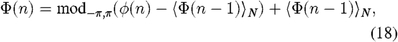
where
2.2. Bias Correction for Power Estimation
Squared visibility estimates from the fringe quadratures require correction for biases attributable to photon noise and detector read noise (F99; Perrin & Ridgway 2005). However, after dewarping the phasors to correct for mismatched stroke versus wavelength, there remain cross terms that make the NUM bias phase dependent. We extend the analysis in F99 for this case, below.
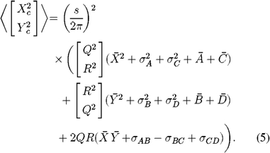
The expectations on the squares of the corrected quadratures Xc and Yc can be written
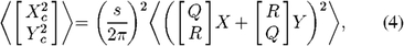
or
The photon-noise variances per bin are shown as  , etc., and the read-noise variances per bin as
  , etc., each with value equal to the correlated-double-sampling (CDS) read variance
  . With an integrating detector, as assumed here, adjacent bins are correlated, viz. σAB ≠ 0, etc., as adjacent bins share a common raw detector read.
The only signal-dependent biases in equation (5) are from photon-noise terms. The read-noise biases calibrate simply from the dark values of  and
and  after correction for detector offsets: call this sum E. Thus the total signal-dependent bias on NUM is 2GN, where
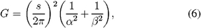
so that an unbiased NUM estimator when using dewarped phasors is given by

where k is the pixel gain in dn per electron. In terms of dewarped quantities only, we substitute N = Nc + πγ(Yc - Xc)/(2s), yielding

If s = 2π, then G = 1/2 and γ = 0, and this expression reduces to the standard result (see F99, eqs. [9]–[11])

2.3. Sliding-Window Estimation
For an interferometer observing through atmospheric turbulence with coherence diameter r0 and wind speed W, the phase-difference coherence time (τ02 = 0.207r0/W) is 4 times smaller than the variance coherence time (T02 = 0.815r0/W) (see P99). In order to maintain adequate continuity between phase samples to allow for unwrapping, we typically require the spacing between samples δt to be ≲τ02. Similarly, in order to avoid excess fringe blurring during the integration time, we typically require the frame time T to be ≲T02. For a typical "full-frame" ABCD implementation, the period of the path length modulation stroke is equal to the frame time, and one phasor estimate is provided per frame. Thus, δt = T, and the frame time is typically limited by the smaller τ02 constraint on continuity, which impacts instrument sensitivity.
The ABCD implementation also affects the performance of the system when the phase estimates are used in a feedforward system to stabilize a second optical path. As discussed in § 5, the error rejection for a feedforward system depends strongly on the total control latency Δ, which includes contributions from the fringe measurement, delay-line bandwidth, and data processing. The component of the control latency attributable to the fringe measurement has two components: (a) the data age, i.e., the average delay between when a photon is detected and when a phasor is computed; and (b) the average sampling delay, equal to one-half of the sampling period. Thus the fringe-measurement latency for a full-frame implementation is approximately the frame time: Δf ≃ T.
However, for the same frame time, it is possible to reduce the spacing between samples, as well as to reduce the control latency, by updating the phasor estimate as individual detector reads become available, rather than waiting for a full frame's worth of data. For example, when detector read c is available, a new value of the bin count C = c - b can be computed. Then using bin counts A and B from the current frame, and D from the previous frame, an updated phasor estimate can be computed using the new information. This approach, sliding-window estimation, is possible with a sawtooth path length modulation stroke, and is implemented on KI.
The KI fringe tracker servo runs at 5 times the frame rate, processing each of the 5 detector reads as they become available. Assume for simplicity an ideal 80% duty cycle path length modulation stroke as illustrated in Figure 1. In this example, at the time of the c read at t = 0.6T, a phasor estimate can be computed from the A, B, C, and D bins centered at 0.1T, 0.3T, 0.5T, and -0.3T, yielding an effective data age of 0.45T. A similar computation for all five reads {z,a,b,c,d} yields data ages of {0.6,0.55,0.5,0.45,0.4}T. Note that at the time of the z read, no new information is available, and the data age is just 0.2T longer than at the time of the d read. Adding the average 0.1T sampling delay of one half of the sample period, the fringe-measurement latency for the five reads is {0.7,0.65,0.6,0.55,0.5}T, with an average value Δf = 0.6T. By comparison, for a full frame readout (at the time of the d read) for this same 80% duty cycle example, the fringe-measurement latency is equal to the data age 0.4T plus the sampling delay of 0.5T, yielding Δf = 0.9T.
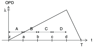
Fig. 1.— Example path length modulation stroke and bin timing for sliding-window fringe measurement. The bin counts are computed from the difference of detector reads as A = a - z, etc. The array is reset after the d read during the retrace of the stroke.
In practice, both the sliding-window and full-frame values will be slightly larger when the actual duty cycle and camera readout time are included. We measured the latency at KI from the phase delay between time-tagged fringe-phase measurements and time-tagged delay-line position measurements for a 10 Hz sinusoidal disturbance. The measured value for the sliding-window implementation is 2.6 ms for a T = 4 ms frame time; this is ∼1.2 ms less than a comparable full-frame implementation would achieve.
We complete this section by returning to the issue of phase unwrapping. With the sliding-window implementation, samples are available at 5 times the frame rate, but we need to account for the different data ages between adjacent samples. Continuing the example in Figure 1, the effective delay from the previous sample for reads {z,a,b,c,d} is {0,0.25,0.25,0.25,0.25}T, with a maximum δt = 0.25T. This is a factor of ∼4 smaller than for the full-frame approach. This maximum value should also be closely achieved in practice, as additional overheads apply to each sample, affecting mostly the overall latency, and not the sample-to-sample spacing.
Thus, with a sliding-window implementation, longer frame times for improved sensitivity can be used while still maintaining adequate phase continuity for unwrapping; or for a fixed frame time, improved unwrapping and feedforward performance can be achieved. For cophasing, KI uses sliding-window estimation with a 4 ms frame time and an update rate of 1250 Hz. For noncophased K-band science measurements, typical frame times are 5 and 10 ms, with update rates of 1000 and 500 Hz, resp.
2.4. Phasor Estimators to Reject Scintillation
The fringe power NUM, as computed from the sum of the squares of the fringe quadratures (and in the absence of full-rate photometric monitoring), is biased by scintillation as the frequency of the scintillation approaches that of the path length modulation stroke. At KI, ordinary atmospheric scintillation is usually quite small, because of the near-infrared wavelength and the aperture averaging of the 10 m Keck telescopes. Most of the observed scintillation is caused by fluctuations of the coupling into the fringe tracker single-mode fibers caused by angular vibrations, guiding errors, and Strehl fluctuations.
KI implements a multistate fringe-acquisition algorithm, similar to that used at PTI, using filtered and unfiltered versions of the fringe S/N squared

to transition among states: thus, high levels of scintillation can cause false transitions. Some amelioration is provided by (S/N)2 thresholds that include a fixed term along with a flux-dependent term that sets a lower limit on V2. However, it is desirable to keep the coefficient of the flux-dependent term as small as possible to allow tracking of extended objects.
To reduce the effect of scintillation bias, the real-time system at KI uses an alternative phasor estimator to compute NUM to estimate (S/N)2 using equation (10) for determining mode transitions. We now compare the scintillation properties of the standard phasor estimator and two alternatives.
2.4.1. Standard Phasor Estimator
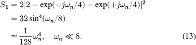
With the standard phasor estimator, as described in § 2.1, the scintillation bias in the fringe power NUM = NUM0 arises because the quadrature estimates X = A - C and Y = B - D are essentially derivatives of the incoming flux I(t), i.e., for a stroke period T, X(t) ∼ I(t) - I(t - T/2) and Y(t) ∼ I(t - T/4) - I(t - 3T/4). For this discussion, we assume a full-frame phasor estimator with a 100% duty cycle, and neglect for now the integration over the bin duration T/4. Thus, in the frequency domain, X(ω) ∼ [1 - exp(-jωT/2)]I(ω), and for unit scintillation at normalized frequency ωn = 2πfscint T, the bias on NUM0 is given by
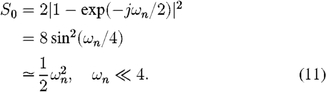
This has an intuitive form, with the bias from scintillation increasing quadratically as the scintillation frequency increases.
For comparison with next two estimators, the read-noise bias on NUM0 is just the last term of equation (9) (assume pixel gain k = 1):

For the standard phasor estimator, the standard deviation of NUM in the read-noise limit is just E0 (see F99). Thus, we use the read-noise bias on NUM as a proxy for the noise on the (S/N)2 estimator.
2.4.2. Modified Phasor Estimator 1
We can create quadrature estimates that are less sensitive to scintillation by subtracting out a local trend from adjacent bins, i.e., we can compute X1 = 2[(B + D)/2 - C] and Y1 = 2[B - (A + C)/2]. With respect to scintillation, these look like centered derivatives, and thus reject low-frequency terms. The bias for unit scintillation on the fringe power estimate  computed from these quadratures is given by
Compared with the standard NUM estimator, the scintillation bias dependence with frequency is now to the fourth power, and the bias drops rapidly with frequency below the corner frequency ωn = 8.
However, this improved rejection comes at the expense of read-noise bias. With nondestructive reads, adjacent bins are correlated. Writing NUM1 in terms of detector reads yields NUM1 = (-a + 3b - 3c + d)2 + (z - 3a + 3b - c)2. The reset noise drops out in this expression, so that the effective noise variance per detector read is 1/2 of the CDS value, and the bias on NUM1 is given by

Because of its ease of computation—it just needs one frame's worth of bin data—and its scintillation-rejection properties, this algorithm was used on KI for the first several years in the computation of (S/N)2 for mode transitions.
2.4.3. Modified Phasor Estimator 2
An alternative NUM estimator can be created which retains the  scintillation rejection of previous version, but with a slightly larger leading coefficient on the bias expression. This estimator uses data from adjacent frames to compute the necessary fringe quadratures. Thus for each new bin count A, B, C, and D, we compute a flux trend by comparison with the prior value of that bin, i.e., on a new A, we compute I' = A - Alast, etc. Thus, in the sliding-window computations, we update the total flux N using the sum of the four most recent bin counts, and update the quadrature estimates for each bin as
On a new A, X2 = A - C - α(A - Alast)/2;
On a new B, Y2 = B - D - α(B - Blast)/2;
On a new C, X2 = A - C - α(C - Clast)/2;
On a new D, Y2 = B - D - α(D - Dlast)/2.
The factor of 1/2 converts the trend measured over 4 bins to the value for a 2 bin difference, and the factor α is for duty cycle correction; with 100% duty cycle (integration time/frame time), α = 1; more typically, α = 0.8–0.9. The bias, for unit scintillation, for a fringe power estimate  computed using these phasor estimates (assuming α = 1) is
While not quite as effective at rejecting scintillation as the previous estimator, this NUM estimator does retain the fourth power dependence with frequency, and has much lower noise. On a new D, NUM2 = (A - (C + Clast)/2)2 + (B - (D + Dlast)/2)2, and thus

which is even smaller than for the standard estimator because of the effective averaging of C and D. The tradeoff for low noise is that the effective frame time is slightly longer than the standard estimator. We find that this NUM estimator works well, and after bias correction using equation (8), is our default in the real-time system for estimating (S/N)2 using equation (10). However, all other phasor computations use the standard estimator.
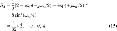
The scintillation bias, for unit scintillation, of the three NUM estimators discussed in this section is plotted in Figure 2. The plot also includes the common factor of sinc2(πfscint T/4) to account for integration over the bin duration T/4.
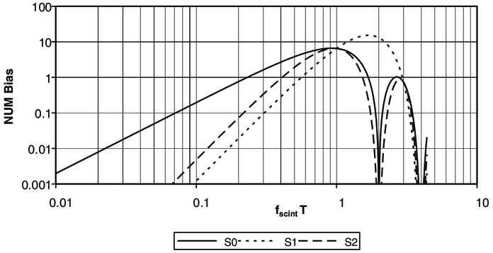
Fig. 2.— Scintillation bias vs. normalized frequency for the three NUM estimators. The standard estimator, S0, has a low frequency dependence of f2, while the scintillation-invariant estimators S1 and S2 have frequency dependencies of f4, and thus reject low to midfrequency scintillation better.
3. FRINGE TRACKING
3.1. Phase and Group Delay Measurement
The KI fringe tracker uses two post-combination single-mode fibers on the two outputs of the Michelson beamsplitter to feed an infrared camera,7 and the camera is typically configured to provide a white-light channel on one output and a spectrometer channel on the other (Vasisht et al. 2003). The white-light channel is typically used for phase estimation for high bandwidth fringe tracking, while the spectrometer channel is used for group delay estimation for central fringe identification. This approach for phase and group delay measurement is similar to that used at PTI.
At KI, we use the sliding-window estimator described in § 2.3 to provide sets of dark-corrected bin counts A, B, C, and D for the white-light pixel and each spectrometer pixel. With the sliding-window estimator, the computations are done at 5 times the frame rate.
For the low spectral resolution modes, we can improve the S/N for phase estimation by combining the white-light and spectral channels to create a synthetic white-light channel. We can create a set of synthetic white-light bin counts by summing the spectrometer bin counts and combining with the white-light bin counts as8
From either the white-light or synthetic white-light bin counts, we compute the complex phasor ΓWL(n) = XWL(n) + jYWL(n), dewarp, and compute the phase as ϕ(n) = arg[ΓWL(n)], as in § 2.1. The raw phase is unwrapped using a first-difference continuity unwrapper with a small amount of memory, viz.
where mod -w/2,w/2(x) is the modulo of x over [-w/2,w/2) and 〈f(n)〉N is an N-point boxcar low-pass filter. Typically N = 2 for this unwrapper. The phase delay x(n) is just Φ(n)λ/2π.9
We compute the group delay g(n) using the spectrometer phasors Γ(n; k) as a function of wavenumber k. To improve S/N, the spectrometer phasors are phase referenced to the WL phase and averaged as

Typically M = 60, or 50 ms for the nuller configuration. The group delay g(n) is then computed from the Fourier transform vs. wavenumber of the average, phase-referenced spectrometer phasor array (see P99). The DFT is zero padded by typically 8 times to avoid scalloping losses, and a quadratic interpolation about the peak is done to improve the group delay estimate.
KI implements different fringe tracker servos for V2 and nulling. The purpose of the tracker is not only to center the phase track point near the peak of the coherence envelope, but also to correct for fringe hops in the continuity unwrapper.
3.2. Fringe Tracking with Continuous Centering
The servo implementation for V2 observations uses a fast inner loop and a slow outer loop, as illustrated in Figure 3, to generate servo targets cK for the fast delay line. The inner loop uses the phase delay x with an integral gain a1; a limiter preceding the integrator constrains the maximum slew rate to prevent fringe blurring. Additional vibration rejection is provided by control block Hn, which will be discussed in § 3.4.10 We typically use an integral gain a1 = 0.1, which provides, for a 5 ms frame time, a 16 Hz closed-loop bandwidth. It is worth noting that for V2 measurements, only the motion during a frame time reduces the fringe visibility, and thus high bandwidth is not required: bandwidth is only required to stay within the coherence length of the channel used for the V2 measurement.
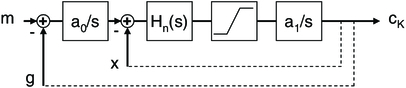
Fig. 3.— Continuous-centering controller; x and g are the estimated phase and group delay, cK is the command to the fringe tracker's fast delay line, and m is a group delay target modulation input. The dotted lines illustrate the logical servo control flow. This controller uses an inner phase loop and an outer group delay loop. The inner loop uses phase feedback and a forward path consisting of an integrator a1/s; a limiter preceding the integrator that clips large errors to prevent fast fringe motion which could cause fringe blurring; and a vibration-control block Hn(s), which we discuss in § 3.4; for now it can be considered a pass-through. The outer loop uses group delay feedback and an integrator a0/s to provide a target to the inner loop. The outer-loop bandwidth is typically 1/10 of the inner-loop bandwidth, so that the loops can be analyzed mostly independently, e.g., for analysis of the outer loop, the inner loop can be replaced by its closed-loop response, which is unity at low frequencies. In steady state, the overall controller servos to zero the group delay, and the integral gain in the outer loop corrects for unwrapping errors in the phase delay estimate x (as well as dispersion differences between g and x). For visibility measurements, the target modulation m slowly varies the track point over one wavelength in order to average out phase-dependent systematics.
The outer loop uses the group delay g with an integral gain a0; typically a0 ∼ a1/10, providing an outer loop bandwidth of 1/10 of the inner loop, typically 1.6 Hz for a 5 ms frame time at KI. The outer loop implements the fringe centering, by providing the target for the phase-tracking inner loop. Thus the outer loop corrects for the arbitrary zero point of the unwrapped phase, as well as for fringe hops which may occur in the continuity unwrapper. The correction occurs slowly, at the time constant of the outer loop, so there is insignificant fringe blurring from the changing phase target. By centering continuously, rather than stepwise, no synchronization or coordination of centering commands is needed, and this simplification is one of the advantages of this implementation.
The outer loop also accepts an external target. For V2 measurements, we typically introduce a triangular group delay target modulation, m, with a one-wave peak-to-peak amplitude and a period of 5 s; the period is chosen to be short compared with the length of a science scan. The effect of the target modulation is that the average V2 for the scan includes measurements over a near-uniform distribution of phases. This greatly reduces the effect of errors that are periodic with a wavelength, such as those that are attributable to errors in the assumed wavelength, or residual nonlinearities in the path length modulation stroke.
It is important to note that while phase delay and group delay are shown as logically equivalent in Figure 3, they differ in practice due to systematic and random dispersion. The systematic dispersion is attributable to average air and material dispersion, with a sidereal component from changing air paths as the delay lines move. The random dispersion is primarily attributable to water vapor seeing (see Colavita et al. 2004a). In the inner-loop/outer-loop implementation, the dispersion gets pushed into the phase target. As this is a low-bandwidth effect, it is not especially important for V2. In fact, for V2, it is the proper behavior, as we wish to track to the center of the coherence envelope, including the effects of dispersion, in order to maximize V2.
3.3. Fringe Tracking with Discrete Centering
For phase referencing, as implemented for the KI nuller, we wish to track to constant phase, rather than to constant group delay, as in the previous V2 implementation. The implementation we use for phase referencing is shown in Figure 4. In the figure, the inner loop, using the phase delay, remains unchanged from Figure 3. What does change is the source of the phase target, which was previously a continuous target from an outer-loop group delay servo, and included dispersion as well as integer fringe hops. In Figure 4, the phase target is now always an integer number of wavelengths, so we always track to "zero" phase. In principle, we could implement this simply, adding or subtracting wavelengths to the phase target to keep the group delay within ± 0.5λ. However, with varying dispersion, especially from water vapor seeing, the phase target would continually toggle. For phase referencing, at least for reasonably short tracks where the change in the systematic dispersion due to sidereal motion is less than a wavelength, it is better to follow a single phase point as it wanders within the coherence envelope. For longer tracks, it is necessary to periodically reset the track point in order to not drift too far from the center of the envelope.11
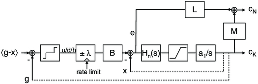
Fig. 4.— Discrete-centering controller; x and g are the estimated phase and group delay, cK is the command to the fringe tracker's fast delay line, and 〈g - x〉 is a low-bandwidth, nonwrapping estimate of the dispersion. The inner phase loop for this controller is identical to that in Fig. 3. However, the outer loop for this controller generates a target for the inner loop which is constrained to be an integer number of fringe hops. If the dispersion is zero, the outer loop just compares the group delay against a threshold, typically ± 0.75λ. If the threshold is exceeded, the outer loop steps the target to the inner loop by one wavelength. The low-pass filter B smooths the change in the target to prevent fringe blurring; the time between steps is limited to ensure that previous fringe hops are fully reflected in the group delay before making another hop. Because of dispersion, even in the absence of unwrapping errors, g ≠ x, and thus we use as a target for the outer loop a low-bandwidth dispersion estimate 〈g - x〉. This has the effect that the servo follows a fixed phase point on the fringe, even as that point moves within the fringe envelope because of changing dispersion. At the top of the figure is shown the generation of the feedforward command, cN, to the nuller's fast delay line, computed from the sum of the K-band command, cK, filtered by block M, and inner-loop error, e, filtered by block L.
Thus, in Figure 4, we compare the group delay with a slow, nonwrapping average of the dispersion 〈g - x〉; we describe how this is computed in § 4. A comparator, with thresholds of typically ± 0.75λ, increments or decrements a counter in units of λ. The output of this counter passes though a short boxcar filter, B, which limits the slew rate of the step, and then to the input of the phase loop; typically B is 20 samples long. The rate at which the wavelength counter can change is limited to allow fringe hops to be fully reflected in the group delay, including the time it takes to fill the group delay coherent average filter, before another hop can occur. Typically, the limit is 100 samples between hops.
3.4. Active Vibration Cancellation
With typical closed-loop bandwidths of 16 Hz, the basic fringe tracker has limited ability to attenuate high frequency disturbances. However, at KI there are residual disturbances at high frequencies that are not observed by the laser metrology or accelerometers. Most of these disturbances are narrowband vibrations, and typical sources are induction motors which introduce vibrations at ∼29 and ∼58 Hz (for US 60 Hz ac power), as well as "mystery" sources at other frequencies. For such narrowband disturbances, it is possible to actively suppress them to improve fringe tracker performance, even though their frequencies exceed the ordinary fringe servo closed-loop bandwidth.
The control block used for vibration suppression is shown in Figure 5, and implements higher harmonic control (HHC; Shaw & Albion 1981). This block is inserted in the fringe tracker forward path as shown in Figures 3 and 4, and provides loop gain at the frequency of the vibrations. As shown in Figure 5, the overall control block has a pass-through path on the bottom, and multiple HHC blocks for each vibration frequency under control. While each control block typically controls five frequencies at KI, we will generally assume a single controlled frequency for the rest of this discussion.
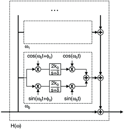
Fig. 5.— Active vibration-control block, showing one of several HHC controllers, and the pass-through path on the bottom. The HHC controller in the figure is tuned to frequency ω0: it mixes the frequency band near ω0 to baseband, applies an integral controller, and then mixes it back up to the original frequency. This provides gain over a narrow frequency range which is used in the inner servo loops of Figs. 3 and 4 to suppress narrowband disturbances.
In Figure 5, quadrature oscillators configured to the nominal vibration frequency mix the input signal to baseband. The phase shift ϕ0 on the input oscillators compensates for phase shifts in the forward path of the fringe tracker at the frequency of the vibration, including the phase of the ordinary fringe tracker integral controller. The controllers on the baseband disturbance signals are implemented as leaky integrators with gain k0. The small leak δ is so that the oscillators decay to zero when the fringe tracker enters a hold state on loss of lock, although it does limit the ultimate vibration rejection. The integrator outputs are then mixed back up to the original frequency and summed with the pass-through signal.
The response of the HHC controller is given by Hall & Wereley (1989; summarized in Sievers & Von Flotow 1992). Including the pass-through, and the finite leak in the HHC integrator, the transfer function of the vibration control block is
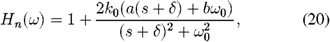
where a = cos ϕ and b = sin ϕ. Thus, Hn(ω) provides high gain at the configured frequency, and is approximately unity elsewhere.
At KI, Hn(ω) is used in series with an ordinary servo controller G(ω). While the approach is generalizable, we are normally interested in providing suppression above the unity-gain frequency of the ordinary servo, i.e., where G = |G(ω0)| ≪ 1; we assume G incorporates any dynamics of the plant. In this case, near the configured frequency, the second term of equation (20) is ≫1, and so we can approximate Hn(ω) near ω0 as
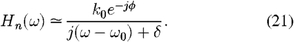
In our application, we typically set ϕ ≃ arg[(G(ω0)]. The 3 dB half width of these active notches Δω, for Δω≫δ, depends on the product of the HHC gain and the ordinary loop gain as Δω ≃ Gk0 rad/s, with peak suppression ≃Δω/δ.
To first order, the maximum notch width is limited by the requirement that the ordinary controller and plant be approximately constant in phase and amplitude over the notch width in order to control the phase at the loop crossovers on either side of the notch. This constraint is similar to that which limits the bandwidth of the ordinary controller, and thus the notch widths are typically limited to a fraction of the ordinary closed-loop bandwidth.
We find these modules to be robust and effective in suppressing vibrations with well-known frequencies, which is the case for the largest-amplitude vibrations at KI.12 The HHC approach also allows for accurate single-parameter tuning of the notch frequency. For a different approach to narrowband suppression, see Di Lieto et al. (2008), which describes the adaptive algorithm used on VLTI's FINITO fringe tracker.
As the ordinary controller gain, while less than unity at the frequencies where these notches are employed, is still finite, and there are multiple notches which can interact, we usually tune the notches empirically. In our implementation, we include a test oscillator in the HHC block to measure arg[(G(ω0)], and we set the notch gain based on frequency-response measurements in order to balance notch depth with band-edge peaking. Typically bandwidths of order 1 Hz are used, which allows for some uncertainty in the vibration frequency, e.g., to account for shifts in the frequency of induction motors with changing loads. For example, with a 1 Hz notch width, and δ ≪ 1 Hz, a factor of ∼4 suppression is possible for uncertainties in the vibration frequency of ± 0.125 Hz.
4. DISPERSION ESTIMATION
One of the modes of KI is broadband nulling at 10 μm (see Colavita et al. 2009 and references therein). Because of the integration times required to obtain adequate S/N, high bandwidth path length control to correct for rapid atmospheric turbulence is not possible using just the 10 μm light, and thus the high bandwidth control is provided by the fringe trackers using the K-band light. Because of atmospheric dispersion, simple achromatic feedforward is not adequate when high accuracies are required, and a correction for the effects of atmospheric water vapor is also required (Colavita et al. 2004a; Colavita 2010). The path length fluctuations attributable to water vapor can be estimated from the relative group delay, and can be used with a dispersion model to correct the N-band path length residual attributable to water vapor. In principle, the relative group delay is just the difference of the group delay g and the phase delay x described in § 2.1. In practice, the phase delay x is subject to unwrapping errors, caused by, e.g., fast fringe motion or signal dropouts, and a more robust estimator is desired, especially for low S/N conditions. The algorithm used at KI takes advantage of the fact that the water vapor coherence time is much longer than the dry air coherence time.
We start by averaging the phase delay x with a filter that has the same length as the group delay coherent averaging filter in equation (19): call this value x', so that x' has the same latency and smoothing as g, and compute Λ = g - x'. If there were no unwrapping errors, Λ would have a Gaussian-like distribution about its true value, and we could simply average Λ to improve its S/N. However, if the true value of Λ is changing slowly over the desired averaging times, we can average the central modulo in order to be robust against unwrapping errors in x. Because of the width of the distribution, which can exceed one wavelength under low S/N conditions, we need to choose the offset about which to do the central modulo to center the distribution in the interval. In this case, the average of the wrapped quantity will suffer the least bias from the tails of the distribution. As an extreme example of the type of bias that can arise, assume that the true value of Λ is slightly less than λ/2. If we do a central modulo about zero, the wrapped distribution will be peaked near ± λ/2, and a simple average will yield a value near zero, instead of the true value.
A simple algorithm for selection of the offset about which to do the central modulo is to choose the one that minimizes the mean square of the distribution, and this is what we implement. There are certainly other approaches that could be used, but this is computationally efficient in our system. Thus, for each time sample, for a set of offsets {pi}, typically {-0.5,-0.375,-0.25,...,0.375}λ, we compute the differences {δi = mod -λ/2,λ/2(g - x' - pi)}, averages {di = 〈δi〉+pi}, and mean squares  . Typical averaging times are 1.0 s. If c is the index of the offset that gives the minimum value of si, our estimate of the average dispersion is just dc. In practice, we do some (probably unnecessary) interpolation, and compute a three-point quadratic fit to the mean square about offset pc to determine an "optimal" offset, and then interpolate between the nearest di to determine dc. As dc is a wrapped quantity, we run it through a first-difference continuity unwrapper with a small amount of memory (typically 1 s) to yield our final dispersion estimate
  .
.
This value is used to compute the nuller water-vapor feedforward quantities (Colavita 2010), and to provide the zero point for the outer loop for the cophasing (discrete-centering) fringe tracker in Figure 4. Strictly, the zero point of  is somewhat arbitrary. However, changes from this zero point are correctly measured, and this is all that the nuller requires, as the nuller is subject to a number of different zero point offsets, which it determines at low bandwidth directly from the 10 μm fringe signal. In particular, for control of the nuller's longitudinal atmospheric dispersion corrector,
  is high pass filtered at 0.002 Hz, and we rely upon direct 10 μm feedback to control the very low frequencies.
5. FEEDFORWARD CONTROL
As discussed previously, one role of the K-band fringe trackers is to provide (coaxial) phase referencing, or cophasing, for the nuller. To first order, as the nuller and fringe tracker have separate delay lines, one could just slave the nuller delay lines to the K band delay lines. However, as the nuller delay lines are outside of the fringe tracker feedback loop, the K-band fringe tracker error can be used in addition to the K-band feedback signal to generate commands to the nuller delay lines to improve the cophasing performance without violating stability criteria (Lane & Colavita 2003).
The implementation at KI is shown schematically at the top of Figure 4, where cK is the command to the K-band delay lines from the discrete controller and e is the K-band fringe servo error. These two inputs are filtered by blocks M and L, and summed to generate the command to the nuller delay lines, cN. To first order, blocks M and L are just pass-throughs, e.g., M = L = 1; in practice, they can be used optimize performance, and in our implementation L is a lead filter, and M is a short boxcar filter.
A simple controls model of the feedback and feedforward systems is given in Figure 6, where d is the disturbance input, eFB is the feedback error (seen by K band), and eFF is the feedforward error (seen by N band). In the figure, block D models: the overall system time delay, Δ, including the fringe tracker measurement latency Δf as discussed in § 2.3; the delay line command response; and compute and transport delays. Block D also includes the amplitude effect of the finite fringe tracker frame time T, viz.

Block G models the feedback controller; typically G is just an integrator: G(f) = a/(j2πf). With these definitions, the feedback error response takes the usual form
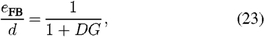
which at low frequencies with integral control has the asymptotic form
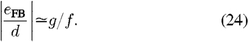
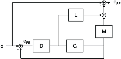
Fig. 6.— Servo performance model. Blocks D and G model the forward path of the feedback controller, and eFB is the feedback error in response to disturbance d. The feedforward command is computed as in Figure 4 from the feedback-loop output and error filtered by blocks M and L. The feedforward error, eFF, is the difference of disturbance and the feedforward command. This model is used for the performance analyses in the text.
Blocks M and L in Figure 6 are the same as in Figure 4, where M filters the K-band delay line command, and L filters the fringe tracker error. The feedforward error response for this system can be written
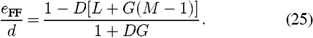
In this expression, if the gain G = 0, or else M is chosen to compensate for the time delay, viz. M = LD, then
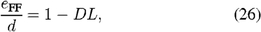
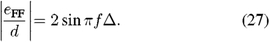
independent of the feedback gain. In this case, if L = 1, and neglecting the amplitude effect of the sinc function in equation (22), this becomes a time-delay–limited response, and the response as a function of frequency f is given by
If instead M = 1, then
and the feedforward error response is the product of the time-delay–limited response (eq. [26]) and the feedback response (eq. [23]). In this case, the low frequency-error response falls off as frequency squared for an integral feedback controller. This behavior is desirable to provide good cophasing performance in the presence of the steep atmospheric power spectrum.
As noted previously, blocks L and M can be used to improve performance. For block L, we usually implement a lead filter, which can compensate some of the system latency at low frequencies, in exchange for some peaking at higher frequencies (but where the response is attenuated by the low pass filtering of the finite frame integration time included in equation [22]). For block M, we usually introduce a small amount of delay, ΔM, implemented as a short boxcar filter (the amplitude response is not significant over the frequency range of interest). This delay reduces some midfrequency peaking attributable to the interaction of the numerator and denominator in equation (28), but limits the ultimate low frequency rejection. This can be seen by letting G → ∞ in equation (25): the low frequency error response becomes time-delay–limited as 1-M, with error response given by equation (27) with Δ = ΔM.
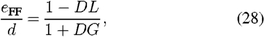
Figures 7 and 8 show model and measured performance for the cophasing system at KI. The measurements were made by introducing synchronized disturbance targets on the K- and N-band delay lines, and measuring the residuals when the fringe tracker was tracking an internal source. All data is for a frame rate of T = 4 ms, and a sample rate of 1250 Hz for our 5 point sliding-window implementation. Control blocks G, L, and M were implemented as:
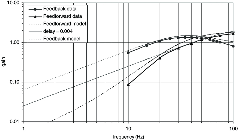
Fig. 7.— Model feedback and feedforward error response and measured data; a 4 ms time-delay-limited response is included for reference. The error response with feedforward is better than with feedback below ∼60 Hz.
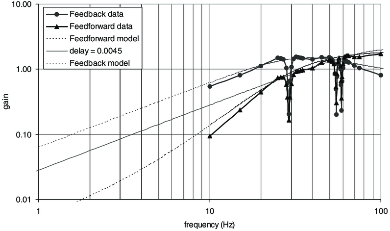
Fig. 8.— Model feedback and feedforward error response and measured data with 3 notches enabled; a 4.5 ms time-delay-limited response is included for reference. The broadband performance is similar to Fig. 7, but with slightly more high-frequency latency. The notches provides addition rejection at selected frequencies.
Feedback controller G: Integral controller with a 15.9 Hz crossover (dimensionless gain 0.08);
Error filter L: Lead filter with a zero at 133 Hz (and an implicit pole at the 625 Hz Nyquist frequency; at low frequencies, this filter looks like a 1 ms time lead);
Feedback filter M: Time delay with ΔM = 0.8 ms (implemented as a nonbuffered 3-point boxcar filter).
For the system delay in block D in the model, we used Δ = 4.0 ms, consisting of 2.6 ms for the fringe measurement, discussed in § 2.3, 0.7 ms for the measured delay line command response, and 0.7 ms for compute and transport delays.13
Figure 7 shows the measured feedback and feedforward responses versus the models: the compliance is fairly good. The feedforward performance is better than the feedback performance below about 60 Hz, with the error decreasing rapidly with decreasing frequency until the limit imposed by the delay ΔM comes in. At this point, the error rejection continues to improve, but only linearly with decreasing frequency. In the critical 30–60 Hz region, the feedforward response can be modeled as a simple 4 ms time delay. At lower frequencies, the performance is substantially better than a simple time delay due to the contribution of the feedback component. The parameters used here of course represent a compromise: with a lower value of the integral gain, or a larger compensating delay ΔM, the feedforward response would approach a delay-limited system with a time delay of approximately 3 ms. The larger effective midfrequency time delay in our implementation is in exchange for improved low frequency rejection and maintenance of good feedback performance.
Figure 8 is like Figure 7, except now with three active notches enabled, as described in § 3.4. The notches add a small amount of out-of-band phase, and we empirically increase the system delay in the model by 0.5 ms to account for this effect. In the 30–60 Hz region, the feedforward response can be modeled as a simple 4.5 ms time delay, but again with improved performance at lower frequencies. The parameters in this implementation are also a compromise: lower values for the notch gains would reduce the out-of-band phase, but would narrow the notch widths, reducing robustness to changes in disturbance frequencies.
The cophasing implementation for the nuller key science program (Colavita et al. 2009) was essentially as described here; the only changes during the program were to the precise notch frequencies. An interesting engineering aspect of the system is that, because of the low nuller measurement bandwidth, the nuller telemetry provides only limited data on the effectiveness of the cophasing on the sky subject to actual disturbances. Thus, we rely on the fringe tracker servo error, and the model given here, to estimate the nuller path length error. So if PFB(f) is the measured feedback error power spectrum from the fringe tracker, we estimate the feedforward error power spectrum for the nuller using equations (23) and (25) as

and the residual feedforward error as
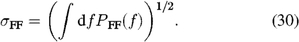
Typically we achieve 150 to 200 nm rms feedforward residuals, with variations attributable to the instantaneous disturbance environment and the external atmosphere. Figure 9 shows nighttime data from one of the nights of the nuller key science run. Chart (a) shows the fringe tracker residual power spectrum, while charts (b) and (c) show the derived power spectrum, and the reverse cumulative power, of the nuller residuals computed from the fringe tracker residual power spectrum using equation (29). For this night, the nuller residuals have approximately equal contributions from frequencies above and below 50 Hz. For comparison, we also plot the power spectrum and reverse cumulative power of the V2 windowed residuals computed from the fringe tracker residual power spectrum and the V2 windowing function 1 - sin c2(πfT). These residuals are smaller than for the nuller, as only fluctuations within the stroke period T cause blurring, whereas the nuller is sensitive to both low and high frequency fluctuations.
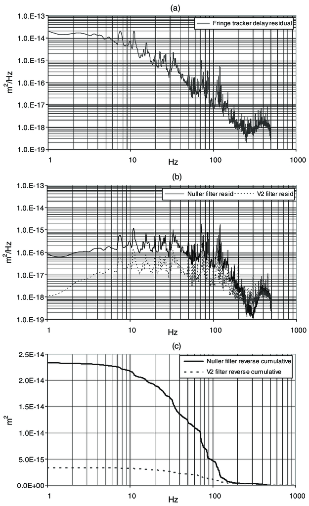
Fig. 9.— These charts shows performance from UT 2008 night 50 at 08:16, a fairly quiet night, which had a fringe tracker jitter (i.e., first-difference [full-frame] rms) of 0.5 μm rms. Chart (a) shows the measured power spectrum of the fringe tracker path length residuals; chart (b) shows the derived power spectra of the residuals for nulling (solid trace) and V2 (dotted trace) measurements; chart (c) shows the reverse cumulative power of the PSDs in (b). The nuller residual power spectrum is computed from the power spectrum in chart (a) using eq. (29). For this night, the nuller residuals have approximately equal contributions from frequencies above and below 50 Hz; the low-frequency asymptote in chart (c) of 2.4 × 10⁻¹⁴ m2 is the integral under the nuller residual power spectrum, for total fluctuations of 155 nm rms. The V2 residual power spectrum is computed as the product of the power spectrum in chart (a) and the V2 filter function 1 - sinc2(πfT), which models the blurring during a 4 ms integration time. As this windowing function rejects low-frequency power, the low-frequency asymptote in chart (c) for V2 is lower, yielding windowed fluctuations of 60 nm rms.
The Keck Interferometer is funded by the National Aeronautics and Space Administration (NASA). Data were obtained at the W. M. Keck Observatory, which is operated as a scientific partnership among the California Institute of Technology, the University of California, and NASA. The Observatory was made possible by the generous financial support of the W. M. Keck Foundation. Part of this work was performed at the Jet Propulsion Laboratory, California Institute of Technology, under contract with NASA.
Footnotes
- 6
- 7
With post-combination fibers, we do not have separate photometric channels—a tradeoff to maximize S/N for phase tracking. For V2 measurements, our standard observing sequence interleaves 5 sets of single-aperture flux measurements during the fringe scan to approximate simultaneous photometry; the ratio of the average of the single-aperture fluxes provides an estimate of the true flux ratio during the scan, and is used to correct the final V2 measurement.
- 8
This form results as we compute the phasors after summing the bins; in terms of phasors, the right-hand side just implements XWL - Xspec, YWL - Yspec, and NWL + Nspec.
- 9
We tend to use boxcar (FIR) filters for implementing low pass filters at KI, rather than simple fading-memory (IIR) filters; this is a useful robustness measure, as data outliers have a finite lifetime in the filter memory. Our implementation at KI uses simple pushes and pulls from a running average to maintain fixed cost, but with a periodic resynchronization to avoid corruption.
- 10
We describe only the lock-mode behavior. The system behavior and control of state during fringe acquisition and on loss of lock is important, but beyond the present scope.
- 11
We readily see this effect for long tracks, manifesting itself as a smooth decrease in white-light V2 with time.
- 12
We have also used them in other subsystems of KI (see Colavita et al. 2004b); the current version is adapted from one originally coded by E. Hovland for tilt control.
- 13
As part of the overall preparations for the nuller mode, the delay line servo was optimized to improve the linearity of the phase of the command response for use in this feedforward application. In addition, a special low-latency control input was added to accept the output of the lead filter L.