
ABSTRACT
The ALMA (Atacama Large Millimeter Array) North American and European prototype antennas have been evaluated by a variety of measurement systems to quantify the major performance specifications. Near‐field holography was used to set the reflector surfaces to 17 μm rms. Pointing and fast‐switching performance was determined with an optical telescope and by millimeter‐wavelength radiometry, yielding 2'' absolute and 0 6 offset pointing accuracies. Path‐length stability was measured to be ≲20 μm over 10 minute time periods using optical measurement devices. Dynamical performance was studied with a set of accelerometers, providing data on wind‐induced tracking errors and structural deformation. Considering all measurements made during this evaluation, both prototype antennas meet the major ALMA antenna performance specifications.
Export citation and abstract BibTeX RIS
1. INTRODUCTION
In the early stages of the collaboration between the National Radio Astronomy Observatory (NRAO) and the European Southern Observatory (ESO) toward the joint design, construction, and operation of a large millimeter array (now called the Atacama Large Millimeter Array, or ALMA, project), it was agreed that each of the partners would acquire from industry a prototype of the planned 12 m diameter antennas. The specifications of these antennas are beyond the current state of the art in accurate reflector antenna technology. Considering that 64 of these antennas would eventually be needed, this step appeared warranted in order to mitigate performance risk and increase competition among prospective manufacturers. It was also agreed that the antennas would be placed next to each other at a suitable site and subjected to an extensive evaluation program to be carried out by a joint team of scientists and engineers drawn from the institutes of the ALMA collaboration.
The two ALMA prototype antennas are located at the site of the Very Large Array (VLA) in New Mexico. This site provides a reasonable compromise between the quality of the atmosphere, necessary for millimeter‐wavelength operation, and ease of construction and operation. The latter is provided by the existing infrastructure of the VLA site. However, the atmospheric characteristics allow operation only at relatively long millimeter wavelengths during the dry winter months. Thus, the antennas have been equipped with evaluation receivers for the wavelength bands near 3 and 1.2 mm.
The evaluation of the antennas has been carried out by the Antenna Evaluation Group (AEG), which consists of experienced "antenna integrators and commissioners" from both the Associated Universities, Incorporated, (AUI)/NRAO and the ESO. The charge of the AEG was to subject both antennas to a series of identical tests that would indicate the compliance (or not) of the antennas with the specifications. The core of the AEG is composed of the authors of this paper.
2. DESCRIPTION OF THE PROTOTYPE ANTENNAS
The ALMA prototype antennas are altitude‐azimuth–mounted Cassegrain reflector systems of 12 m diameter with a reflector surface and pointing accuracy that is suitable for observations in the 0.3 mm submillimeter band. VertexRSI delivered an antenna to AUI/NRAO (see Fig. 1), and ESO obtained an antenna from the Alcatel/European Industrial Engineering (EIE) consortium (AEC; see Fig. 2). The main characteristics of the antennas are summarized in Table 1.
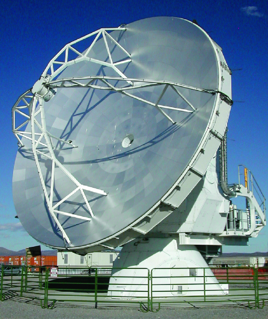
Fig. 1.— VertexRSI ALMA prototype antenna.
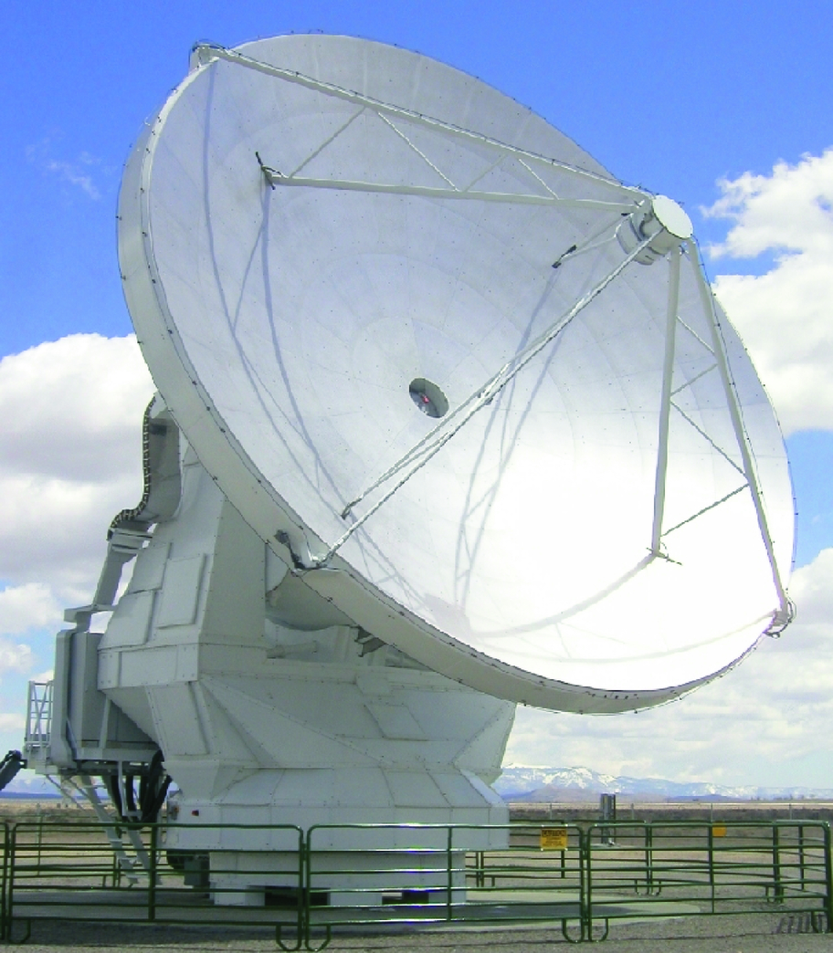
Fig. 2.— AEC ALMA prototype antenna.
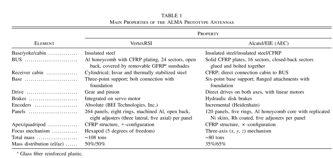 |
The two antennas show interesting differences. To minimize structural deformations due to temperature changes, both make extensive use of carbon fiber reinforced plastic (CFRP) for the backup structure (BUS) of the reflector. The BUS is a box structure, thus avoiding the need to design and fabricate the intricate joints of a space‐frame structure in CFRP. The AEC has realized the entire elevation structure (receiver cabin and connection to BUS) in CFRP, while VertexRSI applies insulated steel for the cabin and Invar for the connection cone to the BUS. For the drive systems, VertexRSI uses a traditional pinion‐and‐gear rack system, while AEC uses a direct linear drive, such as that applied in the VLT (Very Large Telescope) optical telescopes and the Berkeley‐Illinois‐Maryland Association (BIMA) antennas.
There are significant differences in the choice of size and technology of the reflector panels. The VertexRSI antenna has relatively small panels that are made of machined aluminum and have been chemically etched to achieve the required effective scattering of solar heat radiation. They have separate axial (five) and lateral (three) adjustable supports. The AEC panels are of a novel design by Media Lario. Electroformed nickel skins, replicated from a machined steel mold, are bonded to a 20 mm thick aluminum honeycomb core. To improve the thermal behavior under sunlight, the surface is coated with 200 nm of rhodium. These larger panels have five adjustable axial supports, which also provide sufficient stiffness in the lateral direction. Because of the more extensive use of the relatively lightweight CFRP, the AEC antenna is significantly lighter than the VertexRSI antenna.
3. MAJOR SPECIFICATIONS
The ALMA antennas will be used to a shortest wavelength of about 0.3 mm while located at 5000 m altitude in Chile under rather extreme conditions of strong wind and sunshine. Consequently, the requirements on the accuracy and stability of the reflector surface contour and the pointing and tracking behavior are very high. In fact, no radio telescope of comparable size has been designed to the specifications listed below.
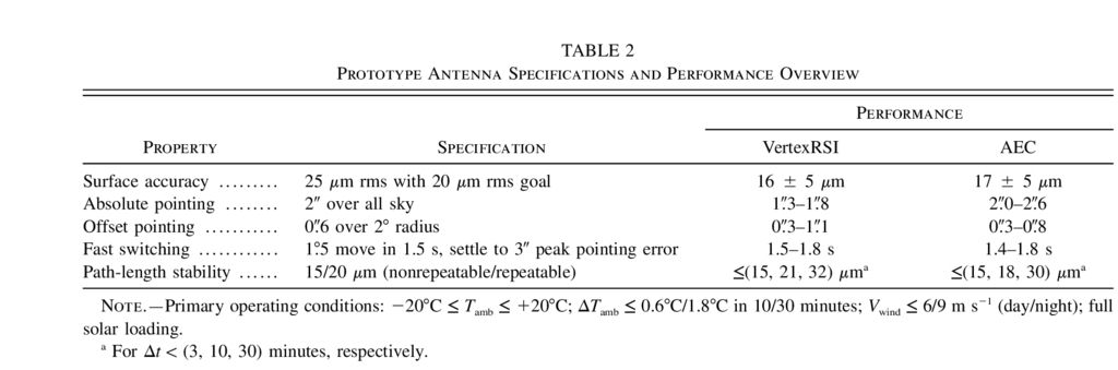
It has been the main task of the AEG to establish the compliance of the ALMA prototype antennas with the major performance specifications (see Table 2). These specifications must be satisfied under all attitude angles of the antenna and all environmental conditions; in particular, wind of 6 m s−1 (day) and 9 m s−1 (night), as well as full solar illumination from changing directions.
 |
Because of the interferometric mode of operation of ALMA, some unusual specifications have been introduced, such as path‐length variations and the capability of very fast switching between two relatively close points on the sky. It is beyond the scope of this paper to elaborate on the reasons for these specifications.
4. EVALUATION RESULTS
The major performance specifications, results, and primary operating conditions during which these specifications apply for the ALMA prototype antennas are listed in Table 2. In the following, we describe how the performance of the ALMA prototype antennas was derived within the context of each performance specification. The technical details that describe the various measurement systems and techniques used to derive these results can be found in J. Mangum et al. (2004, unpublished),2 Baars et al. (2006), Greve & Mangum (2006), M. Holdaway et al. (2004, unpublished),3 Snel et al. (2006), P. Wallace et al. (2004, unpublished),4 J. Mangum & A. Greve (2004, unpublished),5 and J. Mangum (2004, unpublished).6 In the following, we describe the measurements that led to the summary results listed in Table 2.
5. REFLECTOR SURFACE ACCURACY
5.1. Near‐Field Holography Measurements
A near‐field holographic method was used to measure and set the surface to an accuracy of better than 20 μm rms. A transmitter on a 50 m high tower at a distance of 310 m provided the signal at 79 or 104 GHz. See J. Mangum et al. (2004; see footnote 2) and Baars et al. (2006) for further details describing this holographic technique. Figure 3 shows a typical surface error map derived from these holographic measurements.
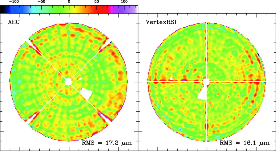
Fig. 3.— Typical final holographic surface map of the AEC (left) and VertexRSI (right) prototype antennas. Note the ×‐shaped (AEC) and +‐shaped (VertexRSI) feed leg structure. The poor measurement results obtained near the feed leg structures of each antenna are due to the difficulties encountered with holographic measurements near these structures.
The holographic measurement and setting of both antennas was performed immediately after the antennas became available for evaluation. During a period of about 1 year, the antennas were subjected to a number of hard loads, such as fast‐switching tests, drive system errors resulting in strong vibrations, and high‐speed emergency stops. In addition, the influence of wind and diurnal temperature variations on the surface stability was a point of concern. It was therefore decided to close the evaluation program with a second holographic measurement of the reflector surfaces. This was done in 2004 December to 2005 February during relatively good atmospheric conditions. It was during these measurements that we discovered that we had not properly taken care of a correction explained in Baars et al. (2006). This correction, which did not affect the final interpretation of the prototype antenna surface accuracy performance, was subsequently applied properly. The final surface maps are shown in Figures 4 and 6. Both antennas were set to a surface accuracy of 16–17 μm rms.
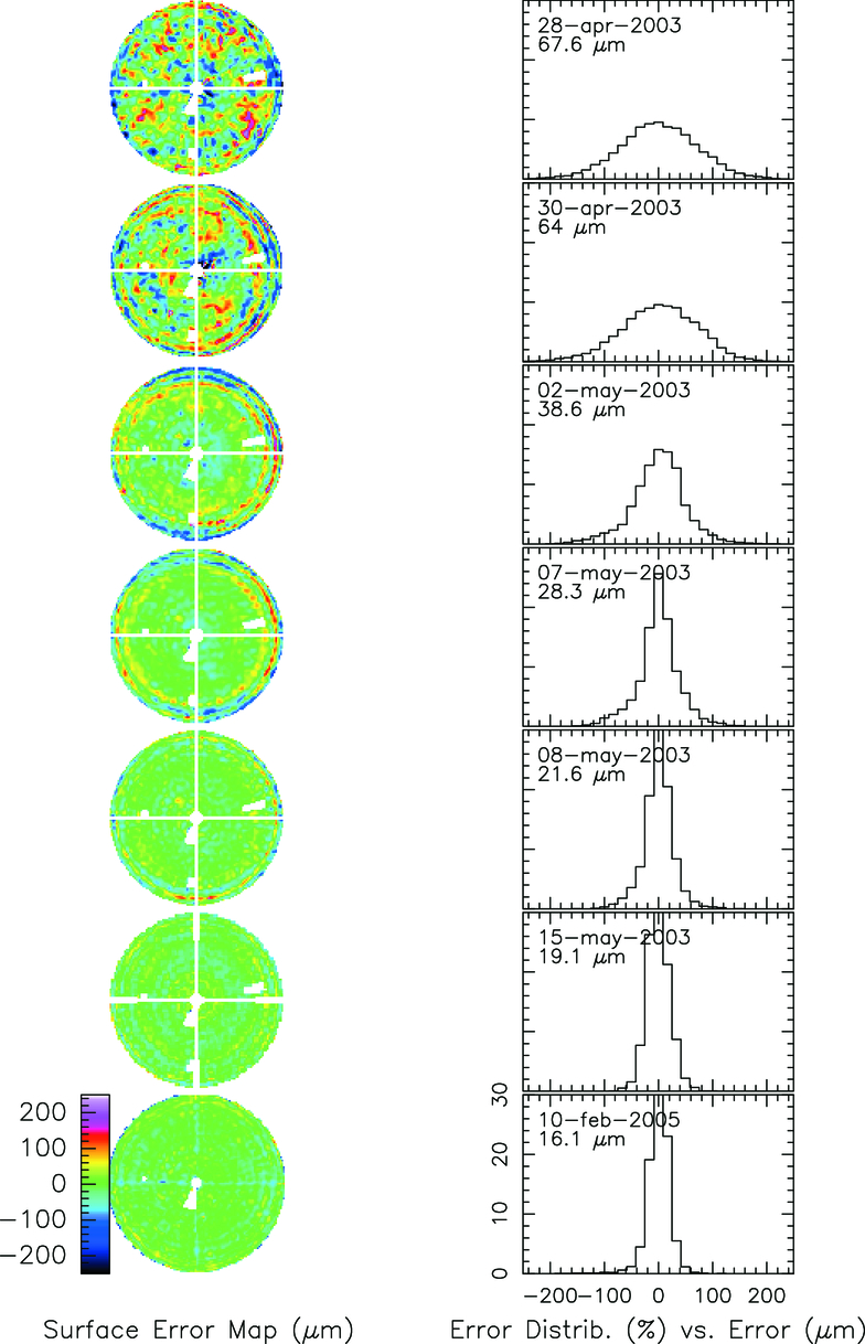
Fig. 4.— Sequence of surface error maps with intermediate panel setting for the VertexRSI antenna. The surface contours are shown on the left side, the error distribution on the right. The white cross and the small white areas represent the quadripod and a few faulty panels, and they were not considered in the calculation of the rms error. Progression to the final surface rms included holography system checkout, so it does not represent the time required to set the VertexRSI antenna to its final surface.
5.1.1. Overview
VertexRSI antenna: The antenna was delivered with a nominal surface error of 80 μm rms, as determined from a photogrammetric measurement. Our first holography map showed an rms of approximately 85 μm. A first setting of the surface resulted in an rms of 64 μm. In four more steps of holographic measurement followed by adjustment, the surface error decreased to 19 μm rms.
The sequence of surface error maps, along with the rms and the error distribution, is shown in Figure 4. As allowed in the specification, we have applied a weighting over the aperture that is proportional to the illumination pattern of the feed. This essentially diminishes the influence of the surface errors in the outer areas of the reflector. The white areas in the surface error maps are the quadripod, the optical pointing telescope, and a few bad panels that could not be set accurately. All of these structures were left out of the calculation of the final overall rms value.
With increasing accuracy, the presence of an artifact in the outer area of the aperture became apparent. There was a wavy structure in the outer section, with a "period" that was too large to be inherent in the panels. Experiments with absorbing material showed that it was not caused by multiple reflections. The effect can be described by a DC offset in the central point of the measured antenna map, i.e., some saturation on the point with the highest intensity. By adjusting this offset in the analysis software, most of the artifact could be removed. This has been done with the final data. The additional set of follow‐up holography measurements in the period of 2004 December to 2005 February did not suffer from this signal saturation, and no artifact was observed in these follow‐up maps. Checks of the holography hardware indeed suggest that the 2003 holography measurements did experience a small amount of signal saturation.
The adjustments were done with a simple tool. Two people on a man‐lift approached the surface from the front, where the adjustment screws are located (see Fig. 5). The time needed for an adjustment of the total of 1320 adjusters was 8 hr, as required by the specification.
The best surface maps were obtained at night. During the spring 2003 period, they consistently show an rms of about 20 μm. Daytime maps tend to be somewhat worse; typical values of the rms lie between 20 and 25 μm. Part of this is certainly due to the atmosphere, even over the short path length of 315 m.
AEC antenna: The apex structure of the AEC antenna does not enable us to mount the holography receiver inside the apex structure cylinder, as is the case for the VertexRSI antenna. Thus, in this case the receiver was bolted to the flange on the outside of the apex structure. Consequently, the feedhorn was brought to the required position by a piece of waveguide of about 500 mm length. This caused significant attenuation in the received signal from the reflector to the mixer. Considering the available transmitter power, we concluded that this would not significantly jeopardize our measurement accuracy.
The AEC antenna surface was set by the contractor with the aid of a Leica laser tracker. The rms of the surface was reported by the contractor to be 38 μm. After this measurement, an accident caused the elevation structure to run onto the hard stops at high speed. The contractor decided to repeat the surface measurement and obtained an rms of 50 μm, with some visible astigmatism in the surface.
Our first holography map indicated an rms of 55 μm with a clearly visible astigmatism. We could identify the high and low regions with those on the final AEC measurement. With two complete adjustments, we surpassed the goal of 20 μm. A third partial adjustment improved the surface rms to about 14 μm. There is no indication of the artifact seen in the VertexRSI antenna. There is one panel with a large deviation over part of the area. This is believed to have been caused during the measurement and setting procedure by the contractor. We have not included this panel in the computation of the final rms value. The results of the consecutive adjustments are summarized in Figure 6. The last panel in this figure shows the final map after the repeated measurement and setting in 2005 January.
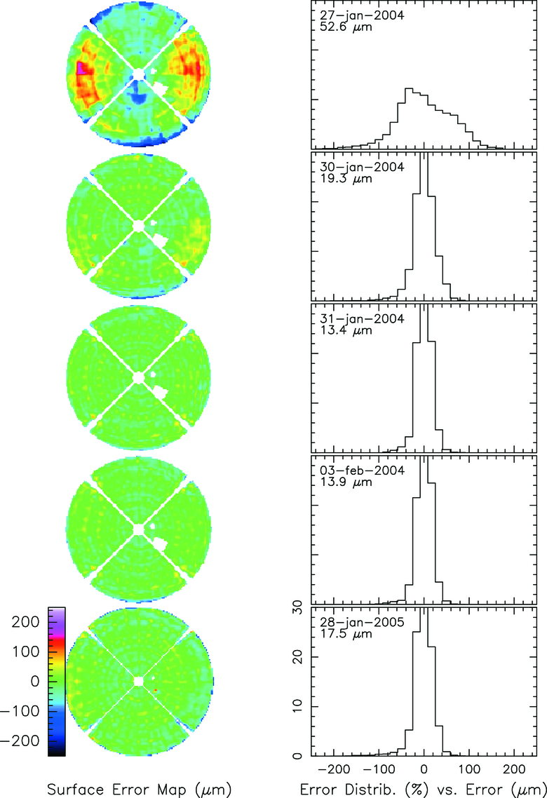
Fig. 6.— Sequence of surface error maps with intermediate panel setting for the AEC antenna. The surface contours are shown on the left side, the error distribution on the right. The white cross and the small white area represent the quadripod and a faulty panel and were not considered in the calculation of the rms error.
The adjustments were done with a tool provided by the contractor. It was similar to the one used by us on the VertexRSI antenna, but it was calibrated in "turns" rather than in microns. Again, two people on a man‐lift approached the surface from the front, where the adjustment screws are located. The time needed for an adjustment of the total of 600 adjusters was 7 hr, well within the specification of 8 hr.
5.1.2. Temporal Surface Stability
VertexRSI antenna: To estimate the accuracy and repeatability of the measurements, we produced difference maps between successive measurements throughout the measurement period. The rms difference between consecutive maps is typically less than 10 μm, and usually ∼8 μm. An example of a difference map is shown in Figure 7. The map of measurement number 307 is shown on the left, while the right panel shows the difference between map 307 and 308, made about 1 hr later.
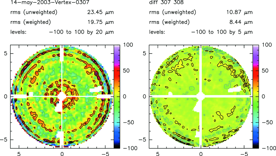
Fig. 7.— Example of the repeatability of the VertexRSI holography measurements. The map on the right is the difference between the one at left and a map made 1 hr afterward. The rms of the difference maps is about 8 μm, which is commensurate with the expected value due to noise and atmospheric fluctuations.
We have made many maps after the final setting of the surface, changing the orientation of the antenna with respect to the Sun. Maps taken over a few consecutive days were obtained at widely different temperatures and while the wind conditions varied over time. The measured rms error during a 30 hr period in early 2003 May varied between 20 and 23 μm. During this period, the wind was calm (<5 m s−1) and temperature changes of 15°C were encountered. A later 5 day series in mid‐June gave rms errors from 22 to 26 μm, with temperature variation up to 20°C, wind speeds up to 10 m s−1, and periods of full sunshine. Most of this increase is believed to be due to the deteriorating atmospheric conditions at the VLA site during summer, when the humidity was significantly higher than normal. The much better results of 17 μm obtained during the cold and dry winter period also point to a significant atmospheric component in the spring and summer results.
However, some of the changes will be caused by temperature and wind. To increase the rms from 20 to 22 μm, the "additional" component needs a magnitude of 9 μm rms. Such a contribution can be expected from the calculated values of 4 μm each for wind and temperature for the panels, and 5 μm for wind and 7 μm for temperature for the BUS. These numbers are all within the specification. Actually, the measured differences are close to those expected from the estimated accuracy of the holography measurement and the measured rms differences in consecutive maps of about 8 μm.
AEC antenna: In Figure 8 we show one of the final results and a difference map of this and the following measurement, made 1 hr later. The difference map indicates a repeatability of ∼5 μm rms. There is no indication of the wavy structure in the outer region of the aperture, as was the case for the VertexRSI antenna. We ascribe this to the lower signal level due to the long piece of waveguide between feed and mixer.
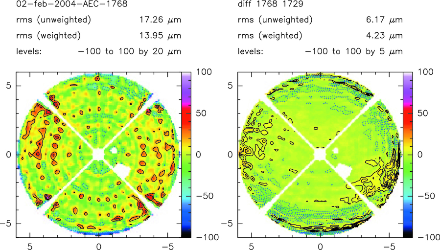
Fig. 8.— Same as Fig. 7, but for the AEC antenna, and with an rms of 5 μm for the difference maps.
We made a series of 16 maps over a period of more than 2 days in early 2004 February. Temperatures ranged from +2°C to −10°C, while the wind was mostly calm, with some periods of speeds up to 10 m s−1. During one day, there was full sunshine. The measured rms error is very constant, with a peak‐to‐peak variation of less than 2 μm on an average of 14 μm. The differences are fully consistent with the allowed errors under environmental changes, and they are also of the same order as the measurement accuracy. We believe that the significantly better overall result is mainly due to the much drier and more stable atmosphere during these measurements as compared with the summer data from the VertexRSI antenna.
5.1.3. Surface Stability with Changes in Ambient Temperature
VertexRSI antenna: Further analysis of the VertexRSI time‐series data presented in § 5.1.2 has been made in order to extract the dependence of the antenna surface on changes in ambient temperature. The analysis entailed the following:
- 1.For each series, the average of all maps in the series was subtracted from all the maps in the series. This suppresses dependencies on any long‐term effect.
- 2.In each series, the maps were divided into several temperature ranges; in each temperature range, the average map was computed.
- 3.Finally, the differences between the coldest and warmest range averages were computed for each series. From these data, we derived the surface deformation caused by a temperature change of 10°C, as shown in Figure 9.
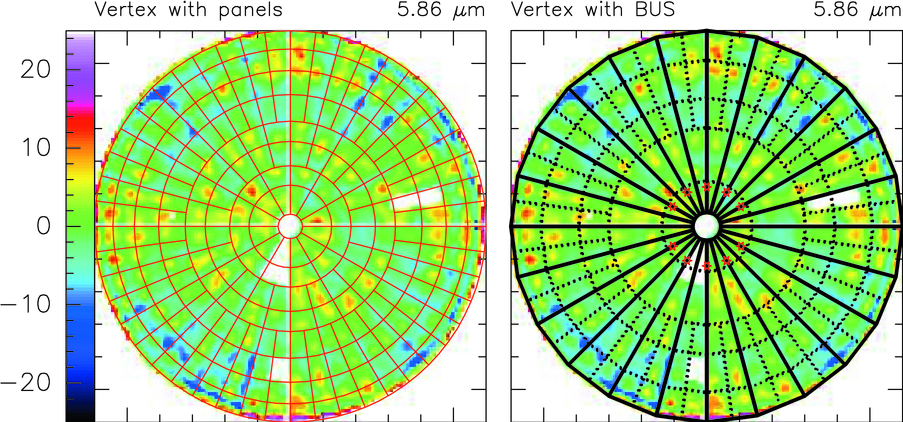
Fig. 9.— VertexRSI temperature span plots with panels (left) and BUS (right) boundaries overlaid. To put these measurements on the same scale, the data have been uniformly scaled to a temperature difference of 10°C. The rms surface deformation over this 10°C temperature difference is indicated at top right.
From this analysis, we note that
- 1.Many of the samples were for temperatures outside the primary operating range of −20°C to +20°C.
- 2.The results for the spring 2003 and winter 2005 periods are very consistent with each other.
- 3.The magnitude of the rms deformations is ∼0.6–0.7 μm K−1. This value seems high. It is not clear to which degree it should be split into panels and BUS and between absolute and gradient terms in the surface error budget. Assuming all effects to be linear with temperature, and antennas set at 0°C, we would expect rms temperature contributions of ∼13 μm for the VertexRSI antenna at either end of the operational temperature range (+20°C or −20°C).
- 4.The thermal deformations for the VertexRSI antenna appear to be a mixture of BUS (the BUS sector edge sticks out at higher temperature) and panels, not all panels deforming equally.
- 5.From the BUS overlay drawing (Fig. 9), it appears that there is a print‐through of the connections of the BUS with the Invar cone (the turnbuckles). The small red islands on (or just outside) the second stippled ring are at the diameter of the outer support of the BUS on the cone. We are not certain whether they are at or between the connections to the cone. In both cases, such a print‐through might reasonably be expected.
- 6.The BUS is also supported on the cone toward the center, outside the inner stippled circle by about one‐fifth of the distance between the two stippled circles. Here we also see clear red islands of print‐through. These effects are less pronounced in the lower section of the dish; actually, they seem most pronounced in the left and right quadrants. We do not understand why this would be the case.
- 7.There are clear, narrow "valleys" along the radials where the sectors of the BUS are joined, especially in the outer half of the radius. They are not equally strong all around, but are visible in most cases. The inner part is less clear, presumably because of the already existing effects of the support points.
- 8.From the map with the panel outline, and ignoring the islands connected to the BUS, as argued above, there is some but not very much evidence for individual panel deformations. It is most likely the case that individual panel deviations are caused more by forces originating in the stiffer BUS than from the panel itself.
AEC antenna: Further analysis of the AEC time‐series data presented in § 5.1.2 has been made in order to extract the dependence of the antenna surface on changes in ambient temperature. The analysis entailed the same sequence of calculations as those presented for the VertexRSI antenna (see § 5.1.3). Figure 10 shows the temperature span assuming a uniform 10°C temperature difference.
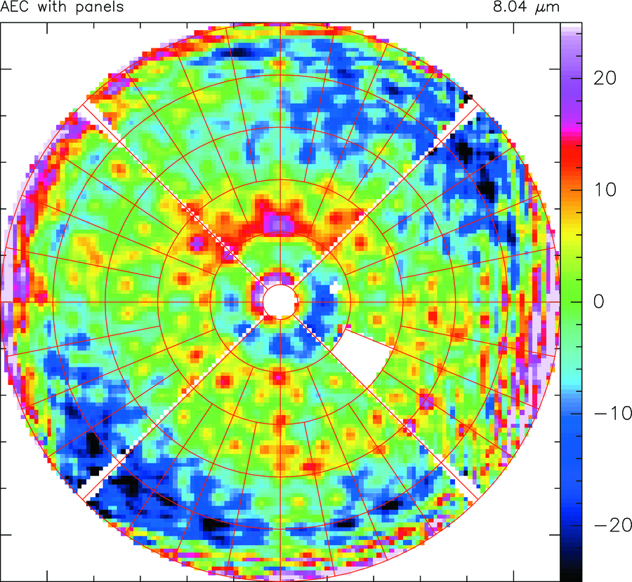
Fig. 10.— AEC temperature span plot with panel boundaries overlaid. Measurements are scaled as in Fig. 9.
From this analysis, we note that
- 1.The sampled temperature range is completely inside the primary operating condition ambient temperature range of −20°C to +20°C.
- 2.The magnitude of the rms deformations is ∼0.8 μm K−1. This value seems high. It is not clear to which degree it should be split into panels and BUS and between absolute and gradient terms in the surface error budget. Assuming all effects to be linear with temperature, and antennas set at 0°C, we would expect rms temperature contributions of ∼16 μm for the AEC antenna at either end of the operational temperature range (+20°C or −20°C).
- 3.The large‐scale deformation at a 45° position angle (which looks like astigmatism), along with the additional deformation of the inner ring, are hard to explain. These deformations are perhaps due to the temperature gradients in the cabin and the BUS, coupled to the quadripod connection points. The vertical stripes on the edges of the AEC maps are an artifact of the measurement that is not related to temperature.
- 4.In principle, there should be little print‐through structure in the difference maps, due to the fact that the BUS design is more homogeneous, being all CFRP, and it should have a continuous transfer of forces to the cabin, which is also of the same material.
- 5.We do not see any individual panel deformation.
5.2. Near‐Field Holography Measurement Conclusions
- 1.The holography system has functioned according to specification and has enabled us to measure the surface of the antenna reflector with a repeatability of better than 10 μm.
- 2.
- 3.The small differences in the surface maps obtained over several days of measurement are consistent with the measurement repeatability and at best are marginally significant. If taken at face value, they indicate that under varying wind and temperature influences, the deformations of the reflector are fully consistent with and probably well within the specification. This excellent behavior over time is more important than the actual achieved surface setting. We stopped iteration of the settings after having achieved the goal of less than 20 μm.
- 4.The measured variations with ambient temperature changes appear somewhat large. They correspond to a thermal contribution to the surface error of 10–16 μm at the boundaries of the operational range (−20°C and +20°C), assuming a setting at 0°C. This is slightly more than the contribution in the "ALMA error budget" and also more than the prototype antenna contractors have budgeted. On the other hand, taking BUS, panel, and adjuster error contributions altogether leads to approximate agreement with these measurements.
- 5.Within the primary operating range of −20°C to +20°C for ambient temperature, the surface error budget of the production antennas allows for a BUS contribution of 8 μm due to absolute temperature change, and 7 μm for gradients. The panels are allowed 4 μm for absolute temperature and temperature gradient each. If we assume that the surface is set at 0°C to a measured value of 15 μm, which is the value we achieved, and we add the 15 μm maximum of the temperature deformation, the resulting error is 22 μm. This is higher than the goal, but well within the specification. High mountain sites, including Chajnantor, generally experience wind. This will dampen temperature gradients in the antenna structure and hence decrease the resulting structural deformation.
5.3. Accelerometer Measurements of BUS Deflection
Accelerometers are used to measure accelerations in the inertial coordinate system of the antenna, allowing for the determination of rigid body motion of the elevation structure, as well as a few low‐order distortions of the BUS. In addition, motion of the subreflector structure with respect to the BUS can be measured. For the BUS deformation measurements, 10 accelerometers were placed on the BUS in the following configuration (Fig. 11):
- 1.Three accelerometers as a three‐axis sensor on the subreflector structure (labeled A1–3 in Fig. 11).
- 2.Four accelerometers along the rim of the BUS in the boresight direction (A4–7).
- 3.Three accelerometers as a three‐axis sensor on the receiver flange Invar ring (A8–10).
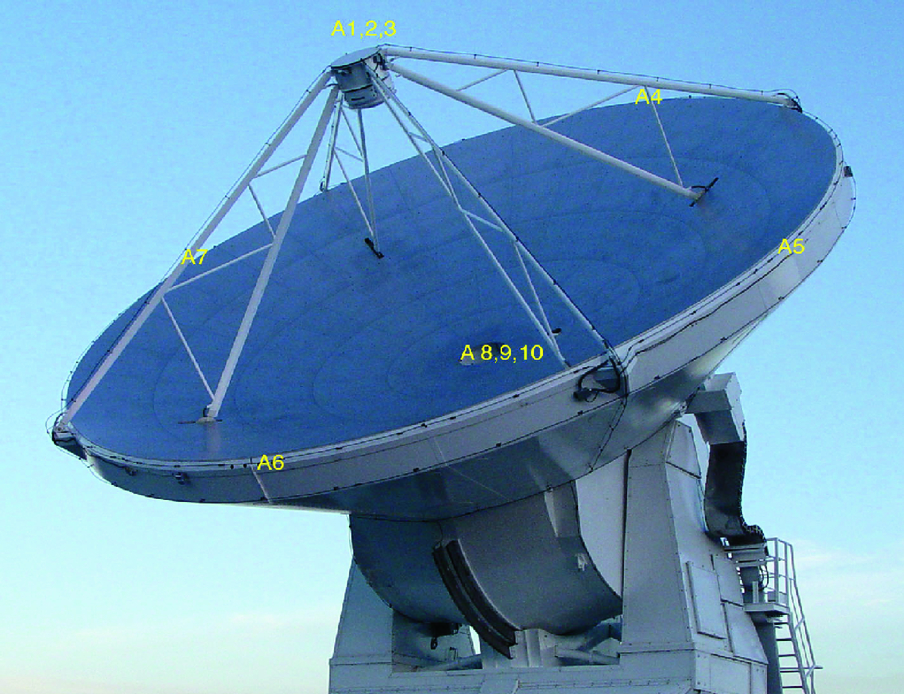
Fig. 11.— Placement of the accelerometers on the antenna for BUS deflection (surface accuracy) measurement.
The nature of the accelerometers used here limits accurate displacement measurement to timescales of at most 10 s or frequencies of at least 0.1 Hz. Since this is well below the lowest eigenfrequencies of the antennas, this is sufficient to determine dynamic antenna behavior. See Snel et al. (2006) for further information about the ALMA accelerometer measurement system.
Over the 0.1–30 Hz sensitivity range of the accelerometers, the changes in reflector surface shape through measurements of the focal length (Zernike polynomial Z3 "power," "defocus" term, n = 2, m = 0) and "+" astigmatism (Zernike polynomial with n = 2, m = 2) can be measured to better than a few microns.
5.4. BUS Deflection Measurement Conclusions
For 9 m s−1 wind over timescales of 15 minutes, the VertexRSI antenna surface is stable to 5.3 μm astigmatism rms at the rim of the BUS, and 2.2 μm defocus. The AEC antenna surface is stable to 6 μm astigmatism rms at the rim of the BUS, and 5 μm defocus. For both antennas, surface stability is dominated by the stiffness of the BUS for wind excitation at low frequencies. The measured values are in reasonable agreement with the error budget numbers from the contractors. Note that these values do not include gravitational and thermal effects. During sidereal tracking, the astigmatism and defocus deformations remain below 1 μm for both antennas.
A frequently used operational mode of ALMA is "fast switching," in which the antennas are pointed alternately at the observed source and a nearby calibration source 1°–2° away, typically at 10 s time intervals. The antennas are designed to achieve such a switch within 1.5 s. It is of interest to measure the dynamical behavior of the antenna structure during such switching cycles. During the strongly accelerated and decelerated movement, we measure negligible BUS rim deformations of the order of 1 mm, which decrease to a few microns after the new position has been reached.
During on‐the‐fly (OTF) observing, the antenna scans a region of sky back and forth at a speed of 0 5 s−1. During this movement, we measure astigmatism at the reflector edge and a defocus movement of a few microns each. Interferometric mosaicking at 005 s−1 causes barely measurable astigmatism and a defocus stability of about 1 μm.
Within the sensitivity of these measurements, it can be stated that both antennas exhibit dynamical deformations of the reflector surface that are small and in agreement with the surface error budget. In addition, as these measurements demonstrate, very small dynamical deformations can reliably be measured with this accelerometer setup. We consider this method, pioneered by Ukita & Ikeda (2002) and also used on an optical telescope by Smith et al. (2004), of great potential for the study of the dynamical behavior of large and highly accurate telescopes.
6. ABSOLUTE AND OFFSET POINTING
In the following section, we describe the analysis of the pointing performance of the two ALMA prototype antennas. The analysis is (mostly) based on optical pointing observations carried out between 2003 October and 2004 May and radio pointing measurements carried out during 2004 March (VertexRSI) and May (AEC). The optical and radio pointing data analysis was carried out using the proprietary TPOINT telescope pointing analysis software. The AEC results are more limited than those from the VertexRSI antenna and cover a shorter time span, because of the late handover of that antenna.
This pointing analysis studies three aspects of the antennas:
- 1.All‐sky blind pointing accuracy.
- a)In the optical case:
- i)Find the model that best describes the all‐sky pointing for the antenna under study, in its "optical pointing test configuration."
- ii)Find the best coefficient values for use in the seven‐term ALMA "standard internal model" (§ 6.1.2).
- iii)Estimate the best all‐sky optical pointing performance that could be expected operationally (§ 6.3).
- iv)Assess the stability of the optical pointing model (§ 6.3.4).
- b)In the radio case:
- i)Find the model that best describes the all‐sky pointing for the antenna in question when operating in its radio configuration (in particular at 95 GHz).
- ii)Estimate the best all‐sky pointing performance that could be expected operationally.
- 2.Assess the smoothness of tracking (optical and for one antenna only).
- 3.Determine the ability to offset accurately across short distances (optical only).
In all, the pointing analysis of the ALMA prototype antennas relied on measurements made with three distinct systems:
- 1.An optical pointing telescope (OPT) mounted within the BUS of each antenna. The OPT is a NRAO‐designed refracting telescope composed of a 4 inch (10.16 cm) lens mounted within a rolled‐Invar tube (J. Mangum 2004; see footnote 6). The detector used was a commercial CCD camera coupled to a video frame grabber. Figure 12 shows two typical absolute (all sky) pointing residual plots obtained with the OPT system.
- 2.Radiometric measurements at 1 and 3 mm wavelength. Figure 13 shows a sample single‐dish image obtained with this receiver system.
- 3.An accelerometer system (§ 6.8).
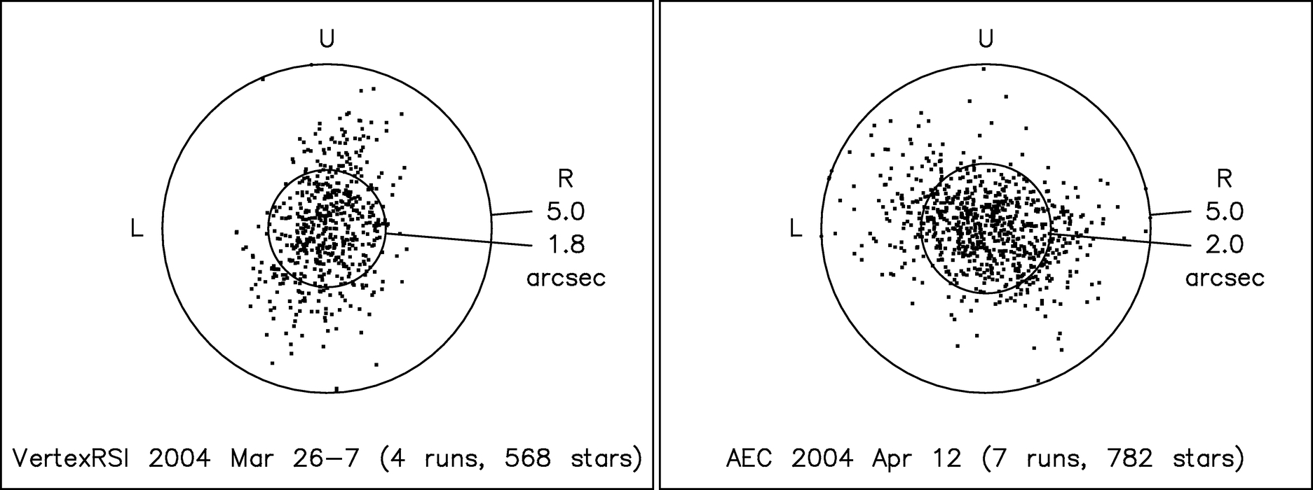
Fig. 12.— Sample VertexRSI (left) and AEC (right) OPT pointing residual plots showing the measurement residuals following application of the respective pointing models, each composed of 13 terms. The outer ring marks a radial residual of 5'', while the inner ring indicates the rms pointing residual for each antenna.
Both prototype antennas were designed to meet the pointing specifications with the aid of various metrological correction systems. These metrology systems were generally unsuccessful at improving the pointing performance of the prototype antennas, as described in § 6.6.
6.1. Pointing Models
6.1.1. TPOINT Modeling
If a telescope or antenna is pointed at a star, there is generally a difference between the true direction of the incoming light and the demands to the mount servos, due to mechanical misalignments, flexures, and other imperfections. By observing stars all over the sky and logging the actual and commanded positions (or data from which these angles can be deduced), a mathematical model can be developed that estimates the servo inputs required to point the antenna accurately in a given direction. The TPOINT pointing analysis software reads a file containing the logged observations and provides graphics and modeling tools that allow a mathematical description of the pointing errors to be created. The resulting pointing model then has to be built into the telescope or antenna control system so that the demands to the servos are appropriately adjusted and the accurate dead‐reckoning acquisition of celestial targets is brought about.
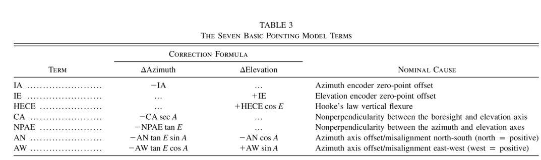
For any two‐axis gimbal mount, the basic a priori model consists of seven terms: two encoder index errors, two nonperpendicularities, two azimuth‐axis tilt components, and Hooke's law flexure. All of these terms have a clear mechanical interpretation, and in general, all will be present to some degree. This basic model usually performs well, typically leaving only a small remaining systematic residue to be mopped up using the repertoire of other TPOINT terms. Most of the latter set out to represent plausible mechanical effects—for example, harmonic terms to deal with runouts and mechanical deformation errors—although it is also possible to introduce unashamedly empirical terms such as polynomials, should there be no alternative.
The functional form of the basic seven‐term model is given in Table 3. The following should be noted:
- 1.The sign of the correction terms is such that the expressions should be subtracted from the true direction in order to generate mount demands.
- 2.The coefficient values in service will either be those from the most recent set of observations or averages of several recent runs.
- 3.The expressions are approximate, which is adequate when the coefficients are small or the target is not too close to the zenith. TPOINT in fact fits rigorous vector formulations that do not have these limitations.
 |
6.1.2. The Standard ALMA Internal Model
The a priori seven‐term model (Table 3) is also that specified by ALMA for internal implementation in the low‐level antenna controllers, principally as an aid to commissioning. Once the final TPOINT model is available, the optimum coefficients to be used with this basic seven‐term model can be estimated by subtracting the full model from a set of points distributed evenly over the sky, and then fitting the seven‐term model. The final rms from such an experiment represents the maximum achievable performance of the ALMA internal model for the antenna in question, while the residual plots illustrate the antenna's pointing idiosyncrasies. This experiment was carried out for both antennas, using OPT data, for illustrative purposes. For the AEC antenna, the best‐fit sky rms was 246, while that for the VertexRSI antenna was 325. The limitations of this simple seven‐parameter model are illustrated in Figure 14.
6.2. The ALMA Optical Pointing Telescopes
Optical pointing systems have become standard equipment on millimeter and submillimeter telescopes. There are benefits and limitations associated with the reliance on optical pointing systems on radio telescopes:
- 1.Benefits
- a)There are many more bright stars that can be used as optical pointing sources than radio pointing sources.
- b)With a CCD camera, optical data acquisition can be done on timescales as short as a few tenths of a second, as opposed to the tens of seconds timescales necessary for radio pointing measurements.
- c)Positions of optical stars can be derived to subarcsecond accuracy, which is a much higher precision than that obtainable through single antenna radio measurements.
- 2.Limitations
- a)Differences between the position and behavior of the optical and radio signal paths can make it difficult to derive the radio pointing coefficients from optical pointing measurements.
- b)Optical pointing is not possible during overcast weather conditions.
- c)Optical pointing cannot be used in the daytime, unless the system has been designed with near‐infrared sensitivity.
Optical pointing systems find application in such areas as (1) pointing and tracking diagnosis, (2) pointing coefficient derivation and monitoring, and (3) autoguiding.
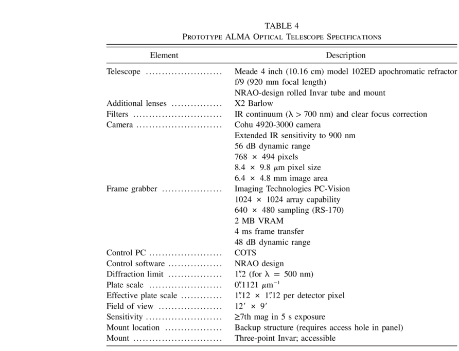
Table 4 lists the ALMA prototype optical telescope system specifications (J. Mangum 2004; see footnote 6).
 |
6.2.1. Optical Telescope Measurement System Limitations
- 1.The optical seeing at the VLA site is generally poor. To quantify this seeing contribution to the OPT measurements, a sequential multiple star measurement, in which each star measurement was repeated three times, was used to derive seeing and short‐timescale antenna positioning errors. These measurements suggest a seeing/vibration contribution of ∼15, in line with the results from tracking tests. With the OPT's 100 mm aperture, the seeing manifests itself as large and rapid movements of the image, making optical measurement of the all‐important tracking and offsetting performance almost impossible.
- 2.The OPT design, which was always going to be a major challenge, is itself marginal for this application, given the impressive performance of the antennas. The comparatively short focal length means that the image is undersampled, and in some of the tracking tests, quantization effects are evident, making performance limitations much below 1'' difficult to detect. It is far from obvious how to deal with this; a refracting OPT of, say, twice the aperture would have been prohibitively expensive and also very large, whereas a reflector (a commercial Schmidt‐Cassegrain, for example) would probably have had insufficient optical stability.
6.3. Optical Pointing Telescope Measurements
6.3.1. Data Acquisition
The pointing measurement data logging procedure evolved during the antenna evaluation process, ultimately leading to a very self‐consistent and robust scheme for position calculation and logging. We refer to this final position calculation and logging scheme as PMDR (pointing model done right).
The two schemes (pre‐PMDR and PMDR) are illustrated in Figure 15. In the pre‐PMDR mode, the inputs to the TPOINT pointing analysis are (1) the "observed" azimuth and elevation (i.e., the true line of sight) and (2) the encoder readings from the mount axes. The TPOINT analysis produces updated pointing coefficients for the ALMA internal seven‐term model, calculated to minimize the offsets required to peak up on a new source and, equivalently, the drifts during subsequent tracking. However, note that coefficients obtained in this way presume zero metrology input; they are not suitable for use with metrology enabled, and the fitting statistics (e.g., rms) do not reflect any benefits coming from the metrology system. Moreover, if the control system supplied by the manufacturer were to be used, the TPOINT model would be limited to the seven standard terms (from Table 3), and additional forms of correction would not be available. This final point proved to be a major handicap, hampering the pointing performance characterization of the ALMA prototype antennas and limiting the ultimate performance (see Fig. 14).
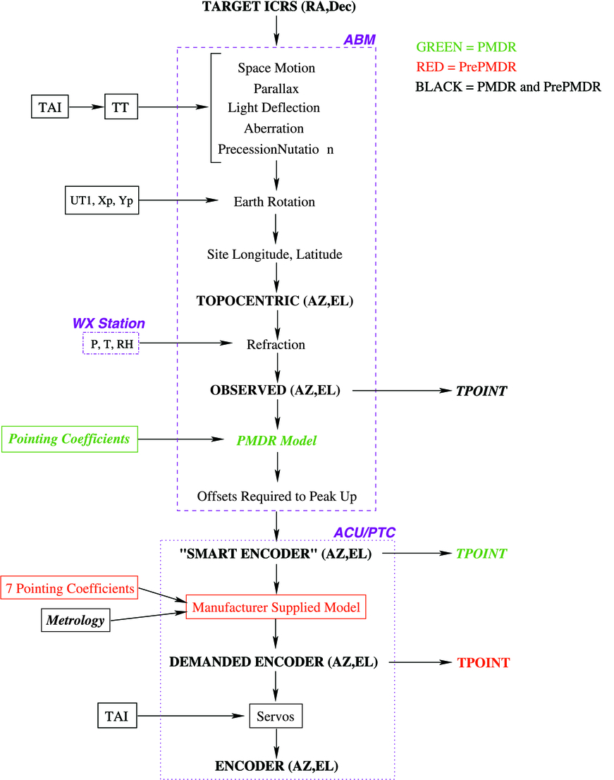
Fig. 15.— Positioning calculation flow chart for the pre‐PMDR and PMDR systems. The roles of the respective computers are shown in boxes.
These shortcomings were addressed by the PMDR scheme (Fig. 15, green items). In this scheme, the quantities logged for input to TPOINT are (1) the observed azimuth‐elevation (or az‐el) as before, but this time including (2) the commanded inputs to the manufacturer's model and metrology systems, the latter constituting a "smart encoders" interface. The link between the two is a separate TPOINT model that can contain any required terms, not just the seven basic terms. In fact, it is advantageous to disengage the manufacturer's model so that the TPOINT model provides the whole correction, apart from the metrology inputs: the end result is the same, and the TPOINT model then represents absolute physical estimates (nonperpendicularities, misalignments, flexures, etc.). All measurements quoted in the following analysis used the PMDR positioning and logging scheme.
6.3.2. All‐Sky Optical Pointing Data
The respective data samples for each prototype antenna are listed below. For both samples, we note that
- 1.The short time span available for evaluating pointing performance unfortunately precluded any studies of the long‐term stability of the pointing terms.
- 2.A handful of these pointing tests were carried out with contractor‐delivered metrology systems. We describe the results of these few metrology tests in § 6.6.
- 3.To obtain the total sample of measurements for both antennas, individual runs were for the most part accepted or rejected on the basis of notes made at the time they were carried out, rather than whether they gave better or worse pointing residuals. However, certain runs were clearly aberrant. These obviously atypical runs were rejected.
AEC: A selection of 63 pointing test runs were carried out during an intensive period of testing between 2004 March 6, when the antenna first became available, and May 12. There were a total of 7411 observations in this sample. Following some modifications by the antenna contractor in 2004 December, an additional series of measurements were made during the period of 2005 January 7 to March 2. As these additional measurements are not directly comparable to those made during the 2004 March 6 through May 12 period considered here, we defer their analysis to § 6.3.5.
VertexRSI: A selection of 34 pointing test runs that utilized the PMDR positioning system (see § 6.3.1) were carried out between 2004 March 10 and May 3, comprising 4059 observations.
6.3.3. The OPT Core Terms
In the final optical‐pointing–derived models, we have distinguished a set of floating basic pointing terms (IA, IE, CA, AN, and AW) from a fixed "core" set of terms that are not only considered to have a specific mechanical cause, but can also be assumed to be fixed in size. Moreover, for most of these core terms, there is no reason to suppose that they will be affected by the transition from optical to radio pointing.
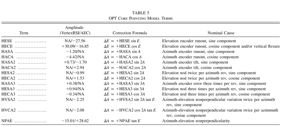
The core terms for both prototype antennas are listed in Table 5. For each term, we list the nominal mechanical deformation that produces the term. Note the following:
- 1.The sign of the correction terms is such that the expressions should be subtracted from the true direction in order to generate mount demands.
- 2.The smallest terms are of order of 1'' and 05 in size for the AEC and VertexRSI models, respectively. Their significance can be gauged by eliminating the smallest of them, namely HESA2 (AEC) and HECA3 (VertexRSI), fitting the full model to take up the slack, and plotting the residuals. The result of this experiment shows a distinct sin (2A) (AEC) and cos (3A) (VertexRSI) systematic residual in Δelevation versus azimuth for the respective antennas. Figure 16 shows the graphical results for the AEC antenna.
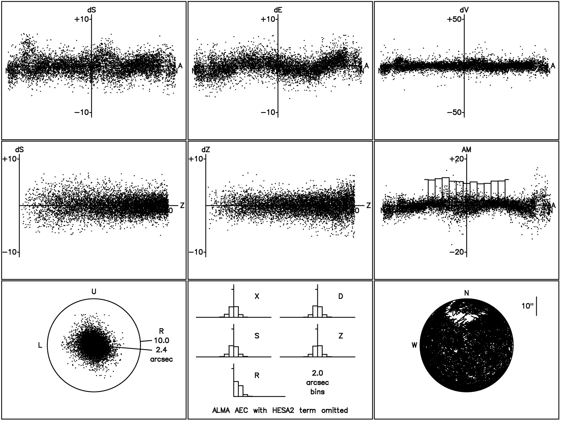
Fig. 16.— TPOINT plot showing the significance of the HESA2 term for the AEC antenna pointing model. Note the clearly systematic residual in Δelevation vs. azimuth in the top center panel, suggesting the need for a sin (2A)‐dependent term.
 |
6.3.4. Stability of the OPT Pointing Model
In principle, all of the terms of an antenna's pointing model should maintain constant amplitude for long periods unless something on the antenna has been adjusted. This supposition was studied by taking the individual models for the series of pointing tests on each antenna and plotting the coefficient values for the five terms thought most likely to be affected by mechanical adjustments and drifts. The stability of these coefficient values was then studied by plotting them versus sequence number (in effect vs. time).
For the AEC antenna, the stability of the five basic pointing model terms over the period of 2004 March 6 through May 12 was (ΔIA, ΔIE, ΔCA, ΔAN, ΔAW) = (±3'', ±5'', ±3'', ±1'', ±1''), with very little drift of the average values for each term. This is very good basic pointing term stability for an antenna. The VertexRSI antenna pointing term stability over a much longer measurement period (2003 October 16 to 2004 March 1) was (ΔIA, ΔIE, ΔCA, ΔAN, ΔAW) = (±3'', ±7'', ±5'', ±5'', ±3''), with very little drift of the average values for most terms (the AN term showed a moderate ∼5'' drift of the average during the measurement period). The basic pointing‐model‐term stability for the VertexRSI antenna was notably worse than that of the AEC antenna. Part of this poorer performance is likely attributed to the failure of the tiltmeter metrology system (see § 6.6), which was designed to correct for variations in the azimuth axis tilt (AN and AW).
6.3.5. Additional OPT Measurements of the AEC Antenna
Following the all‐sky OPT measurements described above, the antenna contractor made some modifications designed to improve the all‐sky pointing performance. In particular, the attachment points of the antenna base to its foundation were tightened, and a tiltmeter‐based metrology correction was enabled in an attempt to correct the suspected instability in the azimuth bearing. An additional series of measurements were made during the period of 2005 January 7 to March 2 following these modifications. From these measurements, we note that
- 1.Two terms (HVSA2 and HVCA2) were no longer significant and need not exist in the pointing model solution. The terms HVSA2 and HVCA2 represent changes in the az‐el nonperpendicularity as the mount rotates. The insignificance of these terms suggests that the azimuth axis had become less wobbly.
- 2.Figure 17 shows the cumulative AEC optical pointing model results for this period. For each total rms value shown, we also show the contributions to this total rms due to cross‐elevation and elevation pointing residual.
- 3.A large observed shift in the IA and AW pointing terms relative to the previously derived pointing models reported in P. Wallace et al. (2004; see footnote 4) was ultimately diagnosed as a timing error of approximately 13 s in the monitor and control system. This timing error does not affect the resulting pointing rms values derived. On 2005 January 20, this timing error was corrected.
- 4.A timing signal cable problem was fixed on 2005 January 23.
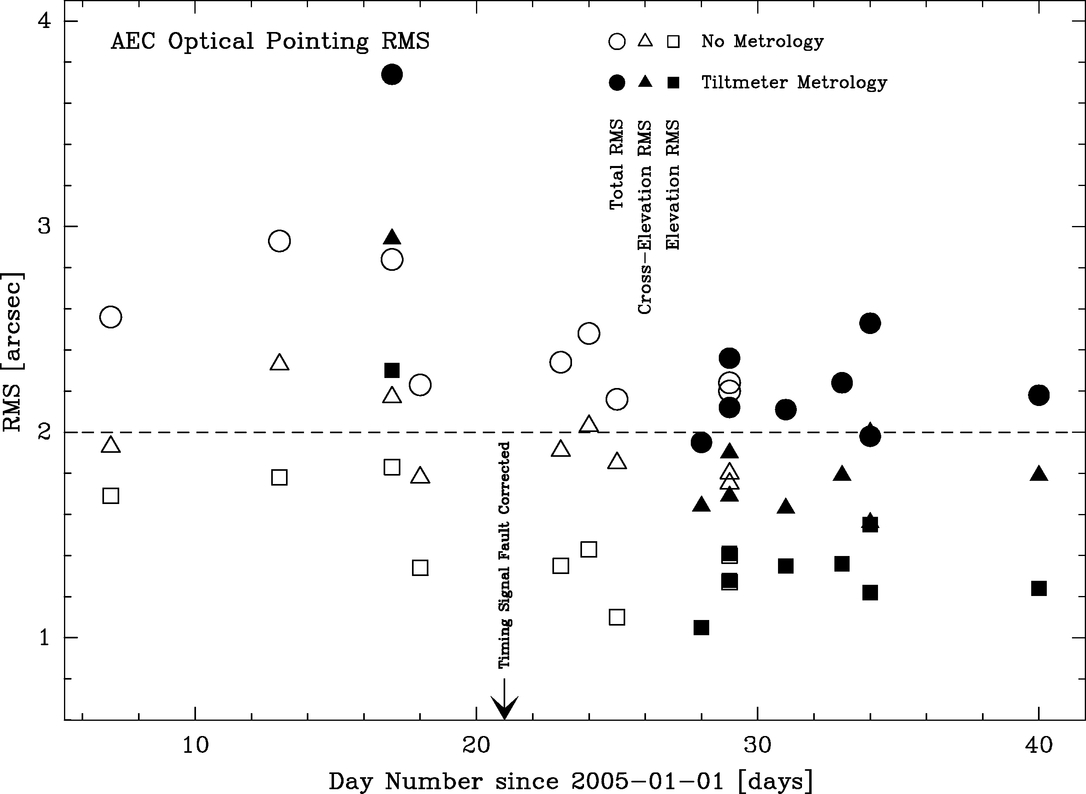
Fig. 17.— AEC optical pointing results for the period 2005 January 7 to 2005 March 2.
6.3.6. Pointing Model Recalibration Frequency
The ALMA pointing specification permits monthly recalibration of the pointing model. To investigate this, two representative all‐sky OPT runs taken a month apart were chosen. The first was used to simulate the periodic recalibration of the five "noncore" terms of the AEC model (IA, IE, CA, AN, and AW). This simulated operational model was then applied to the second data set, and the resulting pointing performance was assessed with various terms refitted, as might be done in a quick daily recalibration.
Operationally, the frequent observation of standard stars means there is an opportunity to adjust at least the boresight offsets more frequently, and this was simulated by allowing the terms IE and CA to float. For AEC (VertexRSI), they changed by 29 (146) and 17 (15), respectively, and gave sky rms values of 244 (305), still somewhat outside the specification.
If the tilt terms AN and AW were also allowed to vary, the changes for AEC (VertexRSI) were 13 (18) and 00 (24), respectively, and the sky rms values were 222 (185), somewhat better and well within the specification for the VertexRSI antenna. This is an indication of the improvement that correctly working metrology (base tiltmeters) would offer.
With the azimuth zero‐point term IA added, completing the standard five floating terms, the sky rms reduced only slightly, to 216 for the AEC antenna, and was unchanged for the VertexRSI antenna. However, a significant improvement in the fit to the AEC measurements, to 195 rms, occurred when the az‐el nonperpendicularity term NPAE was included in the fit. The changes in the IA and NPAE terms for the AEC antenna were 112 and 126, respectively, and may be evidence of the suspected azimuth bearing instability in this antenna.
The conclusions were as follows:
- 1.Some form of rapid recalibration (say, daily) will be needed in addition to any relatively infrequent full calibration.
- 2.Frequent recalibration of the boresight offsets IE and CA is essential.
- 3.Recalibration of the tilt terms AN and AW is also essential for the VertexRSI antenna performance, unless correctly functioning base tiltmeters can render this superfluous.
- 4.Even with frequent recalibration of the boresight offsets, the AEC antenna performance would not quite reach the 2'' specification.
6.3.7. Optical Tracking Tests on the VertexRSI Antenna
A pointing run consisting of observations of a single star for about 45 minutes was used to test antenna tracking performance. Because only a small region of sky was observed (a line about 10° long), the data set is not suitable for fitting a pointing model. Although it turns out that doing so produces a sensible model, there is a danger of fitting out some of the tracking error that the experiment is designed to expose. Accordingly, an all‐sky pointing run acquired during the following day was used instead. Applying this model to the tracking test and allowing only a zero‐point correction (i.e., the TPOINT terms IE and CA) produced a sky rms of 146 and the ΔAcos E and ΔE tracking residuals shown in Figure 18 (the x‐axis is sequence number and hence time).
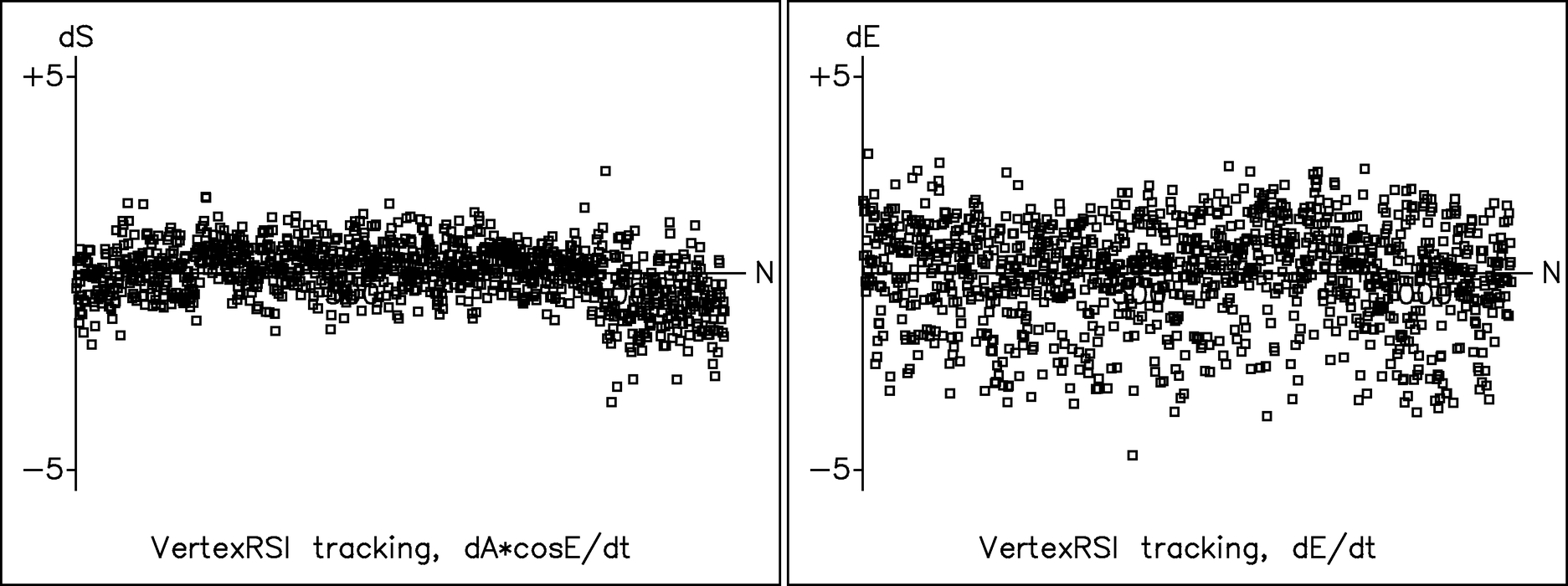
Fig. 18.— Tracking errors for the VertexRSI antenna. The x‐axis is sequence number and hence time.
Note the following:
- 1.The scatter up‐down is larger than left‐right and is not normally distributed; the larger deviations tend to be downward on the plot.
- 2.Beneath the noise, both axes show slow drifts. However, these are very small, barely 1'' peak to peak. They might be the underlying errors in the pointing model, in its variance from day to day and (if temperature plays a role) from hour to hour, or they could be anomalous refraction or changing wind pressure. They happen too slowly to affect the ability to offset accuracy over short timescales, but do perhaps suggest that small adjustments to the pointing model on timescales of a few tens of minutes may be a wise precaution.
- 3.The noise is of such high frequency that it is not what would usually be thought of as tracking error. This high‐frequency noise is more of a "jitter" and is likely caused by the seeing‐induced movements of the optical image, rather than the smoothness of the antenna motion.
- 4.There is a fairly abrupt change in the left‐right tracking near the end of the run, and hints of other relatively high frequency artifacts. If such events can happen during offsetting maneuvers, the 06 in 2° science requirement might be in jeopardy. However, if the typical tracking were an illustration of the offsetting performance, then the 06 figure would be easily achievable. In other words, in a typical 2° portion of the tracking plot, the drift is within that figure. The largest slope on the elevation plot, for example, corresponds to about 2'' in the total of 11° of track, or about 04 per 2°. The slopes on the ΔAcos E track are somewhat steeper if we overlook the high‐frequency events.
6.3.8. All‐Sky Optical Pointing Summary
- 1.The rapid slewing of the ALMA antennas leads to data sets of ample size compared with the five or six variable terms of the model, and so the rms figure is a good guide to the population standard deviation.
- 2.All‐sky optical pointing measurements made over ambient temperatures from −10°C to +20°C and for wind speeds ranging up to 17 m s−1 show no dependence on either of these site conditions.
- 3.For the AEC antenna, the all‐sky rms pointing accuracy from the 2004 March 6 through May 12 period (Fig. 19) is typically 24, with the better results in the first half of the test period, which was when the more stable IE and CA values were seen.
- 4.In Figure 19, the AEC sky rms is resolved into two components, left‐right and up‐down. It is evident that the left‐right component (i.e., ΔAcos E) is worse than the up‐down component (i.e., ΔE). This worse azimuth behavior is fairly constant over the test period, whereas the unexplained decline in elevation performance in the second half accounts for most of the deterioration in overall rms.
- 5.Figure 17 shows the AEC all‐sky rms pointing accuracy for the period of 2005 January 7 and March 2. The mechanical modifications made by the antenna contractor have produced a moderate improvement to the all‐sky pointing performance.
- 6.For the VertexRSI antenna, Figure 20 shows that if we neglect the earlier, pre‐PMDR period, the sky rms is not much affected by the passage of time and changing conditions. A typical result is 20 rms, and most of the PMDR runs delivered better than this, in some cases much better. Figure 20 also shows the sky rms resolved into two components, left‐right and up‐down. It is evident that the up‐down component (i.e., ΔE) is worse than the left‐right component (i.e., ΔAcos E). The performance variations in the two axes seem to be somewhat correlated, perhaps evidence that variations in optical seeing were involved, while the occasional poor sky rms happened when there was a sudden worsening in elevation performance.
- 7.A sequential multiple star measurement, where each star measurement was repeated three times, was used to derive seeing and/or short‐timescale antenna positioning errors. These measurements suggest a seeing/vibration contribution of ∼15, in line with the results from radiometric tracking tests. Extending the interpretation to account for the seeing contribution suggests that the true antenna pointing residual could be as low as 17 for the AEC antenna and 08 for the VertexRSI antenna.
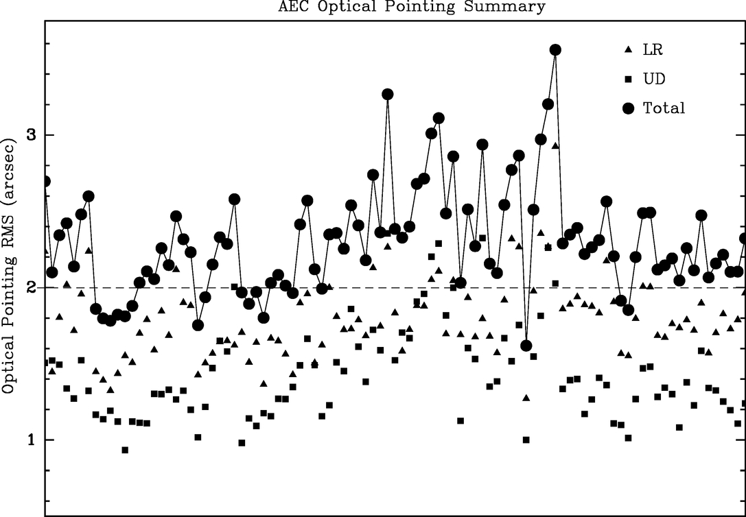
Fig. 19.— AEC antenna OPT all‐sky pointing rms. The horizontal, vertical, and total rms are shown.
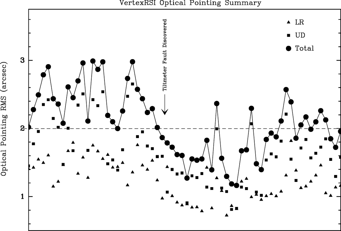
Fig. 20.— Same as Fig. 19, but for the VertexRSI antenna.
6.4. Radiometric Pointing Measurements
Details of the radiometric test procedures can be found in R. Lucas et al. (2004, unpublished).7 The radiometric data were logged in a different way from the OPT data and required some preprocessing, but the end results were similar in the two cases.
6.4.1. Radiometric Pointing Models and Results
Essentially the same procedure was used for both the OPT and the radio data. Special TPOINT scripts were used to mass‐reduce the final selection of files, with automatic removal of outliers and with no manual intervention. The residuals from the different runs were standardized and superimposed, first to look for hitherto undetected terms and then to determine the coefficient values for a fixed "core" group of pointing coefficients.
Radiometric pointing measurements were obtained during the period of 2004 May 16–25 with the AEC antenna and 2004 March 20–22 with the VertexRSI antenna. Some preprocessing of the data was necessary before conventional TPOINT analysis could begin, to fold the operational model back into the observations. Once treated in this way, the four AEC and three VertexRSI measurement runs, which contained 22, 30, 46, and 57 and 44, 48, and 37 pointing measurements, respectively, proved to be sufficiently consistent to simply concatenate them. Fitting each one separately was less promising, given the relatively small number of observations in each data set.
For both antennas, the first model tried was the OPT model, in which only IE, CA, and HECE were allowed to vary. The first and second terms are simply the radio boresight offset relative to that of the OPT. The third term is the Hooke's law vertical flexure, which will be different for the radio and OPT cases. With this approach, the residuals were clearly systematic.
To deal with the elevation errors as a function of elevation, both HESE (elevation errors proportional to sin E) and TX (elevation errors proportional to tan Z) were tried, and the former worked best. This suggested some asymmetry in the BUS, subreflector supports, or nutator.
There were also signs that the azimuth zero‐point correction (IA) and/or the az‐el nonperpendicularity (NPAE) had changed. The explanation (see § 6.4.2) seems to be that the asymmetric location of the OPT, mainly in the horizontal direction, makes it vulnerable to elevation‐dependent flexures in the BUS, a sideways deflection of the OPT occurring as the BUS "opens out" with increasing elevation. It was therefore decided to allow both of these terms to vary, in addition to CA. For the AEC antenna, these tests showed that a substantial 15'' change in IA was needed, as well as an additional core term (HESE), but with no significant change in NPAE (under 1'', in fact). For the VertexRSI antenna, only an 8'' change in IA was needed, but large changes in HESE (46'') and NPAE (27'') were required.
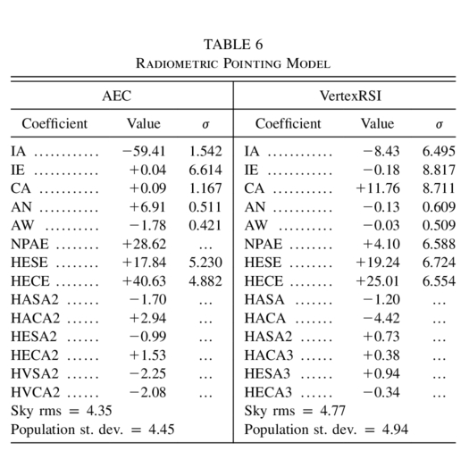
By allowing IA, IE, HESE, HECE, and CA to vary for both antennas (and for good measure, AN and AW; these may change slightly, depending on static wind pressure, and as they are rather uncorrelated with other terms, they are safe to include), satisfactorily nonsystematic residuals were obtained. The final model that was obtained for both prototype antennas using this procedure is listed in Table 6.
 |
For both antennas, a plot of the ΔAcos E and ΔE errors against observation number shows evidence of drifts during each of the pointing runs. For the VertexRSI antenna, the average drift for each of the three runs was just under 02 per observation. If the data from the three VertexRSI radiometric pointing runs are simply concatenated, without individual boresight adjustments, drifts in both ΔAcos E and ΔE can be seen.
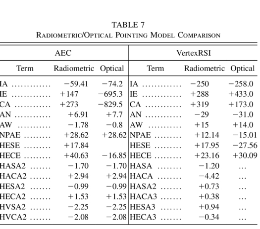
To derive the "best radiometric pointing model" from these measurements without any drift corrections, we used an analysis procedure similar to that used for the optical pointing measurement reductions. The HESE, HECE, and NPAE coefficients were iteratively refined, and the individual pointing runs were normalized by freeing them from their preferred IE, CA, AN, and AW values. The normalized data were then combined and fitted for the five AEC and four VertexRSI core terms, plus IA, HESE, and HECE (and NPAE for the VertexRSI antenna). The resulting "best radiometric pointing models" for the AEC and VertexRSI antennas are shown in Table 7.
 |
The model for each antenna was applied individually to each run by fitting only IE (plus drift), CA (plus drift), AN, and AW, and the results were combined (Fig. 21). The overall 32 and 53 rms figures for the AEC and VertexRSI antennas, respectively, should be treated with some caution: superimposing individually fitted runs is a particularly optimistic way to present pointing results.
An analysis of the same 3 days of data was done (R. Lucas et al. 2004; see footnote 7) using the Plateau de Bure pointing model software. The results are in full agreement. No systematic effect was detected: the results are dominated by measurement errors.
6.4.2. Optical/Radiometric Pointing Correspondence
The location of the OPT within the backup structure of the antenna requires that one consider how the measurement axes of both systems are related. In the pointing model for the antenna concerned, for an ideal OPT fixed to the radio telescope surface and assuming mechanical symmetry about the axis of the parabola, one would expect only the boresight offset (IE and CA) and vertical flexure (HECE) terms in the pointing model to change. However, on both antennas, preliminary analysis of the radiometric pointing showed signs of changes in the azimuth zero‐point correction (IA) and/or the az‐el nonperpendicularity (NPAE). The likely explanation of such effects is that the asymmetric location of the OPT, mainly in the horizontal direction, makes it vulnerable to elevation‐dependent flexures in the BUS, a sideways deflection of the OPT occurring as the BUS "opens out" with increasing elevation. A deflection proportional to sin E would produce a term that is functionally identical to NPAE, while the cos E phase would produce an apparent change in IA.
For a perfect parabola at an elevation of 45°, the aperture of the antenna will become more elongated in azimuth at the zenith and more elongated in elevation at the horizon. Since the ALMA OPTs are located azimuthally off‐axis, the boresights of the OPTs are expected to be pointed to more positive azimuths at the zenith and to more negative azimuths at the horizon. One would expect then the following additional harmonic elevation and azimuth terms to the OPT pointing correction with respect to the radiometric pointing model:
This indicates that one should expect fixed differences between the radiometric and optical determinations for IA, NPAE, HESE, and HECE.
Taking the VertexRSI antenna as an example, a mechanical verification of this theory can be derived from the measured axial focus change due to BUS deflection (see Greve & Mangum 2006). The VertexRSI BUS axial focus is measured to deflect by +1.7 mm over an elevation range of 0°–90°. Using an 80% radiometric taper leads to a deflection of +1.35 mm. With the constants
we find that for a perfect parabola,
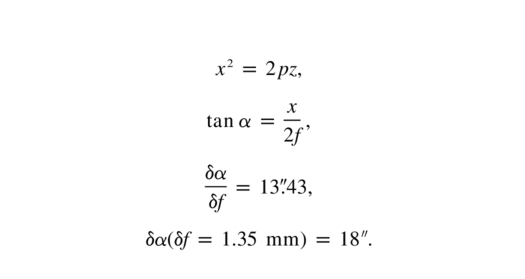
This corresponds well to the combined measured shift in NPAE (+24'') and IA (−7'') between our optical and radiometric pointing models for the VertexRSI antenna.
6.4.3. Radiometric Seeing
We have investigated the influence of refractive pointing errors, or "radiometric seeing," on our radiometric tracking measurements. Measurements of the differences between radiometrically derived positions and their corresponding encoder positions while tracking a source for 15–20 minutes strongly indicate the existence of a refractive pointing error term (see M. Holdaway et al. 2006, in preparation). These refractive fluctuations result in an ∼06 radiometric positioning jitter. The magnitude of the inferred atmospheric pointing structure function at 1 s (the atmospheric crossing time of a 12 m antenna) is predicted to within 10% by theoretical arguments about refractive pointing jitter and atmospheric phase interferometer data.
6.5. Optical Offset Pointing Tests
To investigate the accuracy of the offsetting performance, OPT observations were made in which the antennas were switched repeatedly between a number of stars over distances of about 2°. Four AEC and seven VertexRSI runs were conducted in this manner, consisting of two to five and three to seven stars, respectively. The analysis of these observing runs proceeded as follows:
- 1.Fit and remove the standard 13 parameter pointing model. In this model, all parameters except the boresight offsets IE and CA were held fixed.
- 2.Remove outliers.
- 3.Concatenate the resulting files and perform a final fit to a model consisting only of the boresight position and drift terms IE, CA, A1S, and A1E. This exhaustive removal of position and drift effects is appropriate here, because we are investigating neither tracking nor all‐sky pointing. The individual stars in the field are all equally affected by these measures, with any systematic effects associated with the transition from one star to another left as a residual.
- 4.For each star in this concatenated data set, fit a model consisting of IE and CA alone. This last step reveals any systematic offsetting errors.
The displacements of each star from the mean were then examined. Figure 22 shows sample offset pointing residuals resulting from these analyses for each antenna. The majority of the offset optical pointing runs for both antennas resulted in a derived offset pointing performance within the 06 specification. A couple of these optical pointing runs resulted in offset pointing residuals in the 09–11 range. These results appear to show that both antennas just miss the 06 offsetting specification. However, it must be borne in mind that not only were the experiments delicate and vulnerable to many sources of error, but also that the results were achieved without the metrology systems being active.
6.6. Metrology Performance
The AEC prototype metrology system was originally composed of three components:
- 1.Temperature sensor system to measure the pointing offsets due to thermal deformation of the structure.
- 2.Tiltmeter system to measure pointing offsets due to tilts in specific structural elements.
- 3.Laser interferometer system to measure structural changes in the fork arms of the antenna.
Only the temperature sensor and tiltmeter systems were installed on the prototype antenna. Attempts by AEC to qualify the temperature sensor and tiltmeter metrology systems were unsuccessful. The limited number of measurements that the AEG made while these metrology systems were active led to a poorer pointing performance for the antenna, which is a clear indication that these metrology systems were not functioning properly.
The VertexRSI antenna was designed to meet the pointing specifications with the aid of two separate metrology systems:
- 1.A displacement sensor system mounted on the CFRP reference structure near each elevation encoder. This system was designed to measure the tilt component of the fork arm structure and BUS, which cannot be measured by the encoders themselves.
- 2.A system composed of two tiltmeters in the pedestal of the antenna. These tiltmeters are designed to measure the tilt of the azimuth axis.
Well into the evaluation, the tiltmeter metrology system readout was found to drift by many tens of arcseconds over timescales of up to 1 minute. It was not clear what was causing these drifts. This could be due to a problem with the software that applies these tiltmeter measurements to the antenna positioning, or to a mechanical problem with the mounting of the tiltmeters themselves. Once this problem was discovered, all pointing measurements were made with this metrology system disabled.
A number of measurements were made that included the corrections applied by the displacement sensor metrology system. Unfortunately, these measurements were not extensive enough to evaluate the effectiveness of the displacement metrology system. At the very least, this system did not make the pointing performance of the VertexRSI antenna worse.
We should note that even though none of the delivered metrology systems appeared to improve the pointing performance of either antenna, both antennas met the ALMA pointing specifications. Apparently, the antennas alone outperform their designed pointing performance specifications.
6.7. Evidence of Tripod Print‐Through on the VertexRSI Antenna
To assess the viability of the low‐level (≲1'') terms in our pointing models, we have checked the physical association of two of these minor terms with a plausible mechanical deformation on the VertexRSI antenna. The portion of the OPT pointing model involving HESA3 = +0.94 and HECA3 = −0.34 shows that the antenna nods in elevation as it rotates in azimuth, executing three cycles of nodding per turn of azimuth. This may be evidence of print‐through from the tripod support into the azimuth bearing. The effect can be illustrated by removing all but those two fixed terms from the model and then applying the model to a grid of stars all over the sky. The resulting plot of elevation corrections versus azimuth is shown in Figure 23.
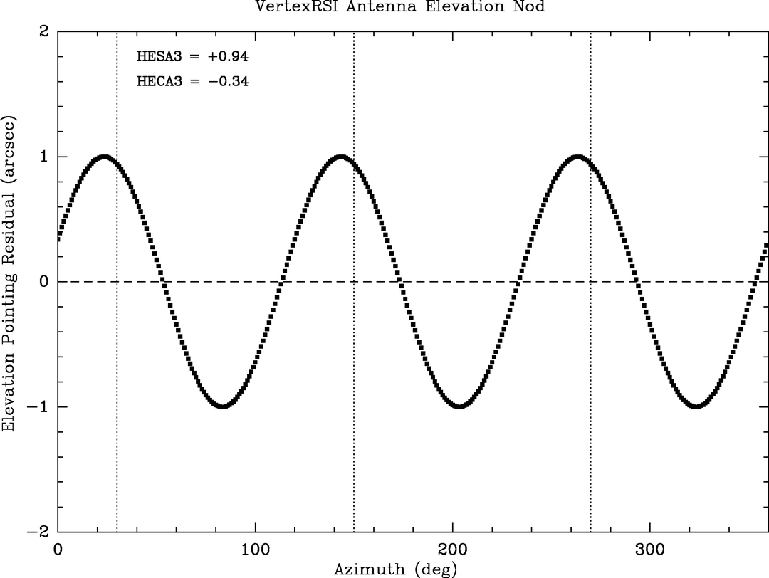
Fig. 23.— HESA3 and HECA3 pointing model terms showing possible tripod print‐through in the azimuth motion of the antenna. The azimuth positions of the three mount points of the VertexRSI antenna are shown as dotted vertical lines.
The azimuths of the three pedestal legs would be aligned to the maxima of the nodding if there were no HECA3 term. The misalignment to the tripod leg positions is arctan (0.34/0.94)/3, or about 7°. The sign of the correction is such that when the antenna is pointing over a pedestal leg, the star is about 1'' higher in the sky than indicated by the elevation encoder reading.
To further confirm the mechanical interpretation of this sin 3A pointing term, measurements with the tiltmeter installed above the azimuth bearing were made at a slow speed (01 s−1) and ±260° rotation in azimuth. These measurements show a single‐angular sinusoidal response (sin A) due to the inclination of the azimuth axis, and a triple‐angular sinusoidal response (sin 3A) due to a repeatable wobble in the inclination of the antenna. The triple‐angular wobble is attributed to a wobble of the azimuth bearing and amounts to ±15; the extrema of the wobble are correlated with the location of the three‐corner support of the pedestal. After elimination of the components sin A and sin 3A, the residual deviation amounts to less than ±05 (peak to peak).
The location of the extrema of the residuals from the sin A + sin 3A fit is further evidence that the triple‐angular wobble is a print‐through of the pedestal mount. The best‐fit values to the measurement given by
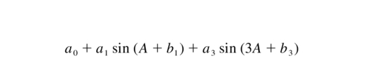
are listed in Table 8 and shown in Figure 24.
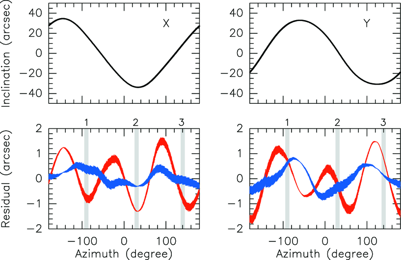
Fig. 24.— VertexRSI antenna measurement of −180° to +180° azimuth rotation. The left column is the x‐direction of the tiltmeter, and the right column is the y‐direction. The red curves are the residuals of the best‐fit a0 + a1sin (A + b1), and the blue curves are the residuals of the best‐fit a0 + a1sin (A + b1) + a3sin (3A + b3). The gray lines show the location of the pedestal corners (1, 2, 3).
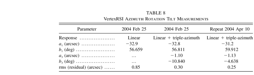 |
We conclude that the telescope/azimuth bearing has a triple‐azimuth wobble that seems to be very stable and that is recovered and corrected for in the pointing model. The location of the triple‐azimuth term suggests a print‐through of the pedestal mount.
6.8. Accelerometer Measurements of Pointing Performance
The accelerometer system described in § 5.3 and Snel et al. (2006) was used to derive three components of the antenna pointing performance:
- 1.Cross‐elevation pointing (left and right accelerometers on the rim of the BUS).
- 2.Elevation pointing (top and bottom accelerometers on the rim of the BUS).
- 3.Subreflector structure translations with respect to the BUS (four accelerometers on the rim of the BUS and one on the receiver flange).
In the following, we characterize antenna pointing performance during several operational modes:
- 1.Pointing toward a fixed (az‐el) without tracking (called "stationary pointing"). In this mode, the drives are powered and the brakes are released. Wind effects are optimally investigated in this mode, as any effects of antenna shake due to position updates are minimal.
- 2.Sidereal tracking. During sidereal tracking, the antenna drives are constantly updating the azimuth and elevation positions, including the azimuth and elevation speed, in order to achieve a smooth tracking motion. Sidereal tracking was checked for 30 azimuth/elevation combinations spread evenly over the sky. Calm wind conditions were chosen in order to clearly separate effects due to the drive system from those due to wind.
- 3.Interferometric mosaicking and OTF mapping at 005 and 05 s−1 scan speeds, respectively.
During the accelerometer measurements, simultaneous wind speed and direction measurements were used to eliminate the effects of the local wind spectrum. Wind‐related antenna performance was calculated for the same wind spectrum that was used for the design of the antennas. Our measurements provide us with the structural stiffness for wind excitation at frequencies between 0.1 and 3 Hz. We extrapolate from these to lower frequencies, using the low‐frequency component of the specified wind power spectrum to predict the pointing jitter due to wind for timescales up to 15 minutes (0.001 Hz). Because we could not measure the tracking jitter at these low frequencies, a conservative value equal to the observed tracking jitter at 0.1 Hz was used at 0.001 Hz as well.
The measured pointing errors under the various measurement conditions are assembled in Table 9. The cumulative errors as a function of frequency are shown in Figure 25 for the case of maximum wind (9 m s−1) and are scaled to the atmospheric situation at the final ALMA site at 5000 m altitude. The section of the curves below the frequency of the asterisk has been extrapolated with the estimated constant value of the stiffness transfer function, as explained above. Figure 26 shows a similar plot for the pointing jitter during sidereal tracking and low wind.
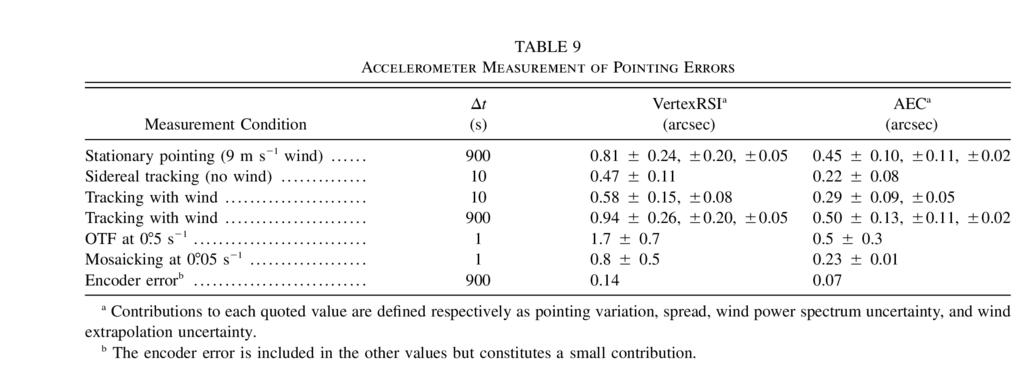 |
To supplement the information summarized in Table 9, we note that
- 1.For stationary pointing conditions under high wind loads, the BUS rim wind shake is dominated by elevation motion for both antennas.
- 2.For sidereal tracking during low wind conditions, the tracking jitter of both antennas is largely due to elevation motion, with large contribution in the 3–6 Hz range. The largest jitter is observed for low elevation, while minimum tracking jitter is seen while crossing the meridian.
- 3.Assuming that the pointing jitter due to wind and that due to sidereal tracking are uncorrelated allows for the determination of the cumulative pointing error. A check of an independent measurement with high wind and sidereal tracking shows that this assumption is valid. Since no tracking jitter at 0.001 Hz can be measured, a conservative value equal to the observed tracking jitter at 0.1 Hz is used.
- 4.For the VertexRSI BUS pointing stability during the fast (05 s−1) OTF scan, the azimuth and elevation at which the scan is performed have large impact on the pointing stability during the scan, which is reflected in the standard deviation given.
- 5.For the AEC BUS pointing stability during the fast (05 s−1) OTF scan, pointing is affected for some parts of the scan by apex rotation feeding back to the BUS motion. This effect died out after a minute. The spread of 03 (1 σ) reflects this variable pointing stability.
- 6.The contribution of subreflector motion to the total pointing error has been investigated but not included in the results presented here. This anomalous subreflector motion is due to excessive and off‐axis rotation of the AEC antenna apex structure. Our accelerometer system measured only 3 degrees of apex motion, which did not allow for the separation of subreflector translation (which directly affects pointing) and subreflector on‐axis rotation (which has no impact on pointing). The results presented here are for BUS pointing only.
We would like to note that measurements of the dynamical behavior of the antenna under operational conditions at this level of accuracy are extremely hard to perform radiometrically. The use of accelerometers for this purpose provides accurate results quickly and might be considered for routine checking of pointing stability.
6.8.1. Pointing Effects Due to Apex Motion
The apex structures of both antennas rotate about an axis that is assumed to be aligned with the boresight axis. However, for the AEC antenna, this axis is offset by −1.5 to +1.0 cm, depending on the elevation. Fast switching can excite the rotation mode, which has translation components on‐axis that can amount to 30 μm peak to peak. The rotation and corresponding translation component is at 5 Hz and damps out with a 1/e decay time of 5 s. With the prime‐focus plate scale of 34'' mm−1, this translates to radio pointing errors of up to 1'' peak to peak in cross‐elevation, provided that the rotation axis is parallel to the boresight axis, which could not be confirmed with the equipment available.
For the VertexRSI antenna, minor apex structure rotation was observed, which did not affect antenna performance, since the rotation appears to be on‐axis.
6.9. Pointing Performance Summary
- 1.Due to the remarkably good pointing performance of both antennas, neither the optical nor radiometric tests offer sufficient resolution to tie down the performance of either antenna definitively, especially in the area of offset pointing.
- 2.The metrology systems were never properly commissioned and in most cases did not appear to work properly.
- 3.For the AEC antenna, the all‐sky pointing is just outside specification, typically 22 rms but with occasional 2'' rms results. The cross‐elevation residuals were usually slightly larger than the elevation residuals, especially earlier in the test period, when the elevation performance was particularly good. A sequential multiple star measurement was used to estimate the seeing and short‐timescale antenna positioning errors. These measurements suggest a seeing/vibration contribution of ∼15, in line with the results from radiometric tracking tests (M. Holdaway et al. 2004; see footnote 3). Extending the interpretation to account for the seeing contribution suggests that the true antenna pointing residual is 17. This result should be weighed against the rather optimistic approach to the analysis presented in this document.
- 4.For the VertexRSI antenna, the all‐sky pointing performance was typically 15 rms.
- 5.The pointing model appears to be quite stable (exceptionally so in the case of the azimuth axis tilt terms) on the AEC antenna. Pointing model stability was measured to be adequate on the VertexRSI antenna. These measurements suggest that during operational use, recalibration of each antenna (using perhaps four stars around the horizon and one near the zenith) every couple of hours would maintain peak pointing performance.
- 6.The offsetting performance of both antennas sometimes appeared to fall just short of the 06 rms specification for offsets of 2° or less, but this is a tentative result and is not seen in all test runs. Given that the very stringent antenna specifications are a challenge that the measuring techniques struggle to meet, and taking into account the fact that the results were achieved without the help of the metrology systems, it is perhaps wise to return an open verdict on this aspect of the performance of the ALMA prototype antennas.
- 7.Using the accelerometers, the implied requirement of 06 tracking stability in the offset pointing specification could be checked for sidereal tracking and wind shake. The VertexRSI antenna marginally misses this specification (094 rms pointing stability over 15 minutes), while the AEC antenna was measured to be more stable at 050 rms.
- 8.The wind‐induced pointing jitter over timescales up to 15 minutes at wind speeds of 9 m s−1 was calculated in the antenna error budgets to be 0035 (VertexRSI) and 035 (AEC) rms. The accelerometers measured these values to be 081 (VertexRSI) and 045 (AEC) rms, excluding the effects of subreflector motion.
- 9.OTF scanning at 05 s−1 led to an average pointing stability over timescales of 1 s that amounted to 17 rms for the VertexRSI antenna and 05 rms for the AEC antenna. The specification is that the position is known at a given time, but the antenna does not need to point at the commanded position at that time. Measurements confirm that the pointing jitter as seen by the encoders matches that derived from the accelerometers.
- 10.During interferometric mosaicking with rates of 005 s−1, the commanded path is followed within 08 rms for the VertexRSI antenna and 023 rms for the AEC antenna. These are well within the specified value of 1'' rms.
- 11.The radiometric tests are too few for any firm conclusions to be drawn. At the frequency used, the beam width is about 1' FWHM, and the rms result is less than 10% of this, so there is no reason to suppose the underlying pointing and offsetting accuracy is poorer than the OPT measurements suggest.
7. FAST SWITCHING
7.1. Optical Pointing Telescope Measurements of Fast‐switching Performance
OPT offset and encoder data were used to compare the fast‐switching capabilities of the VertexRSI and AEC antennas. These fast‐switching measurements are performed by position switching between two stars that are bright enough to get high signal‐to‐noise ratio (S/N) position fits at the highest possible position‐switching rate (about 0.1 Hz). The optical pointing offsets as a function of time for each slew tell us how quickly the antenna can get on‐source and how quickly the pointing settles down after it gets on‐source. The optical pointing offsets include both mechanical antenna pointing and atmospheric seeing caused by dry air fluctuations (unlike in the radio, where the pointing jitter is caused mainly by water vapor fluctuations). Reasonable evidence that the encoders accurately reflect the antenna's mechanical motion is shown in M. Holdaway et al. (2004; see footnote 3). Hence, we expect that the encoder pointing offsets should also be very useful.
7.1.1. OPT Fast‐switching Measurements
All OPT fast‐switching measurements were made on 2004 April 20. Four different star pairs were observed with each antenna. Two star pairs did not yield valid data for the AEC observations, while all four pairs of stars yielded good data on the VertexRSI antenna. Details of these observations are summarized in Table 10.
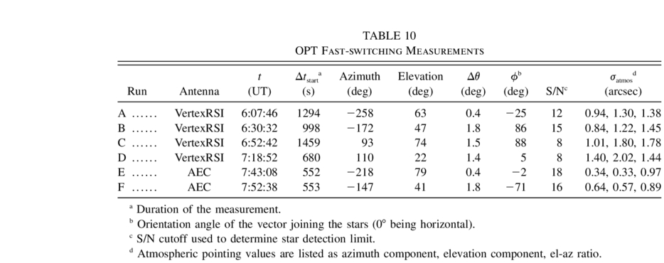 |
For each measurement run, the following analysis was performed:
- 1.The 20 Hz sampled encoder az‐el position information was linearly interpolated to match the corresponding 10 Hz sampled OPT az‐el star position information.
- 2.Positions from the OPT az‐el data stream were identified as "target" (on‐source) and "calibrator" (off‐source) positions by assigning a star S/N cutoff to the OPT measurements.
- 3.Each target‐to‐target observation consumed about 5 and 4 s for the VertexRSI and AEC antenna measurements, respectively. Roughly speaking, the first ∼1.5 s are spent slewing to the source, the next second is spent refining the pointing, and the remaining time has a nearly stable pointing level.
- 4.The constant az‐el offset, representing the antenna pointing model, is removed from the OPT star position fits in order to derive the az‐el offset for each measurement.
- 5.For each run, a single fourth‐order polynomial fit to the azimuth and the elevation encoder readings for the last half of all scans was subtracted from the azimuth and elevation encoder readings for that run in order to derive the rms pointing errors.
- 6.For each slew, we are interested in the rms pointing error as a function of the time since the last measurement from the previous slew. Time bins 0.2 s long (twice the basic data sampling rate), which represents the time from the end of the previous scan and from the rms of the azimuth and elevation offsets that fall into that time bin for all data in a 10–20 minute observation, were constructed.
- 7.Typically, about 2% of the data points in each run were determined to be outliers and were removed.
- 8.Optical rms azimuth offsets, rms elevation offsets, and the total rms optical and encoder pointing errors as a function of time for each run and antenna were then derived. Figure 27 shows these results.
Comparing each run az‐el profile (see Fig. 27), one sees general agreement, indicating that these two data streams are reliably aligned in time. However, the optical pointing rms generally exceeds the encoder rms pointing, as expected, as the optical rms includes the effects of optical seeing. The optical seeing (σatmos) will be uncorrelated with the mechanical pointing errors, so it can be extracted from the optical pointing contribution by a quadratic subtraction:
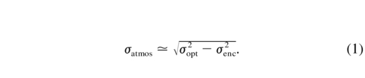
Table 10 shows the inferred atmospheric pointing contribution for each observation. In deriving these data, we considered optical and encoder data past the 2.5 s point in the profiles shown in Figure 27, calculated the inferred atmospheric optical pointing for each time bin, and took the average for all time bins past 2.5 s. Note that for the VertexRSI antenna, the ratio of elevation atmospheric pointing to azimuth atmospheric pointing is greater than 1.0, but for the AEC antenna, it is about 1.0. We suspect that this is a further indication of the poorer elevation (VertexRSI) and azimuth (AEC) tracking and pointing performance noted in § 6.
In conclusion, we find the following from our OPT measurements of fast‐switching performance:
- 1.The VertexRSI antenna typically reaches its target source in 1.5–2.0 s.
- 2.The VertexRSI antenna can have a significant pointing bounce in elevation between 2 and 3 s after the slew begins. Presumably, the servo is not well tuned, and this is a correction for overshooting or something similar.
- 3.The AEC antenna arrives at the target source after about 1.5 s and has a much smaller pointing error after acquiring the source.
- 4.The VertexRSI antenna has larger pointing errors than the AEC after the source has been reached, although the encoder data indicate that the specification of 06 is approximately met.
7.2. Radiometric Fast‐switching Measurements
We simulated radiometric fast‐switching interferometric observations by a repetitive measurement sequence consisting of a blank‐sky integration, slew, then target‐source integration. The blank‐sky integration simulates a fast‐switching calibrator measurement. The detailed sequence of measurements was as follows:
- 1.In order to see pointing fluctuations in both azimuth and elevation, we performed observations with Jupiter at both its azimuth and elevation half‐power points (Table 11) and with a sequence of 21 antenna slews to the nearby "calibrator" (i.e., blank sky) of 15 in both azimuth and elevation.
- 2.These total power measurements utilized beam switching to eliminate variable atmospheric emission with a subreflector throw of about 80'' nutating at 10 Hz. The resulting differential total power measurements were found to be limited by gain fluctuations in our radiometric receiver system rather than incorrect cancellation of the atmospheric emission or thermal noise.
 |
In summary, the analysis of these measurements proceeded as follows:
- 1.To calibrate the conversion from total power level to source offset, we collected a series of three beam‐switched total power measurements at offsets of +35'', +40'', and +45'' from the half‐power point of Jupiter. These data indicate that the total power should change by about 0.160 for every arcsecond of pointing offset in the direction of the offset. In the following, we adopt this value for the change in total power versus position. The true scaling factor will be very close to this for the elevation scans, but the azimuth scans could have a scaling factor significantly different from this (i.e., as low as 0.11), which will increase the radiometrically inferred azimuth errors by as much as 50%, due to uncertainties in the interpretation of the unmeasured peak flux for Jupiter. Note that the rms of the 0.1 s data samples when off‐Jupiter were typically 0.033. At 0.160 arcsec−1, this indicates that the radiometer noise is equivalent to a jitter of 021. Averaging for longer times can give us estimates of pointing errors with smaller uncertainties.
- 2.For each 0.1 s time stamp since the start of a slew (there are 20 slewing profiles going toward Jupiter per scan), we calculate the rms of the measured total power minus the mean total power calculated from the last half of all 20 blocks in the scan, and divide by our calibration factor of 0.16 amplitudes arcsec−1. All 20 slew profiles within a given scan are then aligned and averaged to derive the radiometrically inferred pointing error as a function of time, all shifted so they align with the slew that got on‐source fastest. A representative sample of these results is shown in Figure 28.
- 3.By averaging the approximately 500 samples made during the last half of each scan, a measure of the radiometric tracking accuracy, which includes contributions from the antenna and atmospheric fluctuations, was derived for the VertexRSI antenna. Typical values of 06 per axis, or about 08 total, were measured.
- 4.In the AEC antenna measurements, we note that there is a 5 Hz oscillation in the positioning. This is a real mechanical effect because
- a)It has too much power at too small of a timescale to fit with the atmospheric pointing error structure function.
- b)It is seen in the encoder data (offset by 0.1 s).
- c)It is not seen in the tracking data.
- d)It seems to get excited as the telescope stops, and dies down with time (i.e., the telescope is settling down).
4. This oscillation has been identified as being due to a mechanical oscillation of the apex structure (Snel et al. 2006).
7.2.1. Radiometric Fast‐switching Performance Conclusions
Using radiometric and encoder data, we have investigated the mechanical aspects of the fast‐switching performance of the ALMA prototype antennas.
- 1.The VertexRSI antenna basically meets the fast‐switching specification of "1.5 degrees in 1.5 seconds to an accuracy of 3 arcseconds." The antenna achieves pointing errors of about 08 rms if a bit more settle time is permitted. Minor improvements in the software and servo systems could improve the fast‐switching capability. We find that for nighttime observing, the encoders and the radiometrically inferred pointing errors agree remarkably well. After the slew has been completed and the antenna is pointing on‐source, pointing drifts of under 1'' over 2 s of time, and pointing jitter of amplitude 03 and frequency 3 Hz, can be seen clearly in both the encoder pointing and the radiometrically inferred pointing. On average, the encoders and radiometrically determined pointing differs by 028 rms while slewing, and 015 after settling.
- 2.Radiometric and encoder data from the AEC prototype antenna indicate that the AEC antenna meets the fast‐switching motion requirements. We see that as the AEC antenna comes to rest after a fast slew, a 5 Hz oscillation is excited by the fast‐switching motion, and that the peak amplitude of this oscillation is about 04, which dies out over a few seconds. Accelerometer measurements have identified this oscillation as being due to a rotation of the apex structure (Snel et al. 2006). For the measurements performed in this report, this oscillation does not prevent the AEC antenna from meeting the fast‐switching specification.
7.3. Encoder Measurements of Fast Motion and Settling Time
From comparisons of the accelerometer measurements to the antenna encoder position information, we gain an insight into the settling time after the fast position switch. We find that the VertexRSI antenna can perform a fast switch in the prescribed time and positioning limits, but not for all directions. There are no indications that the AEC antenna does not meet the fast motion and settling time specifications.
8. PATH‐LENGTH STABILITY
The path‐length stability of the antenna structures was measured using an Automated Precision, Incorporated, (API) 5D (5 degrees of freedom) laser interferometer (Greve & Mangum 2006) and an accelerometer system (Snel et al. 2006). In the following section, we describe the path‐length stability measurement results for both prototype antennas. Detailed descriptions of the technical capabilities of each measurement system are given in the associated references.
8.1. API5D Laser Interferometer Measurements
An API 5D (API5D) laser interferometer was used to measure the individual structural components that comprise the total interferometric path length through the antennas. Laser interferometers are used to measure variations in "straightness" along a given path. One component of this "straightness" is the path‐length variation, Δz. For the measurements made of the ALMA prototype antennas, the accuracy in Δz is better than 1 μm for an enclosed path and 2–3 μm for an open‐air path.
Since the total path‐length variation cannot be made with a single measurement, the total path length was separated into four parts (pedestal, fork arm, central receiver flange to subreflector, and subreflector to surface) and measured during a representative sample of observing conditions and operation modes. As shown in Figure 29, these measurements contain the following:
- 1.L1.—Path length inside the pedestal: distance between the foundation (ground) and the lower face of the azimuth bearing. It was not possible to measure this path length on the AEC antenna.
- 2.L2.—Path length inside (one) fork arm (left, right): distance between the lower part of the traverse and the upper part of the (left, right) fork arm, below the elevation bearing.
- 3.L3.—Path length along the radio axis: distance between the upper part of the Invar cone (VertexRSI) or the vertex hole (AEC, laser tracker mount) of the main reflector and the apex of the subreflector. In the measurements, the dilatation of the aluminum subreflector support tube (50 cm length) has been eliminated as far as possible.
- 4.L4.—Path length of the reflector: distance between the Invar cone/vertex hole and a point of the reflector surface, measured via the subreflector. On both antennas, this path‐length measurement was tested but not routinely performed, mainly because of difficult alignment and time limitations. Since in essence this path‐length component originates in the CFRP part of the antennas, any temperature‐induced path‐length variation is expected to be small.
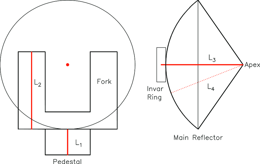
Fig. 29.— Illustration of the path‐length measurement scheme. Red lines indicate the path‐length sections measured with the API laser interferometer system.
The full path‐length variation is approximately the sum of the measured components. Table 12 and Figure 30 present the results from these path‐length stability measurements for both ALMA prototype antennas.
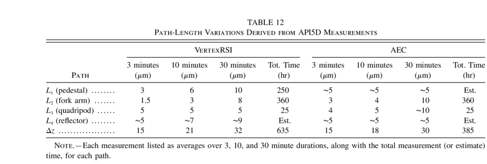 |
From simple geometric and material arguments (thermal expansion coefficients) and the fact that wind forces act on short timescales, it was evident from the beginning that the path‐length changes are primarily due to thermal dilatation of the antenna components, induced by variation of the ambient air temperature and solar radiation and buffered by the surface finish (paint) and thermal insulation. In the analysis of path‐length variations, we have selected several time intervals (Δt): 3 minutes, comparable to the timescale of wind; 10 minutes, comparable to FSW (fast switch) and OTF modes of observation; and 30 minutes, comparable to the time between upgrades of the pointing and interferometer phases. The data shown in Figure 30 were obtained during long time periods (listed in Table 12) and cover a large variety of antenna motions. For path lengths that could not be measured, an estimated value is entered in Table 12.
In the following, we investigate the path‐length dependence of both prototype antennas under a variety of the individual load conditions that went into the overall performance quoted above.
8.1.1. Path‐Length Variations Influenced by Temperature and Wind
For purposes of path‐length prediction, we have searched for correlations of the path‐length changes with the steel temperature of the pedestal and the fork arms, the ambient air temperature, and the wind speed. The correlation of the fork arm path‐length change ΔL2 is shown for the VertexRSI and AEC antennas in Figures 31 and 32, respectively. As expected, the correlation of ΔL2 with the change of the fork arm steel temperature is good and usable for prediction. On the VertexRSI antenna, a similarly useful correlation was found for the path‐length of the pedestal (L1; Greve & Mangum 2006). There is no correlation between path‐length variation and ambient air temperature or wind speed variation.
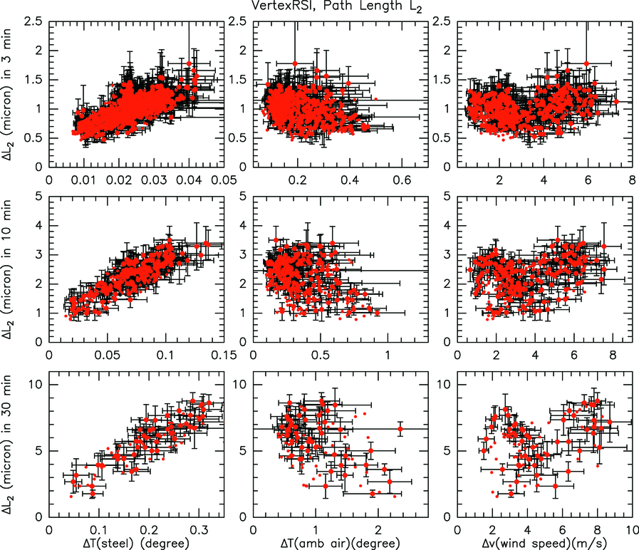
Fig. 31.— VertexRSI antenna dependence of ΔL2 on the temperature variation of the fork [ΔT(steel); left] and ambient air [ΔT(amb air); center] and the variation of the wind speed (Δv; right) for time intervals of 3, 10, and 30 minutes (top to bottom).
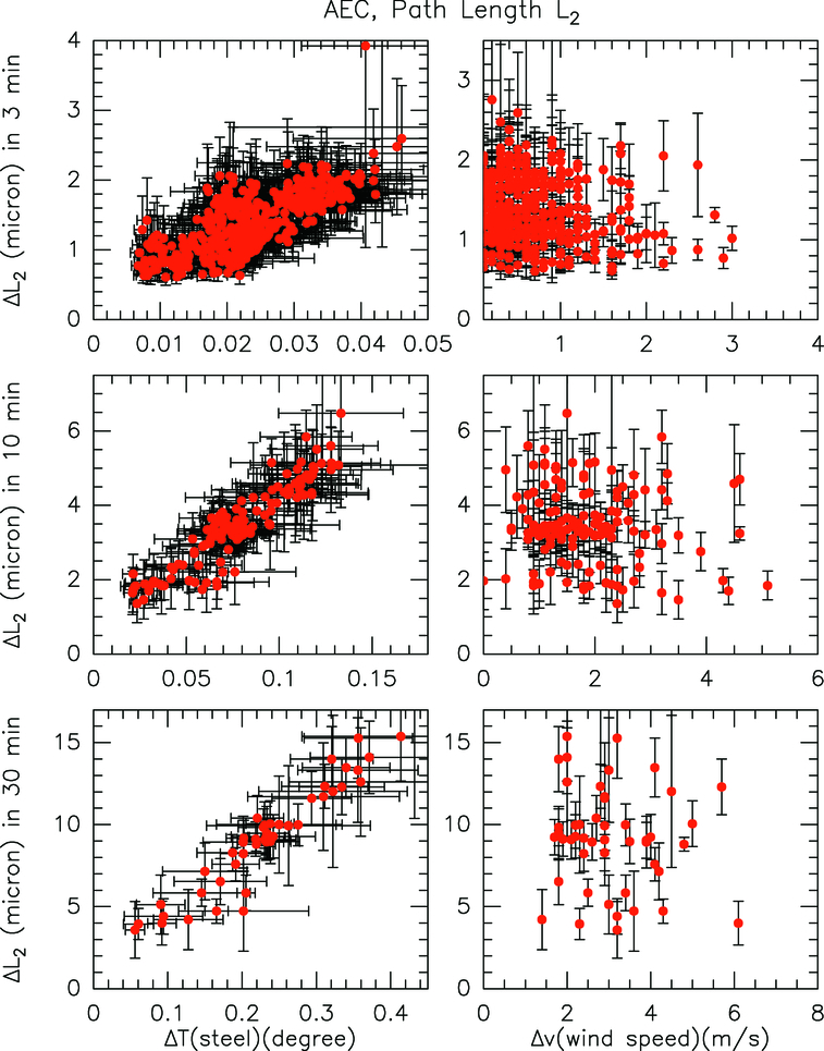
Fig. 32.— Same as Fig. 31, but for the AEC antenna. Measurements of the ambient air temperature were not available.
A dedicated investigation of the path‐length changes with variations in wind speed was difficult, due to logistical reasons. For one particular day with changes of the wind speed (v) from ∼5 to ∼15 m s−1, the path‐length variation ΔL2 (fork arm) of the VertexRSI antenna was measured, and it hinted at a slight increase in ΔL2 with increasing wind speed. However, the measured variation of L2 remained within the specification, even for the highest observational wind speed of v = 9 m s−1. There are no data for the AEC antenna.
8.1.2. Path‐Length Predictions from Steel Temperature Measurements
Both prototype antennas have temperature sensors installed on the steel walls inside the fork arms. From these recordings, we have derived the average, maximum, and minimum temperature of each fork arm. The average temperature distribution measured throughout a fork arm was used in a finite element model (FEM) analysis to calculate the corresponding thermal dilatation ΔL2. Comparing the calculated thermal dilatation with the path‐length variation measured directly with the API5D, we find very good agreement, as shown in Figure 33. From this, we conclude that the path‐length variations of the steel parts can be predicted to a high degree of accuracy from representative temperature measurements used in the FEM, or from an empirical relation.
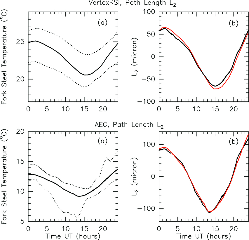
Fig. 33.— Correlation between the path‐length variation ΔL2 measured with the API laser interferometer and FEM‐calculated path length derived from the measured fork arm temperatures (14 sensors) for both prototype antennas. (a) Average (solid line) and maximum and minimum temperatures (dashed lines) of the fork arm steel derived from 14 sensors. (b) Measured path‐length variation (black line), and that calculated from the FEM using the average temperature (red line). Similar results were obtained for other days.
The daily temperature variation of the fork arms and the corresponding path‐length variation ΔL2, both shown in Figure 33, can be approximated with good accuracy by sine functions. This holds also for the ambient air temperature, at least as measured at the VLA site during most of the tests. When adopting a sine function L2(t) = L0 + ΔL2sin (ωt), where ω = 2π per 24 hr and t = time, the path‐length variation ΔL2 at a 3, 10, and 30 minute time interval can be derived by differentiation of the function L2(t). The corresponding result is shown by solid lines in Figure 33, which gives an explanation of the double‐peaked form of the measured variations. The minima of ΔL2 occur around 0:00 and 14:00 UT, where the temperature changes of the ambient air and the steel of the fork are smallest.
As is evident from Figure 33, the total daily path‐length variation of the fork arms is of the order of 100–200 μm, as is fully understandable and unavoidable, given the height of the fork arms, the thermal properties of steel, the actual temperature variation of the steel, and the solar illumination.
8.1.3. Path‐Length Variations during Antenna Motion
The ALMA interferometer will use sidereal tracking, OTF mapping, and FSW motions between source and calibrator. The OTF, and in particular the FSW motions, involve high accelerations of the antenna, which may affect the path‐length stability. The path‐length variations ΔL1, ΔL2, and ΔL3 were measured under the following motions of the antennas: (1) sidereal tracking as a combined motion in azimuth and elevation direction, (2) OTF motion of 1° azimuth by 1° elevation at 005 s−1, and (3) FSW motion of 1° azimuth by 1° elevation at 6° s−1 in azimuth and 3° s−1 in elevation.
For both antennas, the variations of the path lengths L1, L2, and L3 are within ±2 μm for sidereal tracking and OTF motion. For FSW motion, with the highest acceleration at the subreflector position of the quadripod, the path‐length measurements L3 are shown in Figure 34. Again, for both antennas, the path‐length variation ΔL3 at the on and off position is within ±3 μm.
8.1.4. Influence of Gravity on L3
Because of gravity‐induced deformations, the path length L3 on both antennas will change with elevation of the reflector. To measure this effect, the laser emitter of the API5D was installed on a mount (one especially constructed for the VertexRSI antenna, but the laser tracker platform on the AEC antenna) at the reflector vertex, and the retroreflector was installed on the subreflector. The measurements of the L3 path‐length variation as function of elevation are reliable, because the measurements are insensitive to a small tilt of the laser mount relative to the antenna structure, and hence of the laser beam reflected in the retroreflector. The antennas were tipped in elevation in steps of 15°, between 5° (AEC) or 15° (VertexRSI) and 90° elevation, and the variation of ΔL3(E) was recorded. These path‐length measurements, along with the path‐length variation predicted from a FEM calculation of the antenna structure, are shown in Figures 35 and 36. The repeatability of the API5D measurements is approximately ±5 μm. Note that in Figure 35, the change in subreflector position as measured by the ALMA Antenna Integrated Product Team using photogrammetry agrees well with the API measurement. Even though there may exist a difference between the measured and calculated variation of L3 with elevation, the results indicate that the variation of ΔL3 must be taken into account in the operation of the interferometer. They are easily put into analytic form.
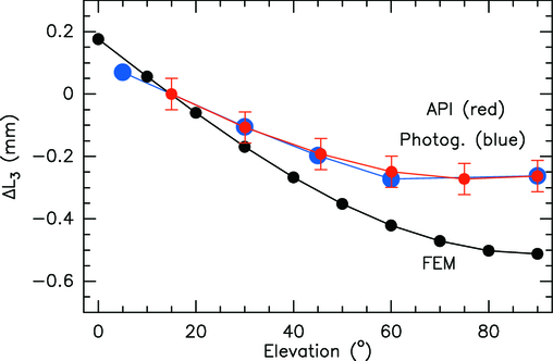
Fig. 35.— VertexRSI antenna path‐length variation ΔL3 as function of elevation of the reflector, measured with the API and by photogrammetry. The curve indicated as FEM is the calculated variation.
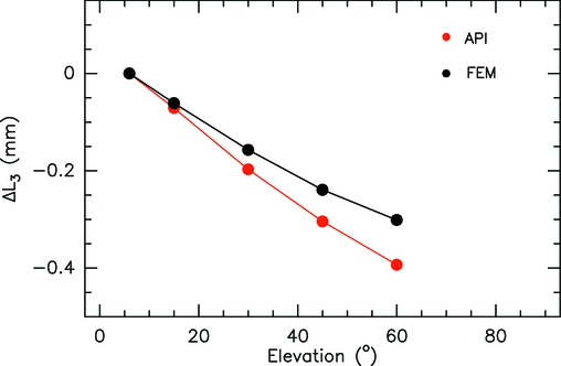
Fig. 36.— AEC antenna path‐length variation ΔL3 as function of elevation of the reflector. The curve indicated as FEM (black) is the calculated variation.
8.2. Accelerometer Measurements of Path‐Length Stability
The accelerometer system described in § 5.3 and Snel et al. (2006) was used to derive the total path‐length stability of the antenna. These measurements were derived from the four accelerometers on the rim of the BUS, one accelerometer on the receiver flange, and an accelerometer on the apex structure. The boresight motion of the BUS is subtracted from twice the boresight motion of the apex structure, which results in the total path‐length variation with respect to ground. As was done for the pointing results derived from accelerometer measurements (see § 6.8), here we characterize antenna path‐length stability performance for the following situations:
- 1.Stationary pointing in high wind.—Wind‐induced total path‐length variations for both antennas amount to 6 μm rms over timescales of 15 minutes. These numbers are consistent with the path‐length stability as determined with the API5D instrument (§ 8.1; Greve & Mangum 2006). For antenna wake conditions, path‐length stability is 11 μm rms over 15 minutes.
- 2.Sidereal tracking.—For sidereal tracking, the total path‐length variations over timescales of 1 s remain below 2 μm for the VertexRSI antenna and below 0.5 μm for the AEC antenna.
- 3.Fast motion.—Total path‐length stability during fast OTF scans with a 05 s−1 scan rate averages to 12 μm rms over timescales of 1 s for the VertexRSI antenna. The AEC antenna path‐length stability averages to 3.3 μm rms. When the scan rate is reduced to 005 s−1 for interferometric mosaicking, total path‐length stability averages to 3.1 μm rms over timescales of 1 s for the VertexRSI antenna, and 0.7 μm rms for the AEC antenna.
9. LIMITATIONS OF THE EVALUATION
In fulfilling its task, the AEG was limited by a number of circumstances. Most importantly, the atmospheric conditions at the VLA site did not allow the antennas to be tested at their highest operating frequencies. It is at the edges of the operational range that the antenna parameters can be most effectively determined by radiometric measurements. This formed the most serious limitation to our evaluation program. Instead, we have employed a number of optical‐mechanical measurement devices in an effort to obtain sufficient material for a valid evaluation of the antennas.
Large delays in the delivery of the antennas shortened the evaluation process and limited the extent to which performance specifications could be tested. The VertexRSI antenna was marginally put at our disposal in 2003 March, and the AEC antenna in 2004 January. Neither antenna was fully functional at those times. Summarizing, our ability to measure the full performance of the prototype antennas was limited in the following areas:
- 1.The holographic surface measurement was limited to one elevation angle. Some data on the reflector surface deformation as a function of elevation were obtained with optical methods.
- 2.The atmospheric conditions at the VLA site are quite different from those at the ALMA site on Chajnantor, Chile. Comparing the temperature and wind variations encountered at the VLA site with those at Chajnantor, it has been possible to draw meaningful conclusions regarding the behavior of the antennas under the conditions specified for Chajnantor. However, at the VLA, the atmospheric transmission only allows observations at the longer millimeter wavelengths and over a limited (winter) period of the year. This has significantly impeded the quantity and quality of the radiometric tests. Moreover, we found that the VLA site has poor seeing, seldom better than 4''. This made the optical measurements of the important tracking and offsetting performance below 1'' difficult to determine.
- 3.Radiometric pointing measurements are the final criterion for the determination of the pointing behavior. The system temperatures of the evaluation receivers are excellent; however, the limits set by gain fluctuations were factors of orders of 20 (at 3 mm) and 10 (at 1 mm) above the thermal fluctuations. Thus, our limiting sensitivity was entirely set by gain stability at the 10 Hz switching frequency, restricting the number of available sources to ∼20 at 3 mm wavelength. The nutator could only operate reliably under quiet or moderately windy conditions (a few m s−1). Only a limited set of data could be collected at the VertexRSI antenna, and even less on the AEC antenna.
- 4.Some specifications fell outside our specific charter, in particular:
- a)Time needed to remove and attach the antenna to its foundation.
- b)Alignment errors after a drop of the antenna during transportation.
- c)Mechanical and electrical requirements.
Considering these circumstances, it is gratifying to report that we were able to collect an amount of data that allows us to draw meaningful conclusions as to the performance of the ALMA prototype antennas. The test program on the VertexRSI antenna began in 2003 March, but really useful data were collected only from 2003 October onward. The AEC antenna program was started in 2004 January. The entire program was concluded by the end of 2004 May. Clearly, this time span did not allow us to make reliable statements on the long‐term behavior of the antennas.
10. CONCLUSIONS
The overall design and performance of the ALMA prototype antennas make either of them an attractive option for a production antenna that will satisfy the stringent ALMA requirements.
The contributions of the following individuals were necessary for the success of the ALMA prototype antenna evaluation process: Marc Rafal (Commonwealth Technical Associates LLC); Fritz Stauffer, Nicholas Emerson, Jinquan Cheng, and Jack Meadows (NRAO); Angel Otárola (ESO); José Lopez‐Perez (OAN); David Smith (MERLAB); Michael Bremer (IRAM); and Henry Matthews (HIA).
Footnotes
- 1
The performance results presented in this publication were part of a comprehensive technical evaluation process used to evaluate the ALMA prototype antennas, which concluded in 2005 April.
- 2
See "Evaluation of the ALMA Prototype Antennas" (J. G. Mangum, J. W. M. Baars, A. Greve, R. Lucas, R. Snel, & P. T. Wallace 2004, ALMA Int. Rep. Coll.).
- 3
See "Evaluation of Fast Switching and Tracking Performance of the VertexRSI and AEC Prototype Antennas Using Radiometric, Encoder, and Optical Data" (M. Holdaway, R. Lucas, & J. G. Mangum 2004, ALMA Prototype Antenna Evaluation Rep. Coll.).
- 4
See "Evaluation of the ALMA Prototype Antennas: Pointing" (P. T. Wallace, J. G. Mangum, & R. Lucas 2004, ALMA Int. Rep. Coll.).
- 5
See "ALMA Test Facility Weather Instrumentation" (J. G. Mangum & A. Greve 2004, ALMA Int. Rep.).
- 6
See "The ALMA Optical Pointing Systems: Design Considerations and Prototype Description" (J. G. Mangum 2004, ALMA Int. Rep.).
- 7
See "Radiometric Measurements of the ALMA Prototype Antennas" (R. Lucas, J. G. Mangum, & H. Matthews 2004, ALMA Prototype Antenna Evaluation Rep. Coll.).