
ABSTRACT
Tennessee State University operates several Automatic Photoelectric Telescopes (APTs) located at Fairborn Observatory in the Patagonia Mountains of southern Arizona. The APTs are dedicated to photometric monitoring programs that would be difficult and expensive to accomplish without the advantages provided by automation. I describe the operation of two of the telescopes (0.75 and 0.80 m APTs) and the quality‐control techniques that result in their routine acquisition of single‐star differential photometry with a precision of 0.001 mag for single observations and 0.0001–0.0002 mag for seasonal means. I show that a primary obstacle to photometry at this level of precision is intrinsic variability in the comparison stars. Finally, I illustrate the capabilities of the APTs with sample results from a program to measure luminosity cycles in Sun‐like stars and a related effort to search for extrasolar planets around these stars.
Export citation and abstract BibTeX RIS
1. INTRODUCTION
For the past decade, the Tennessee State University (TSU) Center of Excellence in Information Systems has been developing the capability to make photometric, spectroscopic, and imaging observations with automatic telescopes. As part of that effort, I have established a program to monitor stellar brightness changes in a variety of stars with automatic photoelectric telescopes (APTs). The APTs are located at Fairborn Observatory's privately owned site near Washington Camp in the Patagonia Mountains of southern Arizona (Fig. 1). Fairborn is a private, nonprofit foundation headed by L. Boyd that has designed, built, and operated automatic telescopes for various institutions for more than 15 years. From early 1986 to mid‐1996, Fairborn was located at the Fred L. Whipple Observatory on Mount Hopkins (see Genet et al. 1987 for an early history) but was relocated to Washington Camp to accommodate its expanding facilities (Eaton, Boyd, & Henry 1996).1
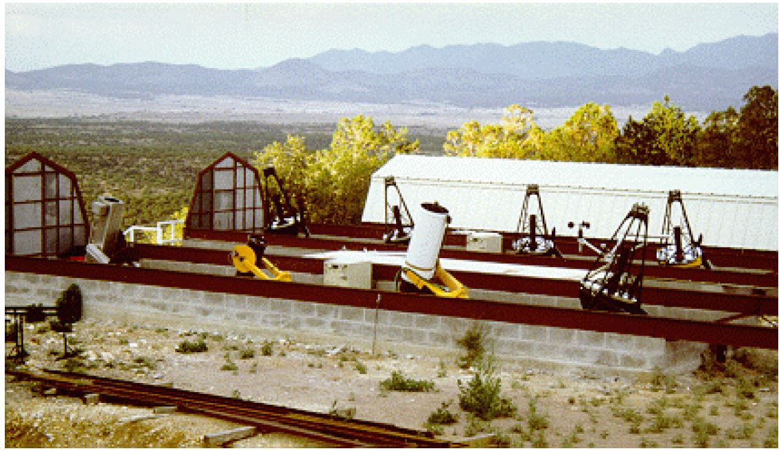
Fig. 1.— The automatic telescope observing site at an altitude of 5700 feet in the Patagonia Mountains of southern Arizona. Currently, eight operating telescopes owned by various institutions are housed in two roll‐off‐roof enclosures (shown in their open positions). The 0.75 and 0.80 m APTs, used to monitor brightness changes in Sun‐like stars and to search for extrasolar planets, are the rightmost two telescopes in the picture. Four additional TSU telescopes (three 0.80 m APTs and a 0.61 m automated imaging telescope [AIT]) are under construction in the third (closed) shelter in the background. TSU's new 2.0 m automatic spectroscopic telescope (AST) (Eaton 1995) is also under construction in its own enclosure nearby.
The telescopes and their photometers operate automatically without human oversight. A site‐control computer, interfaced to a weather station, opens the observatory at the beginning of each night if conditions are suitable and signals the individual telescope‐control computers to begin observing. The site computer monitors weather conditions during the night and directs the observatory to close whenever conditions deteriorate. The telescopes receive their observing instructions over the Internet, and the resulting data are returned automatically each morning.
Several years ago, Young et al. (1991) reviewed the factors limiting the precision of differential stellar photometry and provided a list of 15 recommendations for precision photometry. The APT photometers and observing techniques described in this paper adhere closely to those recommendations, although the use of a special filter set that satisfies the sampling theorem was not adopted since the observing program is restricted to solar‐type stars. The results demonstrate that the automatic telescopes are very effective for carrying out an observing program designed to maximize photometric precision.
Table 1 lists the four APTs currently in the TSU program, along with the number of years they have been operating, the number of observations they have collected, and the type of stars they are monitoring. Detailed descriptions of the 0.25 and 0.41 m APTs can be found in Henry (1995). The 0.75 and 0.80 m APTs are dedicated to long‐term observations of 150 Sun‐like stars in order to detect subtle brightness changes that accompany their decade‐long magnetic cycles. This effort is part of a collaboration with the Harvard‐Smithsonian Center for Astrophysics and the Mount Wilson Observatory (Baliunas et al. 1998) and builds upon a similar program of manual photometry at Lowell Observatory begun in 1984 (Lockwood, Skiff, & Radick 1997). The detection and characterization of luminosity cycles in a large sample of stars similar to the Sun may help us to understand long‐term changes in the Sun and their effects on the Earth's climate (e.g., Soon, Posmentier, & Baliunas 1996). Recently, the discovery that several of these Sun‐like stars host planetary systems has provided added interest to the study of their brightness changes (e.g., Henry et al. 1997).
 |
2. THE AUTOMATIC TELESCOPES AND PHOTOMETERS
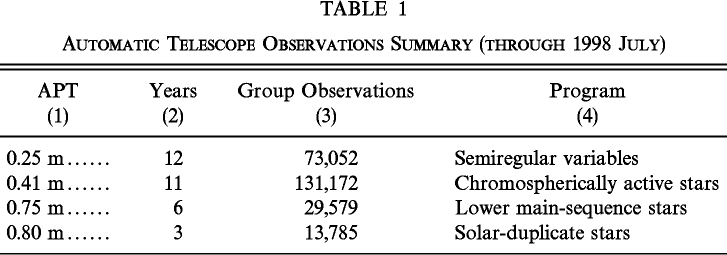
The 0.75 m telescope is identical to the APTs described by Strassmeier et al. (1997), and the 0.80 m telescope is very similar (Fig. 2). The horseshoe equatorial mounts and open‐tube superstructures were designed by Boyd and fabricated by Rettig Machine Shop of Redlands, California. Both APTs have disk‐and‐roller drives on both axes driven by stepper motors through sprocket‐and‐belt reduction systems. The Cassegrain optics were manufactured by Star Instruments of Flagstaff, Arizona. The primary mirrors have f/2 focal ratios; the effective focal ratios are f/8. Boyd, with help from D. Epand (also at Fairborn), produced the control systems that automate the telescopes and photometers. The control systems are briefly described in Strassmeier et al. (1997), and much of their early development is discussed in Trueblood & Genet (1985).
Fig. 2.— The 0.80 m APT at Fairborn Observatory. This telescope, along with a similar 0.75 m APT, is dedicated to a long‐term program of monitoring luminosity cycles in Sun‐like stars. The black box mounted behind the primary mirror is the automated photometer.
Both telescopes are equipped with automated photometers: a single‐channel photometer on the 0.75 m APT and a two‐channel photometer on the 0.80 m. Both were designed and built by Boyd, following the criteria developed in Young et al. (1991). The optical layout of the two‐channel photometer on the 0.80 m APT is shown in Figure 3. All components in the figure, as well as the voltage‐divider chains and the preamplifier/discriminators for both channels, are contained within an insulated and sealed enclosure and cooled to just above the freezing point of water via a liquid coolant bath supplied by an external chiller. In addition, filtered and dried air constantly flows through the photometer to control dust and humidity. Light from the telescope enters through a fused‐silica window in the top of the photometer. Between this entrance window and the focal plane is a filter wheel containing a selection of neutral‐density filters that attenuate the light from bright stars. In the focal plane, a diaphragm wheel provides a selection of diaphragm sizes between 30'' and 90'' as well as a fully open position for target acquisition and a closed position that acts as a dark slide. After passing through the diaphragm, the light beam encounters a flip mirror that directs the light either through a transfer lens to a Pulnix 840N CCD camera (for rapid and accurate centering of target stars in the diaphragm) or toward the detectors. In the detector path, the light first passes through a fused‐silica Fabry lens and is then split into two beams by a dichroic mirror. Strömgren b and y passbands are measured simultaneously by two EMI 9124QB bi‐alkali photomultiplier tubes (PMTs) operated at −1200 V provided by two external high‐voltage power supplies. The Strömgren b and y filters are fixed directly in front of the cathodes of the phototubes. The single‐channel photometer for the 0.75 m APT is very similar except that a single EMI 9124QB phototube measures a star sequentially through Strömgren b and y filters located on an additional filter wheel. Assembly drawings of an identical single‐channel photometer are shown in Figure 2 of Strassmeier et al. (1997).
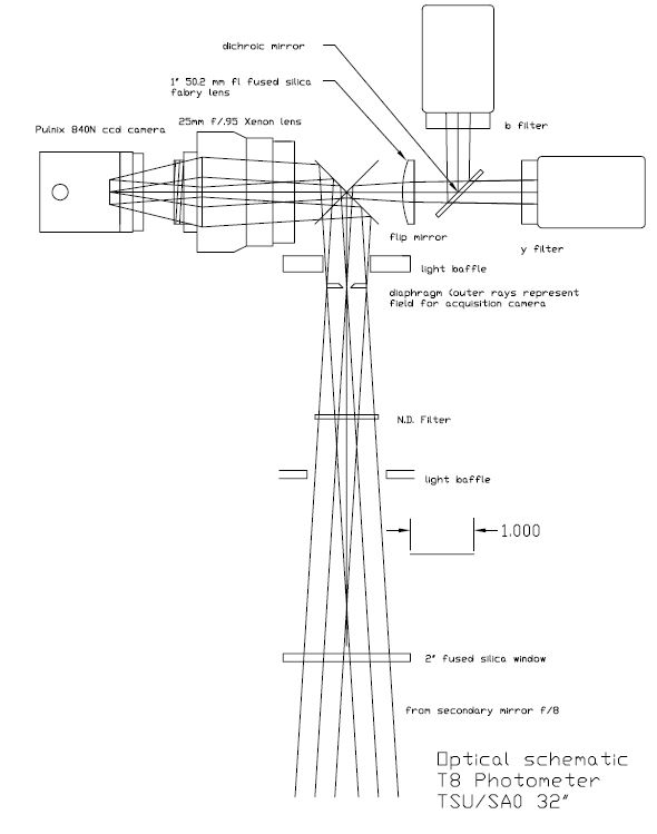
Fig. 3.— Optical layout of the two‐channel photometer on the 0.80 m APT. The CCD camera allows rapid and accurate centering of the star image in the focal‐plane diaphragm, while the dichroic mirror allows two separate PMT detectors to obtain simultaneous observations in the Strömgren b and y passbands.
3. PROGRAM‐STAR OBSERVATIONS
Program stars on the 0.75 and 0.80 m APTs are each observed with three nearby (on the sky) comparison stars in the sequence DARK, A, B, C, D, A, SKYA, B, SKYB, C, SKYC, D, SKYD, A, B, C, D termed a program‐star group, where A, B, and C are the comparison stars and D is the program star. Integration times are 20–30 s (depending on stellar brightness) on the 0.75 m APT, where the Strömgren b and y observations are made sequentially, and 40 s on the 0.80 m APT, where the two bands are measured simultaneously. If a neutral‐density filter is required, the same one is used for all measurements within a group to avoid the necessity of introducing a neutral‐density filter calibration into the data reductions. A 45'' diaphragm is generally used for all integrations unless an optical companion needs to be excluded with a smaller diaphragm. The observations are reduced differentially with the standard equations of Hardie (1962) to form six sets of differential magnitudes: D−A, D−B, D−C, C−A, C−B, and B−A. These differential magnitudes are corrected for dead‐time and differential extinction and transformed to the Strömgren photometric system with coefficients determined from quality‐control observations described in the next section. The program‐star observing sequence results in three measures of each of the six differential combinations in both the b and y colors. The three measures of each combination are averaged to form the group mean differential b and y magnitudes, which are treated as single observations in subsequent analysis.
Each program‐star group requires about 13 minutes of telescope time to complete, so roughly 40 program groups can be completed on an average night by each telescope. The groups are observed once each clear night throughout their observing seasons. Each APT can accommodate roughly 75 program stars on its observing menu, distributed more or less evenly throughout the 24h of right ascension. Observations are generally made only when the air mass is less than 1.5. Therefore, declinations must lie north of about −15° for highest precision.
4. QUALITY‐CONTROL OBSERVATIONS
The combination of stable, dedicated instrumentation and the ability to make extensive quality‐control observations each night on each telescope allows the maximum photometric precision of the APTs to be achieved and maintained over the long term. The quality‐control observations take the form of additional group observations designed for specific purposes.
Dead‐time–group observations provide data for the determination of the systems' dead‐time coefficients. Observations of standard‐star groups are used to derive extinction, transformation, and zero‐point coefficients. Dark counts are made as part of each program‐star observing sequence (see above), and Fabry‐scan groups are run each night for additional diagnostic purposes. These quality‐control observations require only 5%–10% of the telescope time each night and so have relatively little impact on the number of program stars that can be observed. They are described in the following paragraphs.
Each night's quality‐control observations are reviewed the next morning as part of the daily data‐reduction process. Daily review of the data ensures that any problems with the APTs are quickly recognized and corrected. A series of reduction programs scan through the output file from each telescope and display the results at the computer, starting with the dark counts. Monitoring the dark counts is useful for recognizing such things as changes in PMT characteristics, failures in the photometer environmental‐control systems, and other miscellaneous problems (e.g., mice chewing through the coolant or dry‐air supply hoses). Figure 4 shows the dark counts from two nights on the 0.75 m APT. The top panel reveals the normal 2–3 counts s−1 (median) count rate observed when the system is operating properly; variations in the dark counts shown in the bottom panel were traced to inadequate coolant flow caused by a leak in the external cooler.
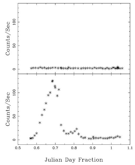
Fig. 4.— Dark counts on two nights from the 0.75 m APT. Count rates of 2–3 counts s−1 (median) seen in the top panel are normal for the photometer temperature of 33°F and operating voltage of −1200 V. Variable dark counts in the bottom panel were due to inadequate coolant flow to the photometer caused by a coolant leak.
The reduction routines next display the result of the night's Fabry scan, one of the most useful tests of the operation of the APTs. The Fabry lens is designed to project a fixed image of the telescope's primary mirror onto the cathode of the photomultiplier tube. Therefore, small deviations in the position of a star in the focal‐plane diaphragm during an integration will not cause significant changes in the measured signal. There are three Fabry‐scan groups on each APT observing menu, spaced at 8h intervals in right ascension. Therefore, one of them can be observed on any night of the year near its meridian crossing. The Fabry‐scan groups command the telescope to center a relatively bright star and then move it just outside the diaphragm. The telescope then steps the star through the center of the diaphragm in right ascension while the photometer takes an integration at each step. The telescope recenters the star and performs a similar scan across the diaphragm in declination. The results from two nights are shown in Figure 5, where the right ascension and declination scans in each case have been offset vertically for clarity. The top scan shows not only that the signal is constant as the star is moved through the diaphragm, but also that the telescope is properly focused and collimated and that the star is being properly centered in the diaphragm by the CCD camera. The broad, asymmetrical wings of the scan in the bottom panel reveal that the telescope is poorly focused and poorly collimated. Currently, there are no autofocus or autocollimation routines on the APTs, so this condition requires manual adjustments. However, errors in focus and collimation can be detected by this technique and corrected before they affect the precision of the photometry.
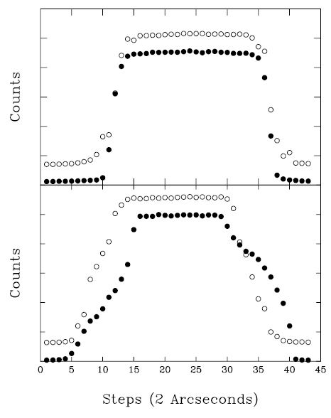
Fig. 5.— Sample Fabry scans from the 0.75 m APT. The top panel shows that the telescope is properly focused and collimated and that stars are being properly centered in the diaphragm. The bottom panel reveals that the APT is poorly focused and collimated.
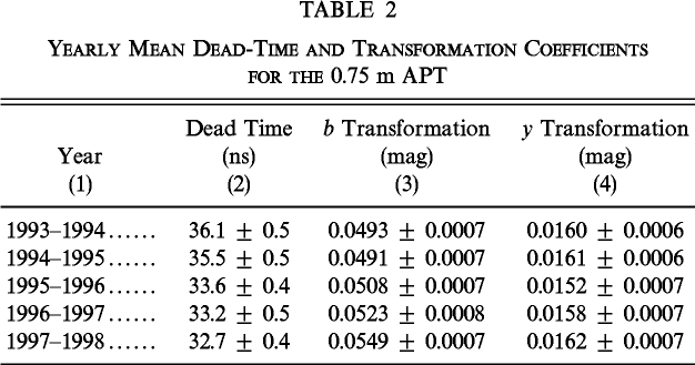
Three dead‐time groups, spaced on the sky at 8h intervals and observed whenever they cross the meridian, permit the nightly determination of the photometers' dead‐time coefficients. These groups consist of two stars, one bright enough to provide a count rate of roughly 500,000 counts s−1 and a second, nearby star a magnitude or so fainter. Integrations on both stars through all of the available neutral‐density filters provide the data needed to derive the dead‐time coefficient and to calibrate the neutral‐density filters (as well as to verify the proper operation of the filter wheels). The daily APT‐reduction routines scan through the output file for all dead‐time groups and add the nightly results to dead‐time coefficient files. Table 2 gives the yearly means of the dead‐time coefficients for the first 5 years of the 0.75 m APT's operation. Because a slow change in those coefficients is observed over time, all observations of standard and program stars are reduced with yearly mean dead‐time coefficients.
 |
As a final step before beginning program‐star reductions, the daily reduction routines search through the output file to find all standard‐star groups to compute the night's extinction, transformation, and zero‐point coefficients. Sixty Strömgren standards from the list of Crawford & Barnes (1970) provide a uniform distribution around the sky and a range in color index. Each standard‐star group consists of a single star, along with a sky position, to be observed in both the b and y colors. Many of the groups are observed at two or three different hour angles to provide a range of air mass. Typically, each telescope acquires 40–50 standard‐star observations each night; they are reduced with least squares to solve simultaneously for nightly first‐order extinction, transformation, and zero‐point coefficients. The reductions automatically reject from the nightly solution standard stars whose residuals exceed 3 σ. The final solution must meet the following criteria: (1) rms less than 0.03 mag, (2) number of stars in the final solution must be 20 or more, (3) air mass must cover the range 1.0 to at least 1.8, and (4) the range in Strömgren (b−y) color index must exceed 0.6 mag. If the solution passes these criteria, the night is considered to be photometric, and the resulting coefficients are saved.
Five years of nightly Strömgren y extinction coefficients from the 0.75 m APT are shown in Figure 6. Gaps in the coverage result because the APTs do not operate during Arizona's summer rainy season; each observing year runs from about mid‐September to early the next July. Seasonal variations are clearly seen in the extinction coefficients. The slight overall decline during the first 3 years (the 1993–1994 through 1995–1996 seasons) resulted from residual effects of the Mount Pinatubo eruption in the Philippines in 1991 June. The slight increase in extinction in the last two seasons (1996–1997 and 1997–1998) was due to the relocation of the APTs from Mount Hopkins (altitude 7600 feet) to Fairborn's new site in the Patagonia mountains (altitude 5700 feet). The program‐star observations on the 0.75 and 0.80 m APTs are reduced with these nightly extinction coefficients.
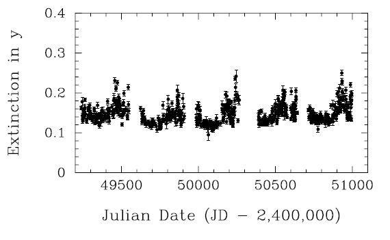
Fig. 6.— Nightly Strömgren y extinction coefficients from the 0.75 m APT. Gaps in the record correspond to the summer rainy season in Arizona when the APTs are shut down. Seasonal variations in extinction are clearly seen; extinction is lowest during the winter months and highest during the spring windy season. Additional subtle effects are described in the text.
Yearly means of the nightly Strömgren b and y transformation coefficients are shown in Table 2. The formal errors in the yearly means are all less than 0.001 mag. The y‐coefficients show no significant change over 5 years; the b‐coefficients show a trend of roughly 0.001 mag per year with the instrumental bandpass getting slightly redder with time. This may be due to aging of the aluminum coatings on the primary and secondary mirrors, which lose reflectivity more rapidly at bluer wavelengths. Nightly observations of the program stars are reduced with these yearly mean transformation coefficients to remove the long‐term trends in instrumental sensitivity. This means that final reduction of the program‐star differential magnitudes and writing to the archives cannot be done until the end of each observing year in July when the mean coefficients for the year can be derived.
While the photometric zero points are not needed in the differential reductions of the program stars, they are, nevertheless, useful for tracking changes in system sensitivity. In particular, they are helpful in deciding when to clean the optics. Figure 7 shows 2 years of Strömgren y zero points from the 0.75 m APT. The zero points decrease slowly over several weeks as dust accumulates on the primary and secondary mirrors as well as on the entrance window of the photometer. When the sensitivity drops 5%–10% (roughly every 3 months), the optics are washed and the zero points recover.
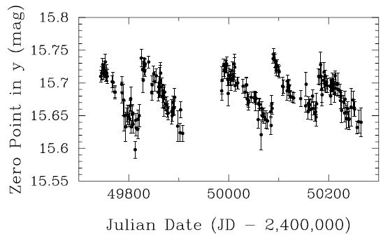
Fig. 7.— Nightly Strömgren y zero points from the 0.75 m APT. The system sensitivity decreases several percent over several weeks as dust accumulates on the optics then recovers when the optics are washed.
5. AUTOMATIC SCHEDULING OF THE OBSERVATIONS
The APTs have no provision for manual operation; there are no eyepieces with which to view the fields or control paddles to slew the telescopes. Observational requests are accepted only via ASCII input files containing such requests in the Automatic Telescope Instruction Set (ATIS) language. These files are communicated to the telescopes from TSU over the Internet. (The last leg of the link to the site is a dedicated phone line to an Internet point of presence in southern Arizona.) In ATIS, a group observation is the primitive unit to be scheduled and executed by the telescope. The various program‐star and quality‐control group sequences executed by the 0.75 and 0.80 m APTs have been described above. ATIS provides a detailed set of commands with which these group sequences can be composed, including commands to move the telescope to a specified target, acquire and center the star in the diaphragm, set the positions of the diaphragm and filter wheels, and make integrations in a specified sequence. Complete details of the ATIS language have been published by Boyd et al. (1993) as part of a special issue on ATIS in the International Amateur‐Professional Photoelectric Photometry Communications. The control systems of the APTs interpret the ATIS commands and generate the hardware‐control signals that carry out the requested observations.
In addition to specifying the syntax and semantics for composing group‐observation requests, ATIS provides a set of group‐selection rules that are used by the telescope‐control software to determine the execution order of groups during the night. These rules operate on parameters specified by the observer and located in the header of each group‐observation request. These parameters include the Julian Date range over which group observations should be made, the hour‐angle limits that are suitable for the group, the number of times the group should be executed within a night, the moon status (up, down, or either) required for the group observation, and a priority. When the telescope is ready to make an observation, the ATIS scheduler first checks all group requests and determines which ones are currently enabled, i.e., which groups are within the limits specified by the group header. From among the enabled groups, any one of which could be executed next, the ATIS scheduler must select the one group that will be executed next. In a simple winnowing process, the scheduler first considers all enabled groups that have the highest priority level. Within that subset of enabled groups, it looks for the ones with the highest observation‐request count. From among those, the scheduler selects the group that is closest to the end of its hour‐angle window, implementing essentially a first‐to‐set‐in‐the‐west policy. In the unlikely event that two or more groups are still tied for next execution, the scheduler simply picks the one that appears first in the ATIS request file. When a group observation has been completed, the scheduler repeats the same process to dispatch the next group for execution and continues doing so for the rest of the night.
This simple ATIS‐dispatch scheduling procedure has been used successfully to schedule all of the Fairborn APTs and has several advantages. First, it is completely robust, i.e., the group selection rules will always converge to the selection of a unique group for execution unless all observation requests have been satisfied. In that case, the telescope simply pauses until additional groups become enabled (for instance, by moving into the beginning of their hour‐angle windows) or the night ends. Second, the scheduler can recover easily from any interruptions due to clouds or equipment failure. Third, a set of groups covering the entire observable sky can be submitted at one time, and the ATIS scheduler will continually schedule the appropriate groups in season for as long as they remain on the observing menu. Fourth, by suitable use of small hour‐angle ranges and higher priorities, the standard‐star and other quality‐control groups can be set up around the sky, and they will be interleaved with the program‐star groups at the appropriate times. The higher priorities of the quality‐control groups ensure the necessary calibration observations are always performed at the optimum times, but since they require only a few percent of the observing time, most of the time is still available for program‐star observations. Finally, good schedules result from the ATIS scheduler if the telescope is properly loaded, that is, when the observing requests contain a suitable density and distribution of groups on the sky. In such cases, the APTs execute program‐star groups beginning at the western limit in the early evening, working toward the meridian by local midnight, ending at the eastern limit at dawn, and interspersing higher‐priority quality‐control groups throughout the night as they become enabled. While simple and robust, the ATIS scheduler is not without its limitations, and improved scheduling methods are under development for the automatic telescopes (see, e.g., Henry 1996; Edgington et al. 1996).
6. PRECISION OF THE PROGRAM‐STAR OBSERVATIONS
Since no human operator is on hand during data acquisition to monitor the photometric quality of the night, the APTs are programmed to collect data as long as they can find stars. Therefore, data taken under nonphotometric conditions must be recognized ex post facto since all program‐star observations are written to the data archives. The first step is to employ a "cloud filter." Neither the comparison stars nor the program stars being observed with the 0.75 and 0.80 m APTs are expected to vary significantly over the several minutes it takes to obtain a program‐star group observation. Therefore, the internal precision of a group observation, measured as the standard deviation of the mean differential magnitude, can be used to filter the data. Figure 8 plots the internal precision of all program‐star group observations from the 0.80 m APT for the 1997–1998 observing season against the air mass of the group observation. Most observations on good nights have internal precisions near 0.001 mag, although this increases slightly at higher air mass. Therefore, when extracting observations from the data archives for analysis, I use a 0.005 mag cloud filter for rejecting observations with uncertainties greater than this approximately 3 σ limit. An entire group observation is rejected by the cloud filter if the internal precision of any of its six differential magnitudes in either color exceeds this limit.
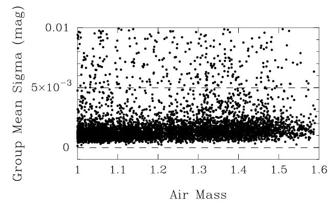
Fig. 8.— Internal precision (measured as the standard deviation of the mean magnitude) of program‐star observations from the 0.80 m APT for all nights of the 1997–1998 observing season plotted against air mass. (Only those with a precision better than 0.01 mag are shown.) Each point corresponds to one complete program‐star group observation. This distribution is used to derive the cloud‐filter level of 0.005 mag, designated by the upper dashed line.
Since the measurement of subtle brightness changes in Sun‐like stars requires data of the highest possible precision, further cleaning of the reduced data, beyond the cloud‐filtering process, is necessary. This is accomplished by selecting only observations that were made on nights with good all‐sky standard‐star solutions. This ensures that the data used in an analysis were taken on good photometric nights and were reduced with well‐determined nightly extinction coefficients. These two filtering steps are done routinely and automatically whenever data are extracted from the archives. This results in the rejection of about half of the observations, since the APTs collect data in both photometric and spectroscopic conditions. These automatic filtering techniques work very well and eliminate most of the poor‐quality data. To identify any remaining outliers, correlation plots of the pairwise differential magnitudes are used to manually reject any remaining discrepant observations before a given data set is analyzed.
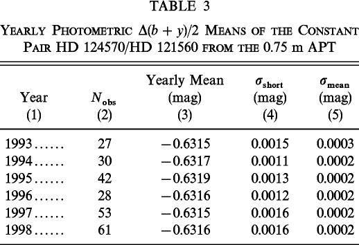
Once program‐star data have been cleaned by this filtering process, their external precision can be determined. External precision is measured on two timescales: short term (night to night) and long term (year to year). Short‐term external precision is measured as the standard deviation of a single group mean observation from the corresponding seasonal mean differential magnitude. This can be easily computed from observations of constant pairs of stars. Table 3 lists results from the 0.75 m APT from differential magnitudes of the constant stars HD 124570 (F6 IV) and HD 121560 (F6 V). Here, the yearly mean Strömgren Δb and Δy magnitudes have been combined into a single Δ(b + y)/2 differential magnitude to increase precision, as done by Lockwood et al. (1997) in their program of Sun‐like star photometry. Column (4) lists the short‐term or nightly precision for each of the six observing seasons. The mean of those six standard deviations is 0.0014 mag, which I take to be the typical external precision of a single observation from the 0.75 m APT. A similar analysis of data from the same pair of stars for the first 3 years of the 0.80 m APT's operation gives 0.0011 mag for its short‐term external precision. This is slightly better than the 0.75 m APT because longer integrations are used with the 0.80 m two‐channel photometer to reduce scintillation noise, which accounts for most of the APT measurement errors.
 |
The observations in Table 3 also allow the determination of the long‐term (year to year) external precision of the 0.75 m APT observations. This is measured as the standard deviation of the yearly mean magnitudes from the mean of the yearly means. The total range of the yearly means in column (3) is only 0.0004 mag; the long‐term external precision is 0.00015 mag. Thus, the observed long‐term precision agrees with the predicted 0.0002 mag uncertainties in the yearly means from column (5), computed as σshort divided by the square root of the number of observations for each year. This 0.0001–0.0002 mag level of precision is also reached by the 0.80 m APT for suitably constant pairs of stars.
7. VARIABILITY IN COMPARISON STARS
Perhaps the greatest impediment to achieving routinely the precision documented above is low‐amplitude, intrinsic variability in the comparison stars, a difficulty also encountered by Lockwood et al. (1997) and Radick et al. (1998). Criteria for the selection of comparison stars for the APTs include (1) closeness on the sky to the program star, (2) color index similar to the program star, (3) brightness (8th mag or brighter to minimize errors arising from photon statistics), (4) membership in a spectral class predominately populated by constant stars, and (5) absence of known variability. The majority of comparison stars were chosen from spectral class F, but a number of cooler stars were used as well, especially G and K giants. However, most of the comparison stars were selected before the release of the Hipparcos Catalogue (Perryman et al. 1997) and, therefore, without the improved parallaxes, magnitudes, color indices, and photometric variability statistics now available from Hipparcos. Many were chosen based only on their HD spectral classifications and proper motions.
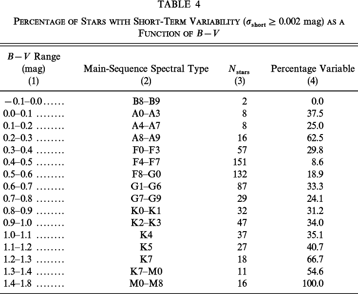
Figure 9 shows observed short‐term photometric variability of comparison and program stars from both APTs in the HR diagram. The Hipparcos magnitudes, color indices, and parallaxes were used to locate the stars on the diagram since nearly every star (714) had an entry in the Hipparcos Catalogue. Main‐sequence stars redder than B−V ∼ 0.5 are the program stars; all others are the comparison stars. Constant stars are plotted as small filled circles. Stars with σshort≥0.002 mag are designated short‐term variables and are plotted with open circles. A few new comparison stars with, as yet, undetermined photometric variability are plotted with crosses. This 0.002 mag level of observable variability is derived from our observations of short‐term variability in Sun‐like stars in Figure 11 (below). In that sample, only stars younger than the Sun have σshort≥0.002 mag, and all stars older than the Sun have σshort<0.002 mag, consistent with expected variability patterns in those stars. Therefore, observed σshort≥0.002 mag in the APT observations implies that photometric variability has, indeed, been detected.
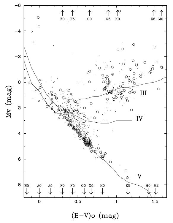
Fig. 9.— Short‐term photometric variability in the HR diagram of 714 comparison and program stars from both the 0.75 and 0.80 m APTs. Main‐sequence stars redder than B−V ∼ 0.5 are the program stars; the rest are comparison stars. Constant stars are plotted with small filled circles; stars with detectable short‐term variability (σshort≥0.002 mag) are plotted as open circles. A few new comparison stars with undetermined photometric variability are plotted with crosses.
It is clear from Figure 9 that low‐amplitude, short‐term variability occurs throughout the HR diagram. Young, lower main‐sequence (late F through K) program stars are variable as a result of their rapid rotation and dynamo‐induced spot activity (e.g., Baliunas et al. 1998; Radick et al. 1998). Many of the comparison stars are F0–F8 dwarfs and subgiants, and short‐term variability occurs in this range as well. At the cooler end of this range, the variability mechanism is probably still spot activity, as variability occurs predominantly in the stars closest to the zero‐age main sequence (i.e., the youngest stars), as is the case for the program stars. Variability occurs in the early‐F (and late‐A) stars both on and above the main sequence. This variability arises from radial and nonradial pulsations in variables like the δ Scuti and γ Doradus stars (e.g., Aerts, Eyer, & Kestens 1998). Most of the G and K giants chosen as comparison stars are also short‐term variables. The variability mechanism in those stars is still unknown (Hatzes & Cochran 1998).
These results on short‐term variability are summarized in Table 4 for various ranges of B−V color index. Corresponding approximate spectral‐type ranges given in the table are for main‐sequence stars. Constant stars are most likely to be found in the B−V range 0.4–0.5, corresponding to spectral types F4–F7, where only 8.6% of stars are variable from night to night. Among stars in the range 0.3–0.4, corresponding to spectral types F0–F3, 29.8% of stars are variable. Stars with B−V later than 0.5 (F8 and later) are either the main‐sequence program stars or the G and K giant comparison stars; both groups exhibit frequent variability. All stars redder than B−V = 1.4 were found to be variable. Stars bluer than B−V = 0.3 are also quite likely to be variable. While the Hipparcos results are useful for locating candidate comparison stars on the HR diagram, it is unfortunate that the Hipparcos photometry lacks the precision to identify a priori which candidate comparison stars are low‐amplitude variables. For instance, in a study of 187 of the G and K giant comparison stars, most of which were variable, Henry et al. (1999b) found that only a few percent of the variables (those with amplitudes of 3%–4% or greater) were identified as such in the Hipparcos Catalogue.
 |
These results seem to indicate that the best comparison stars should be chosen from the spectral range F4–F7. However, when excellent long‐term stability is also required in the comparison stars, the choice is not so clear. Since long‐term (year to year) variability can be measured to a precision of 0.0001–0.0002 mag with the APTs, many stars that are constant to 0.001 mag from night to night are still observed to vary significantly from year to year. Table 5 shows the percentage of stars with measurable long‐term variability (σlong≥0.0005 mag) derived from the 0.75 m comparison and program stars. The 0.80 m APT results are not included since it has not been operating long enough to characterize long‐term variability. In the range F4–F7, where less than 10% of stars are short‐term variables, nearly 60% have detectable long‐term variability. A better place to find long‐term stability is in the range F0–F3; even better odds occur at A8–A9. However, the chance for short‐term variability in these ranges increases from less than 10% at F4–F7 to over 60% at A8–A9. The mid‐F stars presumably have sufficient convection zones that magnetic dynamos still operate within them and drive small, but significant, long‐term brightness changes. The late‐A and early‐F stars lack the magnetic dynamo, but many are pulsating δ Scuti and γ Doradus variables. The disappointing and frustrating result: there seems to be no location in the HR diagram where stars are likely to be found with the desired level of short‐ and long‐term stability.
 |
Since many of the program stars on the 0.75 and 0.80 m APTs are solar age and older, with very small luminosity changes from year to year, the highest possible stability is needed in the comparison stars to resolve unambiguously the variability in the program stars. Consequently, as comparison stars are proven variable, they are replaced with new ones. The replacements are now chosen primarily from among the late‐A and early‐F spectral types, derived from the Hipparcos results, because long‐term stability is so important. While many will turn out to be new short‐term variables, these can be identified in a single season and quickly replaced. Alternatively, if new comparisons are chosen from the F4–F7 stars, several years might pass before it becomes obvious that they are variable. The A8–F3 stars have a very good chance of exhibiting long‐term stability if they lack the short‐term variability. In fact, even the majority of those with observable low‐amplitude, short‐term variability appear to be constant from year to year.
8. OBSERVATIONS OF SUN‐LIKE STARS
The roughly 150 Sun‐like stars being monitored by the 0.75 and 0.80 m APTs are plotted in Figure 10, which shows their distribution in the log R'HK (age) versus B−V (mass) plane. Open circles are from the 0.75 m APT; filled circles are from the 0.80 m APT. The stars range in mass from about 1.3 M⊙ on the left to 0.7M⊙ on the right. They range in age from 100 Myr at the top to 10 Gyr at the bottom. The chromospheric emission ratios (log R'HK) are computed from the Ca ii H and K index as defined and determined by the Mount Wilson HK Project (Baliunas et al. 1998). For comparison, the Sun is plotted as a circled point at a B−V of 0.642 and a log R'HK of −4.901. Most of the 0.80 m APT stars were selected to be close to the Sun in both mass and age. Therefore, this plot does not represent the natural distribution of nearby Sun‐like stars.
Fig. 10.— The distribution in log R'HK (age) and B−V (mass) of the 150 Sun‐like stars being monitored with the 0.75 m APT (open circles) and 0.80 m APT (filled circles). The Sun's position is plotted for comparison.
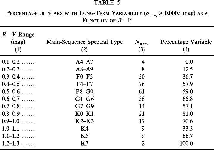
Short‐term photometric variability (σshort) in this sample of stars is shown in Figure 11, where the symbols are used as in the previous figure. The standard deviations are derived from the differential magnitudes computed with respect to a constant comparison star in each case. In this figure, age increases from left to right from 100 Myr to 10 Gyr. As a lower main‐sequence star ages, its rotation slows, its dynamo weakens, and its chromospheric emission ratio decreases. As seen in the figure, this is accompanied by a decrease in the amplitude of short‐term photometric variability. Corresponding standard deviations (σshort) decrease from nearly 0.03 mag to below ∼0.0010 mag, which represents the limit of precision for a single observation. The standard deviations from the 0.80 m APT lie systematically somewhat below those from the 0.75 m APT because longer integration times were used with the two‐channel photometer on the 0.80 m APT. The Sun's day‐to‐day photometric variability is represented by the two circled points, based on satellite radiometer measurements and corrected for the difference between total solar irradiance and the Strömgren b and y bandpasses (Radick et al. 1998). The lower of the two represents the photometric variability of the quiet Sun during sunspot minimum, while the upper symbol represents solar variability during sunspot maximum. It is clear that the APT observations will not, in general, resolve night‐to‐night variations in Sun‐like stars older than the Sun.
Fig. 11.— Short‐term variability (σshort) in the sample of 150 Sun‐like stars observed with the 0.75 m APT (open circles) and the 0.80 m APT (filled circles) as a function of chromospheric emission (age). The Sun's photometric variability during sunspot maximum and minimum is shown by the upper and lower circled points in the inset panel. Night‐to‐night variability less than about 0.0010 mag cannot be resolved.
Figure 12 shows an example of long‐term variability for one of the 0.75 m program‐star groups. There are two program stars and two comparison stars in this particular group. Star D is χ1 Ori (HD 39587), a young (∼800 Myr) G0 V star. Star C is 111 Tau (HD 35296), a young (∼300 Myr) F8 V star. Stars A and B are F0 III and F0 V comparison stars, respectively. The six panels plot the six combinations of differential (b + y)/2 yearly mean magnitudes over 5 years. Error bars are the 1 σ uncertainties computed as the standard deviation of a single observation from its yearly mean divided by the square root of the number of observations for the year. Dotted horizontal lines mark the mean of the yearly means. The total ranges in magnitudes of the yearly means are given in the lower left‐hand corner of each panel; the standard deviations of the yearly means from the mean of the means (σlong) are given in the lower right‐hand corners. Comparison stars A and B exhibit good long‐term stability with σlong = 0.00022 mag for the B−A differentials. The D−A and D−B panels clearly show a long‐term 0.005‐mag variation in χ1 Ori, and the C−A and C−B panels show a similar variation in 111 Tau. The D−C panel shows the relative brightness variation between the two variable program stars. It is clear from these observations that long‐term variations of 0.003–0.005 mag can be followed easily with the APTs.
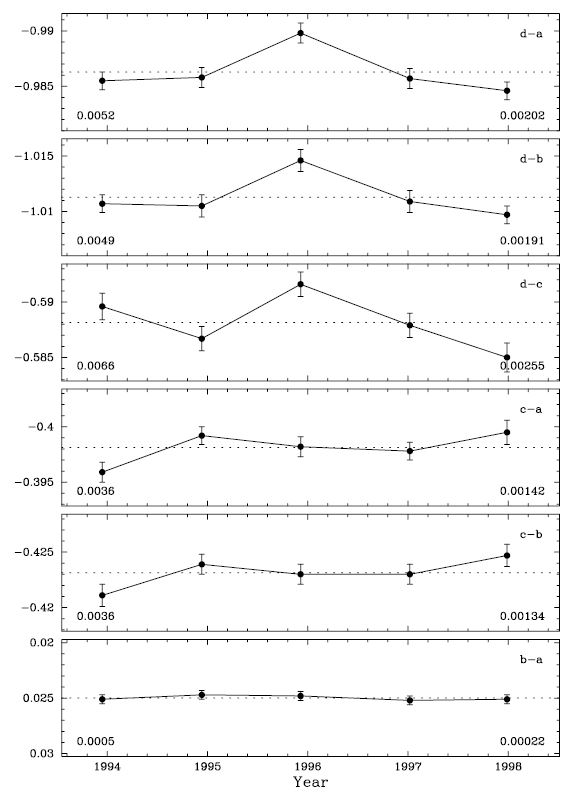
Fig. 12.— Long‐term variability in the young G0 V star χ1 Ori (star D) and the young F8 V star 111 Tau (star C) as observed relative to two constant comparison stars (A and B) with the 0.75 m APT. All six panels have been plotted to the same vertical scale to facilitate intercomparison of the variability observed in the differential magnitudes of each pair of stars. Long‐term variations of 0.003–0.005 mag can be easily traced in these data.
Figure 13 shows the long‐term photometric behavior of the older (∼4 Gyr) G0 V star HD 176051 (star D) relative to three comparison stars HD 173417 (F1 III–IV, star A), HD 178538 (F0, star B), and HD 172742 (F5, star C). Stars A and B show good long‐term stability with σlong = 0.00021 mag for the B−A differential magnitudes. HD 176051 shows clear long‐term variability of about 0.0015 mag in panels D−A and D−B. Comparison star C also shows obvious long‐term variability of about 0.002 mag over 6 years in panels C−A and C−B. Thus, with suitably constant comparison stars, the APTs are also capable of resolving small luminosity changes in the solar‐age program stars.
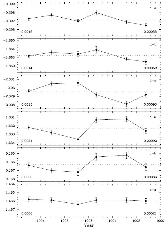
Fig. 13.— Long‐term variability of only 0.001 mag over several years in the solar‐aged G0 V star HD 176051 (star D) is clearly resolved relative to comparison stars A and B with the 0.75 m APT. Comparison star C is also a long‐term variable. All six panels have been plotted to the same vertical scale.
9. SEARCH FOR EXTRASOLAR PLANETS
Recently, several of the Sun‐like stars being monitored by the 0.75 and 0.80 m APTs have been discovered to have planetary‐mass companions with surprisingly short periods (see, e.g., Marcy & Butler 1998 and references within). Since all of the new extrasolar planets have been detected indirectly via radial‐velocity techniques, independent observations are needed to confirm that the observed radial‐velocity variations are not due to star‐spot effects or pulsations in the stars themselves. Since star spots and pulsations should both be accompanied, at some level, by light variations, the APTs can assist in the confirmation of extrasolar planetary candidates by searching for brightness variations in the stars on the reported planetary‐orbital periods (Henry et al. 1997; Baliunas et al. 1997).
Figure 14 shows six seasons of nightly Strömgren (b + y)/2 differential magnitudes of the F7 V star τ Boo from the 0.75 m APT. The observations are plotted modulo the 3.31275 day orbital period of the ≥3.39MJup planetary companion, reported by Butler et al. (1997). Phase 0.0 corresponds to the time of conjunction when the companion would transit the star for suitable orbital inclinations. A least‐squares sine fit at the orbital period yields a semiamplitude of 0.00011 ± 0.00009 mag, indicating no light variability on the planetary period to one part in 104. This supports the hypothesis that the observed radial‐velocity variations in τ Boo are, indeed, due to a planetary companion. The APT photometry also supports similar conclusions for other Sun‐like stars with reported planetary companions (Henry et al. 1997, 1999a; Baliunas et al. 1997).
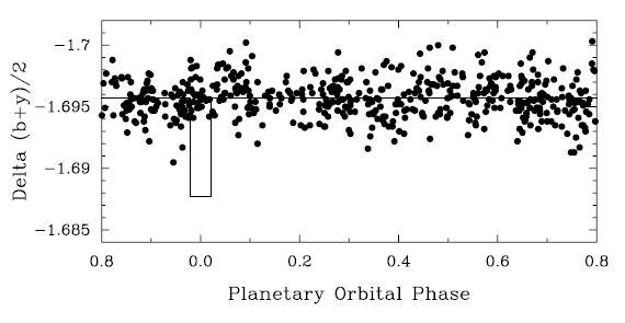
Fig. 14.— Six seasons of nightly Strömgren (b + y)/2 differential magnitudes of the F7 V star τ Boo from the 0.75 m APT plotted modulo the 3.31275 day orbital period of the purported ≥3.39MJup planetary companion. No light variability is observed to one part in 104, supporting the existence of the planetary companion as the cause of the observed radial‐velocity variations in this star.
Figure 15 shows the observations of τ Boo from Figure 14 near the time of conjunction replotted with an expanded scale on the abscissa. An additional night of monitoring observations with the 0.80 m APT has been added. The solid line shows the predicted depth (0.008 mag) and duration (3.6 hr) of the transit for a 1.2RJup planet across the 1.4 R⊙ star. The detection of such a transit would resolve the inclination‐angle ambiguity and allow the actual, as opposed to the minimum, mass of the planet to be computed from the radial‐velocity observations. The observed depth of the transit would provide a measure of the planet's size and, thus, its density. These parameters are important for improving theoretical models of the compositions and origins of these strange, new planets. Figure 15 shows conclusively that transits do not occur in τ Boo. Similar APT observations of six additional Sun‐like stars with Jupiter‐mass planets in short‐period orbits also reveal no transits, in spite of an overall 50% probability of finding at least one transit in the sample. With the discovery of a few additional short‐period planets, the probability for the detection of a transit will increase to around 70%. The successful observation of a transit would represent the first direct detection of an extrasolar planet.
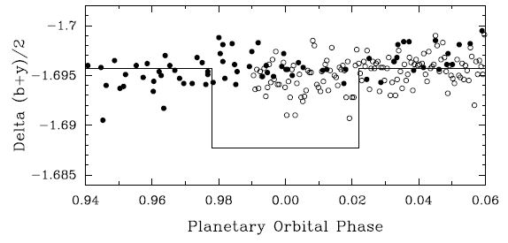
Fig. 15.— Photometric observations of τ Boo from Fig. 14 (filled circles) replotted with an expanded scale on the abscissa. An additional night of monitoring observations with the 0.80 m APT has been added (open circles). The solid line shows the predicted depth and duration for the transits of the planetary companion. Although the probability of transits is 14% in this system, the observations clearly show that they do not occur.
It is a pleasure to acknowledge the work of Lou Boyd and Don Epand at Fairborn Observatory. Without their dedicated efforts over many years, this present work would not be possible. I also acknowledge many helpful discussions with Wes Lockwood about the high‐precision photometry program at Lowell Observatory. I am also grateful to Mike Busby, director of the Center of Excellence in Information Systems, for providing a supportive environment for this work over the past decade. My thanks also go to Stephen Henry for preparing Figure 9 and Tables 4 and 5 from the APT databases. Astronomy with automated telescopes at Tennessee State University has been supported by the National Aeronautics and Space Administration, most recently through NASA grants NAG8‐1014, NCC2‐997, and NCC5‐228 (which funds TSU's Center for Automated Space Science), and the National Science Foundation, most recently through NSF grants HRD‐9550561 and HRD‐9706268 (which funds TSU's Center for Systems Science Research). The planetary search program is also partially supported by the Richard Lounsbery Foundation.
Footnotes
- 1
Further information about Fairborn Observatory can be found on the World Wide Web at http://24.1.225.36/fairborn.html, while the TSU automated astronomy group can be found at http://schwab.tsuniv.edu/.