
ABSTRACT
We have built and used on several occasions an optical broadband stellar polarimeter, PlanetPol, which employs photoelastic modulators and avalanche photodiodes and achieves a photon‐noise–limited sensitivity of at least 1 in 106 in fractional polarization. Observations of a number of polarized standards taken from the literature show that the accuracy of polarization measurements is ∼1%. We have developed a method for accurately measuring the polarization of altitude‐azimuth mounted telescopes by observing bright nearby stars at different parallactic angles, and we find that the on‐axis polarization of the William Herschel Telescope is typically ∼15 × 10−6, measured with an accuracy of a few parts in 107. The nearby stars (distance less than 32 pc) are found to have very low polarizations, typically a few ×10−6, indicating that very little interstellar polarization is produced close to the Sun and that their intrinsic polarization is also low. Although the polarimeter can be used for a wide range of astronomy, the very high sensitivity was set by the goal of detecting the polarization signature of unresolved extrasolar planets.
Export citation and abstract BibTeX RIS
1. INTRODUCTION
Polarimetry is a technique that is capable of achieving very high sensitivity, even with ground‐based telescopes. It is a differential technique that in principle is not affected by the Earth's atmosphere and is limited only by photon noise. Despite this, most polarimeters used by nighttime astronomers achieve fractional polarizations of only 10−4. They mostly employ slow modulation using wave plates in step‐and‐stare mode and use simultaneous dual‐beam measurement of the orthogonal polarization states to remove the effects of the atmosphere on aperture polarimetry of point sources. However, in such systems the sensitivity is limited by the precision to which the two beams are calibrated. By contrast, systems with fast modulators remove the need for high precision by separating the polarized flux from the unpolarized flux and measuring the former as a signal in the time domain. In principle, this does not require a dual‐beam system. Additional drawbacks of using modulators with mechanical rotation are that image motion on the detector, arising from any nonparallelism in the wave plate, will introduce errors from incomplete flat‐fielding, and dust on the wave plate can cause additional modulation of the light intensity.
Solar astronomers, who generally use fast modulators such as photoelastic modulators (PEMs) or ferroelectric liquid crystals (FLCs), have achieved sensitivities of ∼5 × 10⁻⁶ (Stenflo 2003), and Kemp et al. (1987) measured the integrated light from the Sun, giving an upper limit for the fractional linear polarization of 2 × 10⁻⁷. Kemp et al. used a PEM polarimeter that directly viewed the Sun, rather than using an intermediate telescope, and hence avoided the potential problem of telescope polarization.
The main scientific driver in building a polarimeter with very high sensitivity was the detection of the polarization signal from the so‐called hot‐Jupiter extrasolar planets, and hence a direct detection of the scattered light from the planet (for a recent review of extrasolar planets, see Marcy et al. [2005]). There are significant advantages in direct detections of the light from such planets, which at optical and near‐infrared wavelengths will be light from the central star reflected off the planetary atmosphere. Such direct detections, particularly with color information, can provide information about the planet's albedo and radius and the nature of the scatterers in the planetary atmosphere. To date, extrasolar planets have been detected mostly by indirect means, principally through radial velocity measurements of the central star or, far less frequently, through reductions in brightness of the star as a planet transits. Recently, Deming et al. (2005) and Charbonneau et al. (2005), using Spitzer observations, reported the detection of mid‐infrared radiation from HD 209458b and TrES‐1b, respectively, by observing the reduction in flux during secondary eclipse, when the planet passes behind the star. To date, there are no detections of the reflected light from planets, and for the hot Jupiters with orbital radii less than 0.1 AU, there is little prospect of being able to spatially resolve them from the very much brighter central star in the foreseeable future. Hence, to study their atmospheres, very high sensitivity observations have to be made in order to separate the reflected light from the direct stellar light.
For the simple case of a Lambert sphere, Seager et al. (2000) showed that the maximum reflected light from a planet, relative to the direct light from the star and occurring at full phase, is given by  o = 2/3(Rp/D)2, where Rp is the planet radius and D is the planet‐star distance. For a hot Jupiter, typically Rp = 1.5 RJ (Rp for HD 209458 is 1.54RJ ± 0.18RJ, from transit observations [Mazeh et al. 2000], where RJ is the radius of Jupiter) and D = 0.05 AU, making o∼1.5 × 10⁻⁴, with a maximum orbital change of ∼150 μmag for an inclination i of 90°. Currently, such very small changes in the brightness of the star‐planet system are too small for ground‐based telescopes to observe. Assuming Rayleigh scattering, the observed fractional polarization will range from zero for orbital phase angles of 0° and 180° to a maximum of ∼5.5 × 10⁻⁵ at ∼70° and ∼290° for a hot Jupiter (i = 90°). Using more detailed models, Seager et al. (2000) give peak fractional polarizations that are typically a few ×10−6, but with significant variations in the peak polarization and orbital signature, depending on the assumptions made on the nature and size of the atmospheric particles. Thus, measurement of the polarization of these systems is likely to require polarization sensitivities of ∼10−6.
The rest of the paper is structured as follows. In § 2 we outline the instrument design and review the data reduction procedure. Section 3 models the passband, and § 4 describes the method of determining the telescope and instrument polarization and the calibration and performance of the polarimeter. Sections 5 and 6 discuss the effect of atmospheric conditions and the science programs, respectively, and then finally, § 7 presents the conclusions and future developments.
2. INSTRUMENT DESIGN
The polarimeter, known as PlanetPol, was designed for use on a range of telescopes, mounted at the unfolded Cassegrain so as to minimize telescope polarization. As with any polarimeter, it is important that the first optical element, apart from calibration polarizers, is the modulator, immediately followed by the analyzer. However, as a two‐beam analyzer is used, it was found necessary to include the aperture stop, which is at the main telescope focus, between the modulator and analyzer (see Fig. 1). Following the analyzer are wheels with color and neutral density (ND) filters. An electromechanical shutter (not shown) is located between the aperture wheel and the Wollaston prism. Fabry lenses image the primary mirror onto single‐element detectors, sufficient for a stellar polarimeter, and also eliminate any problems with flat‐fielding. PlanetPol has two channels: the star channel on the telescope axis giving the minimum telescope polarization, and a sky channel offset by 95 mm (428'' at the William Herschel Telescope [WHT]). Sanchez‐Almeida & Pillet (1992) give the telescope polarization as being proportional to the square of the distance from the telescope axis, which is ∼10−4 for a 1° offset at 650 nm. With PlanetPol mounted on the WHT, this translates to a telescope polarization of ∼1.5 × 10⁻⁶ for the sky channel, although this assumes a telescope with perfect optics; normally, higher values would be expected. In practice, any increased telescope polarization in the sky channel is not a problem, since the sky signals are much lower and hence the polarized flux contribution is very low. Brief descriptions of PlanetPol are given in Hough et al. (2005, 2006).
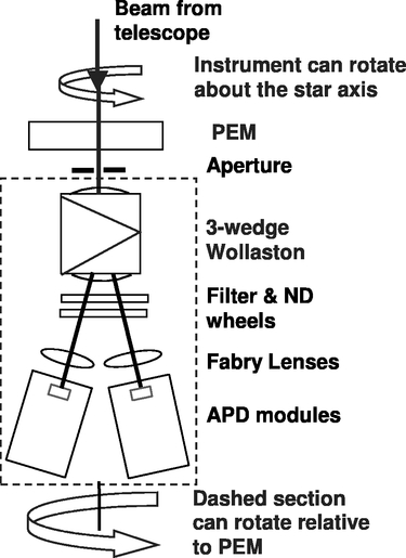
Fig. 1.— Schematic of PlanetPol. There are two identical channels, with only one shown here: the object channel is on the telescope axis, and the sky channel is offset by 95 mm. The instrument is rotated through 45° to measure the second linear Stokes parameter. The Wollaston analyzer, together with the filter and detector assemblies, is rotated by 90° (from −45° to +45°) relative to the PEM axis, changing the polarity of the modulated signal and thereby minimizing systematic errors.
2.1. Modulator and Analyzer
The highest sensitivity polarization measurements, such as those pioneered by J. C. Kemp (Kemp et al. 1986 and references therein), have made use of PEMs, in which a slab of nonbirefringent material is stressed using piezoelectric actuators at the natural frequency of the slab, f0, so as to reduce the power needed to sustain a standing wave in the slab. Such devices are ideal as polarization modulators, as they operate at frequencies of tens of kHz, well above seeing or scintillation fluctuations produced by turbulence in the Earth's atmosphere. Furthermore, they do not involve any rotating parts and so do not produce any periodic motion of the image on the detector, nor any periodic fluctuations in signal caused by dust on the modulator, both of which might lead to spurious polarization signals. Another distinct advantage of PEMs is that they can be used in fast beams, thus eliminating the need for any prior optics that could change the polarization state of the incident radiation. Kemp (1969) shows that the change in retardance Δφ is given by Δφ/φ∼0.5 × θ2, where φ is the retardance and θ is the angle of incidence. For the f/11 beam of the WHT, this translates to a spread in retardance of ∼0.1%, which is negligible compared to the spread in retardance that arises from the use of broad color filters. It is possible that changes in the physical focus of any telescope, arising from changes in the temperature of the telescope, will lead to a change in the f‐ratio of the beam passing through the PEM. All observations reported here were made at the WHT, where dynamic control maintains the position of the focal plane to better than 0.03 mm. Even a 10 mm change in focus leads to a change of only 0 002 in the angle to the normal of the extreme rays hitting the PEM, giving a change in retardance that is less than 1 part in 106.
For PlanetPol, a limit was set on the maximum frequency of the PEM by the 70 kHz bandwidth of the detectors (see § 2.2). As the linear polarization signal is detected at 2f0, a PEM with f0 of 20 kHz was chosen (note that second‐harmonic detection eliminates dichroic surface transmittance, an oscillating linear polarization produced at the surface of the modulating device; Kemp et al. 1987). This is at the bottom end of the frequency range of PEMs, and hence the physical size is relatively large. Specifically, PlanetPol uses an I/FS20 fused‐silica PEM from Hinds Instruments, with a PEM90 controller. It can be used between λ = 170 nm and 1 μm and was supplied with a broadband AR (antireflection) coating optimized for the PlanetPol wavelength range of 470–910 nm, centered at 690 nm. The large size of the I/FS20 leads to the relatively large useful aperture of 22 mm, which Hinds defines as giving ≥90% of the maximum retardance (the average efficiency is ∼99% within 22 mm). For an f/10 beam, the fastest used by PlanetPol, the beam width at the PEM is ∼6 mm, well within the useful aperture.
PlanetPol uses a three‐wedge calcite Wollaston prism manufactured by B. Halle, with an extinction ratio of ∼10−6. A three‐wedge Wollaston has far better image quality for a given beam divergence than the two‐wedge version. The prism wedge angle is 216, giving a divergence of the extraordinary rays (e‐rays) and ordinary rays (o‐rays) of 20° at a wavelength of 600 nm. The o‐ and e‐rays for a three‐wedge Wollaston prism make slightly different angles with respect to the incident beam, of an order of 025, but this is not important, as the detectors are individually aligned for each beam. In addition, the reflection losses for the two beams are not equal, and therefore the two beams do not have the same intensity, even for an unpolarized incident beam. Again, this is not an important effect in PlanetPol. As the modulation frequency of the PEM is higher than the frequency of atmospheric fluctuations, there is in principle no requirement to use a two‐beam analyzer with simultaneous measurements of the e‐ and o‐beam intensities to obtain high‐accuracy polarimetry. The two‐beam polarimeter does provide double the throughput, which is very important in measuring very small fractional polarizations. The Wollaston prism has an AR‐coated, cemented plano‐convex lens on the entrance face, which produces a collimated beam. There is also an AR‐coated plano‐convex lens cemented to the exit aperture of the Wollaston, which produces a narrower beam for the Fabry lenses, making their design easier.
When using a single PEM, only one Stokes parameter can be measured for linear polarization; the second Stokes parameter is measured by rotating the instrument through 45°. It is possible to rotate PlanetPol to angles of +90° and −45°, enabling any polarization produced by the instrument itself to be determined. So as to minimize systematic errors, the analyzer, together with the filter and detector assemblies, is rotated by 90° (from −45° to +45° relative to the PEM axis), changing the polarity of the modulated signals (the advantages of this "secondary chopping" are described by Kemp & Barbour [1981]). All rotations are measured using absolute encoders, with a precision of 00055.
2.2. Detectors
The very high modulation rates of PEMs are incompatible with the readout rates for CCDs, although the ZIMPOL polarimeters (Stenflo 2003) use the charge‐shifting and storage capabilities of CCDs to act as a synchronous demodulator, thus overcoming the readout limitations. PlanetPol is designed as a stellar photopolarimeter; hence, spatial information is not required, and the use of single‐element detectors provides both simplicity and low cost. Avalanche photodiodes (APDs) produce more noise than the dynode chain in photomultiplier tubes; however, they do have higher quantum efficiency than photocathodes, they are able to handle very high photon fluxes, and as they have less noise than the external amplifier of a photodiode, they are the best detectors for the photon rates expected with PlanetPol. The APDs used in PlanetPol are Hamamatsu C4777‐SPL‐S2383‐70K's employing a two‐stage thermoelectric cooler and operating with a gain of M = 100, a spectral response covering 400–1000 nm, and a frequency response of 0–70 kHz (3 dB). The active area of the detector has a nominal diameter of 1.0 mm, with the area of uniform response having a diameter of ∼700 μm. The noise‐equivalent power is ∼2 fW Hz−1/2, with a gain of 5.0 × 10⁸ V W−1, a minimum detection limit of 0.53 pW rms, and a maximum input light intensity of 26 nW (giving an output voltage of ∼13 V), with a damage threshold of ∼1 mW input power.
The Fabry lenses, which are mounted on the front of the APD modules, provide a 700 μm diameter beam, matching that part of the APD that has the most uniform response. An excellent "top‐hat" response is obtained as a star image is tracked across the aperture (5 2 at the WHT), and although there are some differences in the responsivities of the detectors, these are constant and can be accounted for in the calibration of polarization degree (see § 4.3).
2.3. Signal Processing and Instrument Control
Each signal channel uses a Stanford Research Systems SR830 DSP lock‐in amplifier to extract the signal modulated at 40 kHz (twice the stress frequency of the PEM), with this 2f (second harmonic) reference frequency for the lock‐in amplifiers supplied by the PEM control units. They are connected to an Arcom industrial PC via a standard GPIB interface that controls the lock‐in and reads the data. The DC signal from the detectors is fed to a 16 bit analog‐to‐digital converter (ADC) housed in the PC. Because the modulated signal, which is proportional to the polarized component of the light, and the DC signal, which is proportional to the light intensity, are measured using different signal processing, care has to be taken in the relative calibrations (see § 4.3). However, it is easier to produce a high‐sensitivity polarimeter using this technique, as the more usual dual‐beam polarimeters, employing a wave plate in step‐and‐stare mode with an area detector, cannot measure fractional polarizations of 10−6 unless the sensitivities of the two beams are calibrated with 10−6 precision.
The PC is also used to control all the mechanical functions of PlanetPol, with the control and data acquisition software implemented using Agilent VEE Pro 6. Communication with the PC is made via an AdderLink KVM Extender, using a dedicated Ethernet line to a remote monitor and keyboard in the observatory control room.
2.4. Filters
These are mounted in two wheels, with six positions for each wheel. The B, V, R, and I color filters, AR‐coated on both surfaces, are from the Bessel photometric filter sets supplied by Omega Optical. Two additional filters, OG590 and RG695, are also included in the filter wheel, allowing the use of very wide passbands (see § 3). The ND filters are from Omega Optical.
2.5. Observing Sequence and Data Reduction
A typical observing sequence for one linear Stokes parameter consists of four or eight runs, each of 30–180 s duration, with the analyzer set alternately to −45° and +45° relative to the PEM. The number and length of each sequence is chosen depending on the brightness of the source. The secondary chopping (see § 2.1), reversing the sign of the modulated signal, is needed to calculate the "polarization offsets" described below. The instrument is rotated through 45° in order to measure the second Stokes parameter. Figure 2 shows a typical real‐time display of the outputs from the lock‐in amplifiers for the star channel with three different fractional polarizations. Note that the signal for a fractional polarization (Q/I or U/I) as low as ∼13 × 10−6 can be clearly seen when the secondary chopping reverses the sign of the signals.
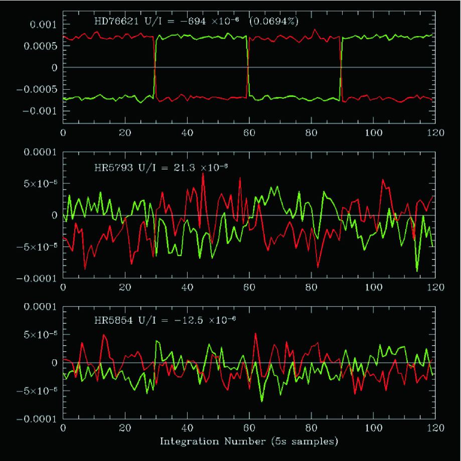
Fig. 2.— A composite of the real‐time displays of the outputs from the lock‐in amplifiers for fractional polarizations of ∼700 × 10−6, ∼20 × 10−6, and ∼13 × 10−6. The two colors represent the outputs from the Wollaston prism with the phases switched when the Wollastons are rotated by 90°. The fractional polarizations shown are not calibrated.
The data acquisition software writes the detected modulated signal values from the four lock‐in amplifiers to four separate files. The DC values, representing the total flux detected by all four detectors, are all output to a fifth file. All five files contain time stamp information at intervals of approximately 20 s. An IDL script that is run on a laptop sharing files with the PC then calculates the measured polarization (Q/I or U/I) of the target star from these data, in the following manner (see Fig. 3 for example displays produced by the IDL script):
- 1.Data from all five files are read into two‐dimensional arrays, each consisting of n steps and k elements. The n steps each represent a block of data that are compiled while the instrument configuration is constant. The k elements within each step each represent a single datum. Typically, the DC signals and the output signals from the lock‐in amplifiers are sampled at 2 Hz, so a step of 180 s contains up to 360 elements. Some data from the beginning of each data stream are thrown away at this point in order to ensure that the four DC signals and the four modulated signals are contemporaneous to within 0.5 s.
- 2.Efficiency factors very close to unity are applied to all the data streams to correct for any slight differences in the responsivity of the four APD detector modules, as measured in the laboratory, and the electronic gains of the lock‐ins and ADCs in each of the four signal trains, which are measured for each observing run prior to mounting the instrument on the telescope. In addition, optical efficiency factors are applied to the two sky channels so that each modulated signal has the same throughput as the corresponding star channel. This ensures that the modulated flux measurements in the sky channels can be used to accurately subtract the flux from the sky in the star channels (see item 5 below). The overall polarization efficiency, and hence calibration of the absolute degree of polarization, is described in § 4.3.
- 3.The smallest value of k out of all five files and all n steps is determined, and the data are placed into new, truncated arrays with equal sizes for all four modulated signals and the DC signals. The lengths of the signal streams differ very slightly in the original files, since they are written sequentially.
- 4.Any "polarization offsets" are calculated for the two star channels. These are small offsets from zero (a few ×10−6) of the modulated signal, proportional to the DC flux of the target star, whose origin is unclear. They are not truly polarized signals, however, since they do not change sign after second‐stage chopping. The offsets differ for each star channel, so they are calculated by summing all data from each channel without making the usual sign corrections for second‐stage chopping. Variance weighting that is proportional to the DC flux level is used in the calculation in order to maximize the precision of the calculation in cloudy weather conditions. The measured offsets appear to be stable over the course of a 1 week observing run. The offsets are the reference levels relative to which polarized flux signals from a star are measured, so any variation in the offsets during an observation would increase the measured standard deviation of a polarization measurement and could lead to an erroneous result. However, the standard deviations for measurements of each low‐polarization standard are extremely stable, indicating that any variation in the offsets is too small to have a measurable effect.
- 5.The polarization (Q/I or U/I) for each star channel is then calculated in a similar way using the variance‐weighted average of the calculation for the full data stream: P1 = ± [(star1 - sky1)/(DC1 - DK1) - offset1], where star1 is the modulated signal in the first star channel, sky1 is the modulated signal in the first sky channel, DC1 is the DC signal in the first star channel, and DK1 is the DC signal level with the shutter closed (which is small and constant for each detector at each gain setting). Offset1 is the "polarization offset" for the first star channel. The plus sign is used for odd steps in the observing sequence, and the minus sign is used for even steps, for the purpose of removing the reversals in sign caused by second‐stage chopping of the analyzer and detector assemblies. This plus/minus sign also removes the effect of the polarization offsets on the results of the time‐averaged calculation.
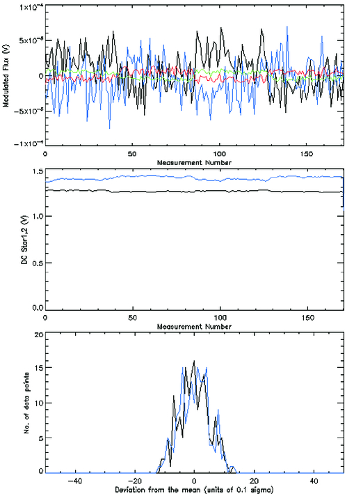
Fig. 3.— Example displays produced by the IDL script from a single Stokes U observation of a nearby star (HR 6148), illustrating the detection of a fractional polarization of 16.5 × 10⁻⁶ due to the sum of TP, IP, and the interstellar medium. The measured polarized flux is visible in the voltage signals in the top panel, which trace the rms amplitude of the 40 kHz sinusoidal modulation with second‐stage chopping. Note the "polarization offsets" (see item 4) with the star channel outputs (black and blue lines) offset from zero. The fractional polarization is the ratio of the modulated signals to the DC signals shown in the middle panel. The modulated flux from the sky channels (green and red traces) has been multiplied by 10 here but still appears weaker, and the sky DC flux is too low to measure. The bottom panel displays the distribution of fractional polarization values about the mean for the two star channels. This appears approximately Gaussian, with no outlying points.
Note that polarization offsets in the sky channels are insignificant, since the sky DC level is usually too low to be measured. The sky channels exist so that modulated flux from the sky can be measured and removed. We find that modulated sky signals make a significant contribution only in very bright conditions (moonlit cirrus clouds or twilight) when using a 5'' aperture. The value of polarization (Q/I or U/I) as a function of time is also stored in an array for each channel (P1, P2) using the unweighted results of the above equation.
The final value of the polarization (Q/I or U/I) is then calculated by averaging the results of the two star channels (after correcting for the difference in sign) and dividing by 0.687, which is the theoretical polarization efficiency of a PEM operating at half‐wave retardance amplitude (see below), when the recorded measurements are the rms value of the detected 40 kHz sinusoidal modulation. This average represents a Stokes Q/I or U/I measurement, depending on the orientation of the instrument. The standard deviation of all data points is then calculated. This determines the random error on a measurement, with a precision of typically 5%–10%, depending on the sample size. This does not include the systematic errors in polarization caused by the telescope and the instrument, which are described in § 4. Finally, the data streams and polarization (Q/I or U/I) values as a function of time are displayed graphically, usually binned for clarity. A histogram of the deviation from the mean of all the individual polarization (Q/I or U/I) measurements in P1 and P2 is also plotted to aid in the detection of any noise spikes, which are extremely rare (see Fig. 3).
Note that for objects with significant polarization (>1%), the efficiency factor of 0.687 is not strictly correct, although in practice the factor 0.687 can be used for polarizations below 10%. For completeness, the full equation, e.g., for Stokes Q, is P1 = ± [0.687(Q/I)]/[1∓0.3042(Q/I)], where the choice of sign depends on the angle between the fast axis of the PEM and the polarization plane transmitted by the Wollaston prism for a particular channel. During each step, this angle will be +45° for one channel and −45° for the other, but the angles will swap several times during an observing sequence. Hence, the denominator effectively remains very close to unity, except in conditions of time‐varying throughput (e.g., cloudy conditions) or when Q/I or U/I is of order unity. When using the simple 0.687 factor in such conditions, the average of the two channels will still be very close to the correct result, although results from the individual channels will be different. The derivation of the full equation is given in
3. THE PASSBAND MODEL
Most observations with PlanetPol have been made with a very broadband red filter covering the wavelength range from 590 nm to the detector cutoff at about 1000 nm. With such a wide band, the exact effective passband and effective wavelength will depend on the color of the object being observed. The polarization efficiency will also vary across the band, as the PEM only gives half‐wave retardance at one wavelength.
To account for such effects, we have developed a detailed model for the passband response, which operates as follows. We start with a spectral energy distribution (SED) appropriate to the source being observed. For this purpose, we typically use one of the Kurucz (1993) stellar atmosphere models. This SED can optionally be modified by applying an interstellar extinction correction using the empirical model of Cardelli et al. (1989). The SED is then corrected for its passage through the Earth's atmosphere by multiplying by an atmospheric transmission spectrum derived from a radiative transfer model for the Earth's atmosphere. This model uses a line‐by‐line treatment of the molecular absorption, using line data from the HITRAN database (Rothman et al. 2005), together with Rayleigh scattering. The Earth atmosphere spectrum is calculated at a resolution that fully resolves the molecular absorption lines. This means that it can be straightforwardly adjusted for any air mass, something that is no longer possible when it is binned to a lower resolution.
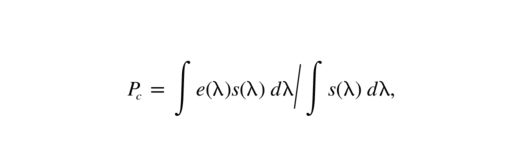
Finally, this spectrum is multiplied by the instrumental response function determined by the filter transmission and the detector responsivity (in A W−1) to give the wavelength distribution of the detected signal (i.e., the relative contribution to the detector current as a function of wavelength). If this spectral distribution is s(λ), then the effective wavelength of the filter is given by
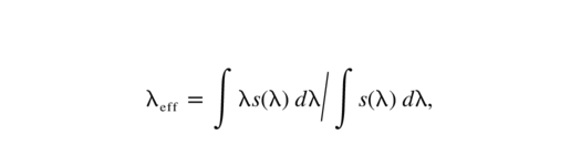
where the integral is taken over all wavelengths at which the instrument has any response. The polarization efficiency correction due to the variation of retardance of the PEM over the bandpass is given by
where

is the wavelength dependence of the efficiency of a PEM polarimeter with the retardance set to half‐wave at wavelength λc, and J2(x) is the Bessel function of order 2. Note that this gives a steeper falloff in efficiency than the sin [π/2(λc/λ)] factor used with retarders, such as wave plates.
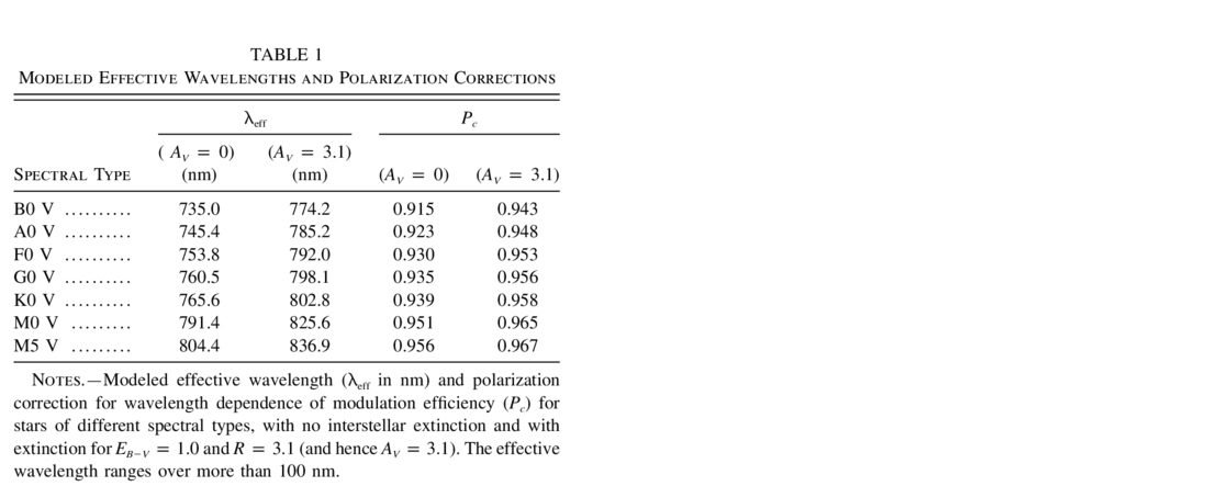
Values of λeff and Pc for a range of stellar spectral types and extinctions are listed in Table 1. The effects of changing the air mass and the water vapor content used in the atmospheric model have also been investigated but are found to be negligible for practical purposes. Changing air mass from 1 to 2 typically shifts the effective wavelength by less than a nanometer and does not change the polarization efficiency. An example of the response curve model is shown in Figure 4.

Fig. 4.— Components making up the passband response model.
 |
4. PERFORMANCE
The following sections describe the performance of PlanetPol, including the measurement of telescope polarization, instrument polarization, and polarized standards from the literature, recorded at the WHT during three runs covering the period 2004 April to 2005 April. These runs represent a total of 21 nights' allocated time, with science data being taken on 12 of them. All observations have been made with a 52 aperture, and the WHT autoguider was used for all observations.
4.1. Telescope Polarization
When measuring fractional polarizations of ∼10−6, it is necessary to determine the telescope polarization (TP) so that the absolute error in TP is significantly less than 10−6. It is much easier to do this if the polarimeter is mounted at the unfolded Cassegrain, where telescope polarization is expected to be at a minimum, typically 10−4 or less.
The TP was determined by observing bright nearby stars (typically within 25 pc) with the telescope derotator enabled, causing the TP to rotate while the interstellar polarization and instrument polarization are fixed. Measuring the polarization of these nearby stars as a function of parallactic angle should, in the absence of any intrinsic stellar or interstellar polarization, produce a sinusoidal curve in Q/I and U/I, with an amplitude equal to the TP, phase‐shifted by 45°. The observations are timed to well sample the range of telescope parallactic angles so that the Cassegrain‐mounted instrument maximally rotates relative to the telescope optics responsible for the TP.
The reduction procedure described in § 2.5 provides measurements of Stokes Q/I or U/I data points for individual observations, typically a 12 or 24 minute integration. Hence, the TP is split into Stokes Q/I and U/I components in changing proportions that can be fitted and subtracted.
The model for the observed signal from each bright star is then
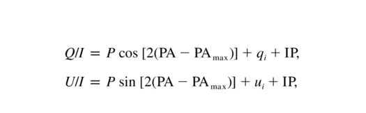
where qi and ui are respectively the astronomical Stokes Q/I and U/I signals from star i, which are assumed to be constant, P is the amplitude of TP, PAmax is the parallactic angle or position angle corresponding to maximum TP in Stokes Q, and PA is the parallactic angle of the observations. The term IP is the instrumental polarization, which is a constant in the model (see § 4.2).
These equations are solved simultaneously for P, PAmax, and the qi and ui values for all the nearby bright stars. Note that only stars with qi and ui<15 × 10-6, and no close binary companion, are used. The equations are solved using a FORTRAN program that makes a least‐squares fit to the deviation of the data from the model, following a Gauss‐Newton minimization approach, to efficiently search the parameter space in an iterative manner (see
The standard errors on P and PAmax that were derived from these Monte Carlo tests agree well with those derived by comparing the results of fits to independent subsets of the real data. However, the reduced χ2 parameter for the fits to all of the full data sets is always in the range of 2.6–3.6, indicating that the individual measurements depart from the fit by more than the expected amount, which was determined by adding the random errors and the uncertainty in TP in quadrature. This is borne out by a larger than expected scatter in the qi and ui values derived for individual stars by fitting subsets of the data. Further investigation showed that the ratio R of the standard error on qi and ui (calculated from the residuals to the fit of the full data sets) to the expected uncertainties has an average value of R = 1.6–1.8 for all stars in each run, consistent with the χ2 parameters quoted above. The value of R varies widely for individual stars, since the number of measurements is generally small, but there is no sign that a floor exists in the achievable precision for very bright stars or stars observed a large number of times. (This appears to be borne out by preliminary analysis of a fourth data set obtained in 2006 February, which included one star with Imag = 0.2 and another that was observed many times. Small values of R are found for both.) Note that since IP is independent of parallactic angle, it does not contribute to the expected residuals to the fit.
Figure 5 (left) shows the directly measured Qinst‐polarization as a function of parallactic angle for a number of nearby stars (where Qinst is not in the equatorial coordinate system). The curve is the same as that shown on the right, in which a Gauss‐Newton minimization has been used, allowing each star to have an interstellar and/or intrinsic polarization. Figure 6 shows both the directly measured Qinst polarization (left) and Uinst‐polarization (right) for stars with a very small interstellar/intrinsic polarization, showing the expected 45° phase shift between the Q‐ and U‐polarizations. A typical fit gives a TP amplitude of (16.4 ± 0.4) × 10-6.
In principle, the procedure would be most accurate if only one or two nearby stars were used, in order to minimize the number of free parameters. However, in the first few PlanetPol runs, we have used four or five stars in order to (1) allow redundancy in case some did not have constant polarization, and (2) provide a range of spectral types (A0 to M0) to determine whether TP changes due to the slight change in effective bandpass. Tests of the fitting procedure with different combinations of stars indicate that TP is independent of spectral type (to within measurement error). In addition, most stars (even young debris disk systems) appear to have constant polarization over at least the timescale of an observing run. The constant polarization of most stars can be attributed to extinction by aligned interstellar dust grains.
The TP itself appears to be constant over the timescale of an observing run. It was found that TP rose from 16 × 10−6 to 18 × 10−6 (with a small change in PAmax) over the 6 month interval between our first two runs. It then dropped to 10 × 10−6 by the third run 6 months later (with a large change in PAmax), this occurring shortly after the telescope's primary mirror had been realuminized. TP is therefore believed to be caused by nonuniformities in the reflecting surface of the primary mirror. It remains possible that the secondary mirror support spider and the secondary mirror surface make a small contribution.
A small TP is also important in minimizing the effects of any nonlinearities in the detection system. Following Keller (2002), if the measured signal S is a quadratic function of the intensity (S = aI2 + bI + c) and δI is the TP signal, then for the case of c = 0, the measured polarization ≅δ(1 + Ia/b). For δ = 20 × 10-6 and a/b = 0.01 (this is a worse case, as APDs have a very high linearity), the coupling of TP with detector nonlinearities is 2 × 10⁻⁷. Since this is somewhat smaller than our achieved sensitivity, we do not attempt to calibrate it.
4.2. Instrument Polarization
The instrument itself has a constant polarization (IP) of ∼(2–6) × 10-6, which must also be subtracted from the observed signal. The IP is measured by observing the same low‐polarization stars at instrument rotation angles of 0° and 90° or 45° and −45°. This measures Stokes Q and −Q or U and −U, respectively, so the results should change sign. The sum of such a pair of readings (after correcting for any slight change in TP between the readings) is equal to 2IP. Different values of IP ranging from 2.0 × 10⁻⁶ to 5.3 × 10⁻⁶ have been measured after disassembling and reassembling the instrument and remounting it on the telescope for each run. Several measurements of the IP were made in each run, and the standard error on the mean was (0.3–0.5) × 10−6 in each run. Kemp et al. (1987) showed that a misalignment of ϑ between the PEM and the telescope axis produces a linear polarization of ∼0.1ϑ2, which is ∼1 × 10⁻⁶ for a 018 misalignment. It is likely that the IP is due to imperfect alignment of the instrument's mounting plate with the telescope axis.
In addition to the constant instrumental polarization, differences of several ppm were sometimes observed in the results from the two star channels in all the observing runs. This appears to be due to an equal and opposite error in the two channels, as illustrated in Figure 7. The sine curve shows the expected Stokes Q‐value due to TP at a particular epoch as a function of parallactic angle. The data points show the observed Stokes Q‐values for four different low‐polarization stars, with the constant instrumental and interstellar polarization subtracted so that only TP should remain. Each star is plotted with a different symbol. Figure 7 (bottom) shows the average of the two channels: the data fit the curve well, and only 3 out of 21 data points lie more than 1.5 σ away from the curve, which is the expected number for a Gaussian error distribution. By contrast, the plots of Stokes Q for the individual channels (Fig. 7, top panels) show far more deviation from the curve, with 6–8 of the 21 points located more than 1.5 σ away from the curve in each plot. The origin of this difference between the channels is currently unknown. It does not correlate with the measured IP or the orientation of rotation angles of the instrument or the detector assemblies and shows no clear dependence on time within each run.
4.3. Polarized Standard Stars
As pointed out in § 2.3, the measured polarization depends on the relative gains of the signal‐processing trains for the modulated and DC signals, and on the modulation efficiency of the PEM. Although in principle these can be calibrated, we have chosen to calibrate PlanetPol using a number of stars from the literature that have large interstellar polarization, and these same polarized standards are used to determine the zero of the polarization position angle on the sky. Furthermore, introducing an upstream calibrator, such as a Glan prism, was difficult to accommodate, as it would have to be placed in the telescope acquisition and guidance box (the polarimeter has to be rotated to get both Stokes parameters for linear polarization), and because the polarization signal is not a linear function of polarization for high degrees of polarization (see § 2.5).
The wavelength dependence of interstellar polarization can be represented by an empirical model of the form P(λ) = Pmaxexp [- Kln2(λ/λmax)]. Serkowski (1973) showed that polarization observations in the visible can be fitted with this formula with a fixed value of K = 1.15. More recent results over wider wavelength ranges (e.g., Wilking et al. 1980; Whittet et al. 1992) have required fitting K as a third free parameter.
By combining this model of polarization‐wavelength dependence with the instrument response model described above (§ 3), we can predict the polarization that we expect to observe in PlanetPol's broad red band for any polarized standard star, assuming a Serkowski (1973) wavelength dependence of the polarization:
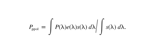
Table 2 lists values of the expected Pppol for a number of polarized standard stars we have observed.
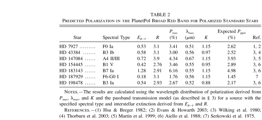 |
Observations of polarized standard stars are listed in Table 3, with integration times that are typically 4 minutes for each Stokes parameter. From this table, it can be seen that the observed polarizations are less than those predicted, by a factor that averages 0.986, which is ∼12% higher than the value based on the anticipated PEM modulation efficiency and the detector frequency responses. Therefore, two corrections are applied to the measured polarization values, in addition to those described in § 2.5. They need to be divided by a factor of 0.986 for the frequency response, and an additional factor (slightly color dependent) for the wavelength dependence of the PEM modulation as given in Table 1.
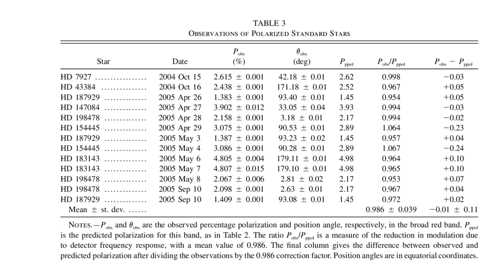 |
Once corrected, the differences between predicted and observed polarizations for the standard stars (final column of Table 3) have a standard deviation of 0.11%, and this drops to 0.04% if the one most discrepant point (HD 154445 on 2005 May 4) is omitted. In view of the quoted accuracies of the Pmax values (typically ∼0.05%) and the fact that there are indications of variability in these standards (Bastien et al. 1988), the agreement is excellent. The absolute accuracy of measuring polarization, by comparison with all the polarized standards, is 1.1%.
4.4. Nearby Bright Stars
Table 4 shows the polarization of a number of nearby bright stars (within 32 pc). The errors were calculated by comparing the two quantities E1 and E2 and quoting the larger one. The notation E1 is the standard error on the mean of qi and ui (calculated from the residuals of four to six separate observations to the TP fit described in § 4.1), with the uncertainty in the instrumental polarization added in quadrature. And E2 is the expected error on the mean of qi and ui, derived by adding in quadrature the contributions of the random errors (see § 2.5), the uncertainty in TP, and the uncertainty in instrumental polarization. It is preferable in principle to use E1 (which is based on the actual scatter in separate measurements and is usually the larger quantity; see § 4.1), but since the number of measurements is small, it is appropriate to use E2 in cases where E1 happens to be smaller. Note that in E2, the uncertainty in TP is taken to be the uncertainty in P/√2 (where P is the amplitude of the TP sine curve), since this is the typical contribution of TP to the error for our measurements, which sample the range of parallactic angles evenly.
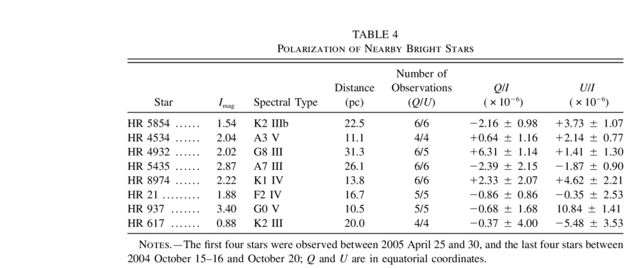 |
The polarizations measured for these nearby stars are very low (typically only a few ×10−6). This implies that both the interstellar and intrinsic polarizations are low. Extrapolation of the polarization‐distance relation for distant stars (e.g., Behr 1959) would imply polarizations of ∼2 × 10⁻⁴ at 10 pc and 6 × 10⁻⁴ at 30 pc. The results we have obtained are a factor of 100 lower than this, an indication of very low levels of dust in the local bubble around the Sun. The intrinsic linear polarizations of these stars (e.g., resulting from stellar activity) must also be low. A later paper will present results for a much larger sample of stars out to distances of ∼100 pc.
4.5. Integration Times
In practice, a random error of 1 × 10⁻⁶, as calculated by the reduction script from the noise in the detected signal, is achieved in a 390 s elapsed time, or 370 s integration time, for an I = 0 mag star on a 4 m telescope, with a filter passband of ∼320 nm. The expected performance can be calculated as follows. A total of 2 × 10¹² photons are required in order to reach 1 × 10⁻⁶ in fractional polarization (both Stokes parameters). Factoring in the telescope and PlanetPol throughput, the detector quantum efficiency, and the PEM modulation efficiency, we need a total of 6.6 × 10¹² photons incident on the telescope primary. An I = 0 mag star gives 8.2 × 10¹⁰ photons s−1 at the top of the atmosphere (WHT‐SIGNAL exposure time calculator) with a 140 nm passband, or 1.2 × 10¹¹ photons s−1 in the 320 nm PlanetPol passband, assuming a 90% atmospheric transmission for the I‐band and including the 0.7 WHT‐SIGNAL factor. Thus, a fractional polarization of 1 × 10⁻⁶ should be reached in ∼55 s for a 0 mag star, compared to 370 s in practice, i.e., a factor of ∼6.7 increase, or noise of ∼2.5. However, the calculation has not taken into account the well‐known additional noise that is produced in the avalanche process, which increases the photon noise by a factor that depends on the APD gain and is approximately 2 for the APDs we are using, close to the actual increase in noise of ∼(6.7)1/2, or ∼2.5. The random error calculated by the reduction script is inversely proportional to the square root of the detected stellar flux and the square root of the integration time for all measurements that we have made, for stars of 1–7 mag. This indicates that the performance of PlanetPol is photon‐noise–limited for individual measurements. As noted in § 4.1, the residuals to the TP fit for individual stars are on average 1.6–1.7 times larger than would be expected from the random errors, and this factor appears to be independent of stellar magnitude and the number of separate measurements. This suggests that the precision of polarization measurements with PlanetPol for nearby bright stars with very low polarizations can in principle be improved by repeated measurements in a photon‐noise–limited way, down to a limit in fractional polarization near 0.2 × 10⁻⁶ that is set by the 1.1% precision of the PlanetPol measurement of a TP of typically 2 × 10⁻⁶.
4.6. Efficacy of Measuring Polarizations of Parts per Million
As indicated in §§ 4.1 and 4.2, the telescope and instrument polarizations have to be measured for each observing run, although we have no evidence that either of these change during a run, the longest to date being seven nights. This does introduce a significant overhead, although this will be reduced as we gain confidence in the best low‐polarization stars to use (although we can never rule out intrinsic variability). Stars used to determine the TP have I magnitudes ranging from 0.9 to 3.4, but for each star, it typically takes 14 minutes of elapsed time to measure a single Stokes parameter. Assuming four stars are each measured five times, plus six further measurements are made with the instrument rotated to +90° and −45° to measure the IP, this gives a total of almost 11 hr for calibrations, or approximately one and a half nights, including acquisition overheads. To determine the polarization signature of the hot Jupiters with orbital periods of 3 or 4 days requires about seven nights in order to get adequate phase coverage so that calibrations represent about 20% of the total observing time.
5. ATMOSPHERIC CONDITIONS
Polarimetry is often regarded as being immune to atmospheric conditions, although observations of the Sun by Kemp et al. (1987), using apertures ranging from 15' to 2°, observed false polarization signals at large zenith distances, which is worst in the B band, and was attributed to double scattering by aerosols and molecules in the Earth's atmosphere. This will not be a problem with the PlanetPol observations, which are made with very much smaller apertures and at longer wavelengths. However, we have found that Saharan dust, not an uncommon occurrence on the island of La Palma in the summer months, can also produce polarization. The dust, consisting of large gray particles, can introduce a fractional polarization signal of ∼40 × 10−6 at a zenith distance of ∼40° when the dust reduces transmission at the zenith by ∼25% in the red. We attribute the dust polarization PD to dichroic extinction, and it appears to be a strong function of zenith distance ZD, declining to near zero for ZD < 20°. If the effect is due to dichroic extinction, we would expect that PD = C(1 - cos ZD) (C being a function mainly of dust column density), and the data appear to bear this out, although analysis is currently at an early stage. Hence, it should be possible to minimize this effect when it occurs by observing science targets only near the zenith [reducing the effect to (1–4) × 10−6] and subtracting the calculated PD. One difficulty is that the parameter C is likely to have some temporal and directional variability, even within each night, so the error bars on any data of very bright stars will be noticeably increased. However, for the brightest planetary systems, the uncertainty in PD when observing near the zenith is less than the shot noise, so the effect on the overall errors is minimal. A more detailed analysis of the effect of Saharan dust will appear in a later paper (J. A. Bailey et al. 2006, in preparation).
It is known from lidar measurements that specific orientation of ice particles must exist in some cirrus clouds (Liou 2002), and thus we might expect to see polarization produced by cirrus clouds, although to date we have no clear evidence for this. We have found that data taken for low‐polarization stars during conditions of thick clouds (50% or more reduction in throughput) are more likely to deviate from expected values by >1.5 σ than data taken in clear weather or through thin clouds (even allowing for the appropriate larger σ for reduced throughput). The reason for this is unclear, but we recommend that very high precision measurements not be attempted under such conditions.
6. SCIENCE PROGRAMS
To date, PlanetPol has been used mainly to determine the polarization of extrasolar planets, and some preliminary data for τ Bootis are published in Hough et al. (2006). A more complete data set for τ Boo will appear in a separate paper (P. W. Lucas et al. 2006, in preparation). In addition, a program to determine the distribution of dust in the local solar environment by measuring the polarization of stars at distances up to 100 pc is being carried out (see § 4.4), and we have also observed stars with debris disks or very high rotation rates that can produce polarization by electron scattering in a highly flattened stellar atmosphere.
7. CONCLUSIONS AND FUTURE DEVELOPMENTS
We have constructed and successfully commissioned a photopolarimeter, PlanetPol, that is capable of achieving fractional polarization sensitivities of 10−6 when used at the unfolded Cassegrain focus of the William Herschel Telescope, with an absolute accuracy, as determined from observations of classical polarized standards, of ∼1%. This is the first time such high sensitivities have been achieved on a conventional telescope, and it provides a number of new scientific opportunities.
Particular care has been taken to identify and compensate for systematic effects, foremost of which are electronic offsets that are readily removed by rotating the analyzer through 90° with respect to the modulator, thereby changing the polarity of the signals. Additional small offsets in the modulated signal that are proportional to the flux from the star and are at a level of a few parts per million can be effectively removed so that their contribution is below the shot noise. Their origin is unclear.
As PlanetPol is limited solely by the number of photons, it would benefit from being used on larger telescopes, such as the present 8 and 10 m class telescopes and the future Extremely Large Telescopes, although avoiding oblique reflections will always be important in attaining the highest polarization sensitivities. We have observed that Saharan dust can produce additional polarization that detracts from the usual claim that polarimetry is independent of atmospheric conditions.
The performance of PlanetPol is currently limited by excess noise associated with APDs that effectively increases the photon shot noise. With the very high photon count rates, it is not possible to perform photon counts, and photodiode amplifiers, with the bandwidth needed when used with PEMs, do not outperform APDs. One possible approach would be to use ferroelectric liquid crystals as the polarization modulator. These can operate at frequencies of ∼1 kHz (or less), still sufficient to remove most atmospheric effects, making it easier to use photodiodes with the lower bandwidths. It should be emphasized, however, that it has not been demonstrated that FLCs can achieve the same very high polarization sensitivities as PEMs.
We acknowledge the award of a grant from the Particle Physics and Astronomy Research Council to build the polarimeter. We are grateful to the staff of the William Herschel Telescope, La Palma, for the excellent support we have received. We thank an anonymous referee for a number of useful suggestions.
APPENDIX A: DERIVATION OF THE THEORETICAL POLARIZATION EFFICIENCY
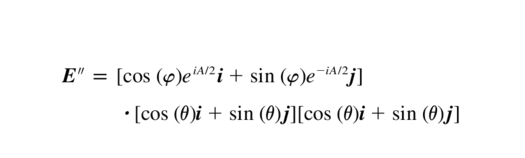
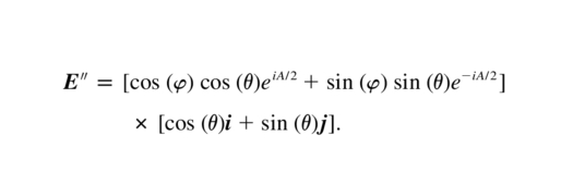
Here we derive the theoretical polarization efficiency of an optical system consisting of a PEM and analyzer and evaluate the result for a half‐wavelength retardance amplitude, generalizing the formulae given by J. C. Kemp (1987, unpublished)6 for a specific position angle of polarization. We define two angles relative to the fast axis of the PEM: θ is the orientation of the analyzer (θ = ± 45° for the two beams emerging from the PlanetPol Wollaston prisms), and φ is the orientation of the plane of the polarization of the incident beam, which is assumed to be partially linearly polarized with polarization fraction PL. Following J. C. Kemp (1987, unpublished), we define a unit vector in the plane of the PEM fast axis as i , and that in the slow axis as j . Adapting from J. C. Kemp (1987, unpublished), the electric vector of the linearly polarized component of the incident wave, after passing through the PEM, is given by

where A is the instantaneous value of the PEM retardance in radians, and we have neglected the usual e−iωt factor. After passing through the analyzer, the electric vector is obtained by projecting E' onto the plane of the analyzer, using a scalar product of E' with the unit vector, to give the amplitude
or
The output intensity of the beam produced by the linearly polarized component of the incident light is then given by
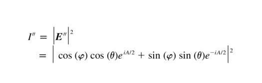
or
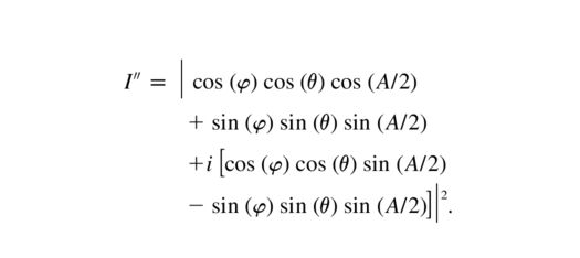
After expanding, rearranging, and using common trigonometric identities, this becomes
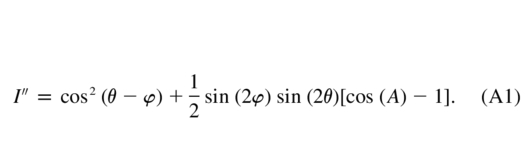
We define A = A0cos (ω1t) for PEM retardance at angular frequency ω1 and then use the identity
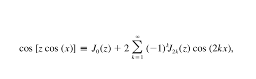
where Jn(z) is a Bessel function.
Therefore,
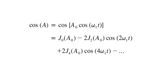
The modulated signal is extracted by lock‐in amplifiers tuned to the oscillation at angular frequency 2ω1, and is output as the rms value. We define the ratio of the rms modulated signal to the DC signal in each emerging beam as Pmeas. For the case of very low polarization, we can assume that the constant terms in equation (A1) are negligible compared to the DC flux, which will be dominated by unpolarized light. So
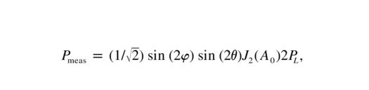
where the final factor of 2 comes from dividing the DC flux into two beams assumed to have equal intensity.
Operating at half‐wave retardance amplitude, we have J2(π) = 0.486. Since we set θ = ± 45° for the two beams, sin (2 θ) = ± 1. Hence,

Hence, the theoretical efficiency factor when measuring very weakly polarized light is 0.687. The sin (2ϕ) factor indicates the need for two measurements taken with the instrument rotated by 45° in order to measure Stokes Q and U. Note that for calculations of the expected shot noise, the efficiency factor is slightly different, since the detected polarized flux is proportional to the average value of |cos (2ω1t)|, which is 2/π = 0.637 when integrated over a whole number of cycles. This is less than the usual rms factor of 1/√2 = 0.707 that was used in the above calculation and yields an efficiency factor of 0.619.
For the case in which the incident light has a significant polarization, we must add the DC flux terms from equation (A1) into the calculation of Pmeas:
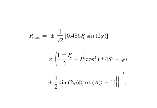
where 〈cos (A)〉 denotes the time‐averaged value of cos (A). All the oscillating terms in the expansion of 〈cos (A)〉 average to zero over time, so at half‐wave retardance amplitude, we have A0 = π and 〈cos (A)〉 = J0(π) = -0.3042.
This yields
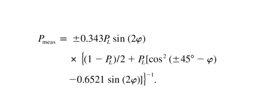
Using common trigonometric identities, we find cos2(± 45° - ϕ)≡1/2 ± 1/2sin (2ϕ). This leads to
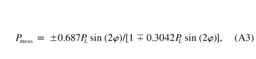
where the plus signs correspond to θ = 45° and the minus signs correspond to θ = -45°. This then equates to the precise equation for P1 given near the end of § 2.5, where we use Q/I or U/I to represent PLsin (2ϕ), depending on the orientation of the instrument.
APPENDIX B: DATA FITTING AND THE GAUSS‐NEWTON METHOD
Suppose we have a set of observations θ1,..., θm at times t1,...,tm and that we believe there is an underlying model

where x1,...,xn are model parameters to be determined. The least‐squares approach calculates these parameters by minimizing the sum of squares of residuals

that is, by minimizing
Such problems are relatively easy to solve when φ is a linear function of the parameters; e.g., when φ is a polynomial and
The Gauss‐Newton method is designed to deal with problems of the form given in equation (B1) for more complicated models in which φ is a nonlinear function of the parameters x, such as

The Gauss‐Newton method uses the fact that

and
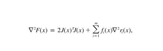
where r(x) = [r1(x),...,rm(x)]T and J(x) is the Jacobian matrix whose (i, j)‐th element is ∂ri(x)/∂xj. If the minimum value of F is near zero and/or the residuals ri are near linear, the second term in ∇2F(x) can be neglected, and hence the iteration
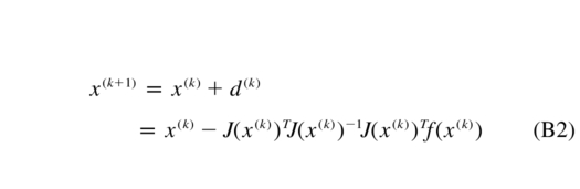
can be regarded as an approximate form of the Newton method for minimizing F(x). Practical implementations of the algorithm include a line search so that x(k + 1) = x(k) + αd(k), where α is a scalar chosen to ensure F(x(k + 1))<F(x(k)).
Footnotes
- 6
In "Polarized Light and Its Interaction with Modulation Devices" (Hinds International, Inc.)