When multiple variables are associated with a response, the interpretation of a prediction equation is seldom simple.
Last month we explored how to model a simple relationship between two variables, such as the dependence of weight on height1. In the more realistic scenario of dependence on several variables, we can use multiple linear regression (MLR). Although MLR is similar to linear regression, the interpretation of MLR correlation coefficients is confounded by the way in which the predictor variables relate to one another.
In simple linear regression1, we model how the mean of variable Y depends linearly on the value of a predictor variable X; this relationship is expressed as the conditional expectation E(Y|X) = β0 + β1X. For more than one predictor variable X1, . . ., Xp, this becomes β0 + ΣβjXj. As for simple linear regression, one can use the least-squares estimator (LSE) to determine estimates bj of the βj regression parameters by minimizing the residual sum of squares, SSE = Σ(yi − ŷi)2, where ŷi = b0 + Σjbjxij. When we use the regression sum of squares, SSR = Σ(ŷi − Y−)2, the ratio R2 = SSR/(SSR + SSE) is the amount of variation explained by the regression model and in multiple regression is called the coefficient of determination.
The slope βj is the change in Y if predictor j is changed by one unit and others are held constant. When normality and independence assumptions are fulfilled, we can test whether any (or all) of the slopes are zero using a t-test (or regression F-test). Although the interpretation of βj seems to be identical to its interpretation in the simple linear regression model, the innocuous phrase “and others are held constant” turns out to have profound implications.
To illustrate MLR—and some of its perils—here we simulate predicting the weight (W, in kilograms) of adult males from their height (H, in centimeters) and their maximum jump height (J, in centimeters). We use a model similar to that presented in our previous column1, but we now include the effect of J as E(W|H,J) = βHH + βJJ + β0 + ε, with βH = 0.7, βJ = −0.08, β0 = −46.5 and normally distributed noise ε with zero mean and σ = 1 (Table 1). We set βJ negative because we expect a negative correlation between W and J when height is held constant (i.e., among men of the same height, lighter men will tend to jump higher). For this example we simulated a sample of size n = 40 with H and J normally distributed with means of 165 cm (σ = 3) and 50 cm (σ = 12.5), respectively.
Although the statistical theory for MLR seems similar to that for simple linear regression, the interpretation of the results is much more complex. Problems in interpretation arise entirely as a result of the sample correlation2 among the predictors. We do, in fact, expect a positive correlation between H and J—tall men will tend to jump higher than short ones. To illustrate how this correlation can affect the results, we generated values using the model for weight with samples of J and H with different amounts of correlation.
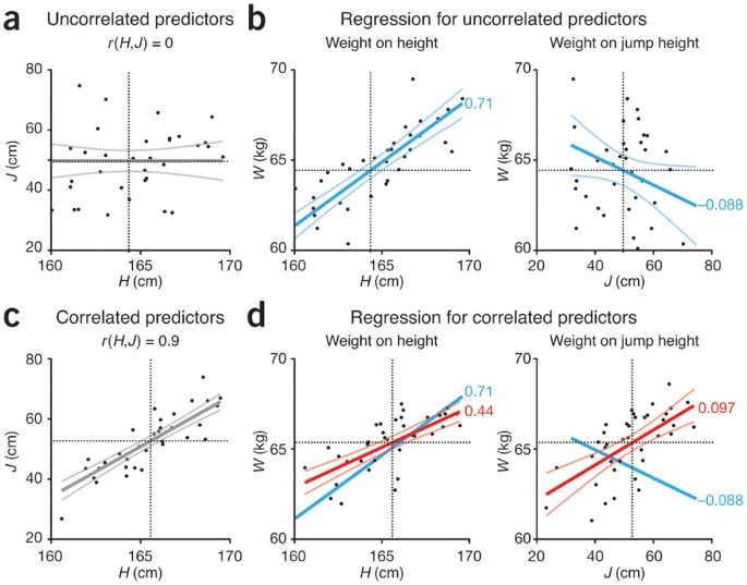
Let's look first at the regression coefficients estimated when the predictors are uncorrelated, r(H,J) = 0, as evidenced by the zero slope in association between H and J (Fig. 1a). Here r is the Pearson correlation coefficient2. If we ignore the effect of J and regress W on H, we find Ŵ = 0.71H − 51.7 (R2 = 0.66) (Table 1 and Fig. 1b). Ignoring H, we find Ŵ = −0.088J + 69.3 (R2 = 0.19). If both predictors are fitted in the regression, we obtain Ŵ = 0.71H − 0.088J − 47.3 (R2 = 0.85). This regression fit is a plane in three dimensions (H, J, W) and is not shown in Figure 1. In all three cases, the results of the F-test for zero slopes show high significance (P ≤ 0.005).
(a) Simulated values of uncorrelated predictors, r(H,J) = 0. The thick gray line is the regression line, and thin gray lines show the 95% confidence interval of the fit. (b) Regression of weight (W) on height (H) and of weight on jump height (J) for uncorrelated predictors shown in a. Regression slopes are shown (bH = 0.71, bJ = −0.088). (c) Simulated values of correlated predictors, r(H,J) = 0.9. Regression and 95% confidence interval are denoted as in a. (d) Regression (red lines) using correlated predictors shown in c. Light red lines denote the 95% confidence interval. Notice that bJ = 0.097 is now positive. The regression line from b is shown in blue. In all graphs, horizontal and vertical dotted lines show average values.
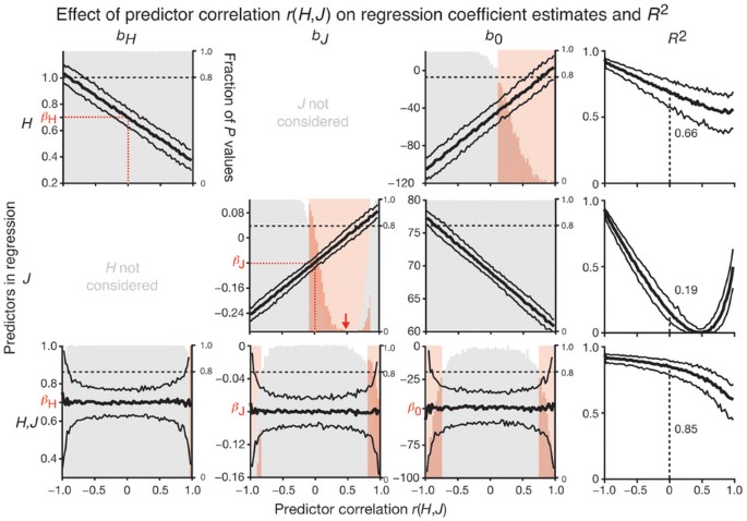
When the sample correlations of the predictors are exactly zero, the regression slopes (bH and bJ) for the “one predictor at a time” regressions and the multiple regression are identical, and the simple regression R2 sums to multiple regression R2 (0.66 + 0.19 = 0.85; Fig. 2). The intercept changes when we add a predictor with a nonzero mean to satisfy the constraint that the least-squares regression line goes through the sample means, which is always true when the regression model includes an intercept.
Shown are the values of regression coefficient estimates (bH, bJ, b0) and R2 and the significance of the test used to determine whether the coefficient is zero from 250 simulations at each value of predictor sample correlation −1 < r(H,J) < 1 for each scenario where either H or J or both H and J predictors are fitted in the regression. Thick and thin black curves show the coefficient estimate median and the boundaries of the 10th–90th percentile range, respectively. Histograms show the fraction of estimated P values in different significance ranges, and correlation intervals are highlighted in red where >20% of the P values are >0.01. Actual regression coefficients (βH, βJ, β0) are marked on vertical axes. The decrease in significance for bJ when jump height is the only predictor and r(H,J) is moderate (red arrow) is due to insufficient statistical power (bJ is close to zero). When predictors are uncorrelated, r(H,J) = 0, R2 of individual regressions sum to R2 of multiple regression (0.66 + 0.19 = 0.85). Panels are organized to correspond to Table 1, which shows estimates of a single trial at two different predictor correlations.
Balanced factorial experiments show a sample correlation of zero among the predictors when their levels have been fixed. For example, we might fix three heights and three jump heights and select two men representative of each combination, for a total of 18 subjects to be weighed. But if we select the samples and then measure the predictors and response, the predictors are unlikely to have zero correlation.
When we simulate highly correlated predictors r(H,J) = 0.9 (Fig. 1c), we find that the regression parameters change depending on whether we use one or both predictors (Table 1 and Fig. 1d). If we consider only the effect of H, the coefficient βH = 0.7 is inaccurately estimated as bH = 0.44. If we include only J, we estimate βJ = −0.08 inaccurately, and even with the wrong sign (bJ = 0.097). When we use both predictors, the estimates are quite close to the actual coefficients (bH = 0.63, bJ = −0.056).
In fact, as the correlation between predictors r(H,J) changes, the estimates of the slopes (bH, bJ) and intercept (b0) vary greatly when only one predictor is fitted. We show the effects of this variation for all values of predictor correlation (both positive and negative) across 250 trials at each value (Fig. 2). We include negative correlation because although J and H are likely to be positively correlated, other scenarios might use negatively correlated predictors (e.g., lung capacity and smoking habits). For example, if we include only H in the regression and ignore the effect of J, bH steadily decreases from about 1 to 0.35 as r(H,J) increases. Why is this? For a given height, larger values of J (an indicator of fitness) are associated with lower weight. If J and H are negatively correlated, as J increases, H decreases, and both changes result in a lower value of W. Conversely, as J decreases, H increases, and thus W increases. If we use only H as a predictor, J is lurking in the background, depressing W at low values of H and enhancing W at high levels of H, so that the effect of H is overestimated (bH increases). The opposite effect occurs when J and H are positively correlated. A similar effect occurs for bJ, which increases in magnitude (becomes more negative) when J and H are negatively correlated. Supplementary Figure 1 shows the effect of correlation when both regression coefficients are positive.
When both predictors are fitted (Fig. 2), the regression coefficient estimates (bH, bJ, b0) are centered at the actual coefficients (βH, βJ, β0) with the correct sign and magnitude regardless of the correlation of the predictors. However, the standard error in the estimates steadily increases as the absolute value of the predictor correlation increases.
Neglecting important predictors has implications not only for R2, which is a measure of the predictive power of the regression, but also for interpretation of the regression coefficients. Unconsidered variables that may have a strong effect on the estimated regression coefficients are sometimes called 'lurking variables'. For example, muscle mass might be a lurking variable with a causal effect on both body weight and jump height. The results and interpretation of the regression will also change if other predictors are added.
Given that missing predictors can affect the regression, should we try to include as many predictors as possible? No, for three reasons. First, any correlation among predictors will increase the standard error of the estimated regression coefficients. Second, having more slope parameters in our model will reduce interpretability and cause problems with multiple testing. Third, the model may suffer from overfitting. As the number of predictors approaches the sample size, we begin fitting the model to the noise. As a result, we may seem to have a very good fit to the data but still make poor predictions.
MLR is powerful for incorporating many predictors and for estimating the effects of a predictor on the response in the presence of other covariates. However, the estimated regression coefficients depend on the predictors in the model, and they can be quite variable when the predictors are correlated. Accurate prediction of the response is not an indication that regression slopes reflect the true relationship between the predictors and the response.
References
Altman, N. & Krzywinski, M. Nat. Methods 12, 999–1000 (2015).
Altman, N. & Krzywinski, M. Nat. Methods 12, 899–900 (2015).
Author information
Authors and Affiliations
Ethics declarations
Competing interests
The authors declare no competing financial interests.
Integrated supplementary information
Supplementary Figure 1 Regression coefficients and R2
The significance and value of regression coefficients and R2 for a model with both regression coefficients positive, E(W|H,J) = 0.7H + 0.08J - 46.5 + ε. The format of the figure is the same as that of Figure 2.
Supplementary information
Supplementary Figure 1
Regression coefficients and R2 (PDF 299 kb)
Rights and permissions
About this article
Cite this article
Krzywinski, M., Altman, N. Multiple linear regression. Nat Methods 12, 1103–1104 (2015). https://doi.org/10.1038/nmeth.3665
Published:
Issue Date:
DOI: https://doi.org/10.1038/nmeth.3665
This article is cited by
-
Income and Oral and General Health-Related Quality of Life: The Modifying Effect of Sense of Coherence, Findings of a Cross-Sectional Study
Applied Research in Quality of Life (2023)
-
Outcomes of a novel all-inside arthroscopic anterior talofibular ligament repair for chronic ankle instability
International Orthopaedics (2023)
-
Predicting financial losses due to apartment construction accidents utilizing deep learning techniques
Scientific Reports (2022)
-
Regression modeling of time-to-event data with censoring
Nature Methods (2022)
-
A Systematic Analysis for Energy Performance Predictions in Residential Buildings Using Ensemble Learning
Arabian Journal for Science and Engineering (2021)


