


Introduction
At times of low sea level during the glacial periods of the Pleistocene, the North Sea area (Fig. 1) formed a highly suitable environment for hunter-gatherers. Expansive coastal lowlands supported abundant game for hunting, and coastal and shallow-marine waters offered opportunities for fishing (Coles, Reference Coles1998). Tens of thousands of mammal remains retrieved as by-products of modern fishing, dredging and aggregate extraction are testament to the fact that these drowned landscapes were favourable to human occupation and possibly even preferred in comparison to adjacent higher areas represented by modern ‘dry land’ (Gaffney et al., Reference Gaffney, Fitch and Smith2009).
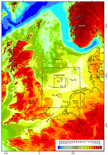
Fig. 1. North Sea area and outline of areas depicted in other figures. The edge of the continental shelf, and thus of the partially to fully emerged lowland during lowstands, is shown as the transition from dark to light blue in this merged image of bathymetry (http://www.emodnet-hydrography.eu) and topography (http://www.ngdc.noaa.gov/mgg/global/global.html; Amante & Eakins, Reference Amante and Eakins2009) in metres above or below sea level. Towards the present-day upland, colours change from blue via green and yellow to red and brown.
However, the complexity of these drowned landscapes has not been captured by traditional geological maps of the North Sea subsurface, which to date have formed the main source of information for palaeolandscape reconstructions. Such maps, which are based on geophysical, core and palaeoenvironmental data, merely provide an overview of the Pleistocene and Holocene geology of the North Sea. When combined with local and regional analyses of sea-level and ice-sheet dynamics, they also contribute to our understanding of the process–response relationships that have governed the evolution of the North Sea Basin. The associated data-acquisition strategy, developed for mapping at a 1:250,000 scale, does not meet the resolution requirements of detailed palaeolandscape reconstructions (Fig. 2). The density of seismic and core data may be sufficient to provide clues with respect to the overall archaeological setting and potential, but it is commonly not high enough to map the distribution of depositional environments, which are key building blocks for palaeolandscape reconstructions. The density of bathymetric data is usually much higher, but bathymetry can only provide information on the top horizon of the vertical succession that has recorded the landscape history. Additionally, bathymetry does not usually represent a single well-preserved landscape; rather, it shows a patchwork of landscape elements that reflect temporally and laterally variable episodes of erosion and deposition (Fitch et al., Reference Fitch, Thomson and Gaffney2005).
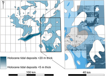
Fig. 2. Comparison between a traditional map showing the distribution of fine-grained Holocene tidal deposits (left) and a time slice of 3D seismic data (right). The traditional map only provides coarse information on buried palaeolandscapes. In contrast, the time slice shows that the Holocene tidal deposits are characterised by a complex and detailed fill pattern, allowing derivation of drainage directions (and therefore providing information on the palaeocoastline). The dashed line marks the boundary between UK and Dutch waters.
Current state-of-the-art mapping approaches aim at optimising data density, either through new data acquisition or through use of existing full-coverage seismics acquired during the past decades for the hydrocarbon industry. Such 3D seismics were first used for landscape reconstruction by Fitch et al. (Reference Fitch, Thomson and Gaffney2005). Here, we provide an overview of high-definition reconstructions of landscapes preserved in the shallow subsurface (upper tens to hundreds of metres of sediment) of the North Sea from an archaeological perspective. Although far from complete, detailed landscape reconstructions have been made for large areas of the North Sea, with a focus on the Late Glacial and early Holocene.
Owing to a great improvement in resolution (Fig. 2), these new reconstructions provide part of the environmental context for the entire Quaternary Period, which is needed by archaeologists to shed light on Palaeolithic, Mesolithic and Neolithic societies in an analytical approach akin to habitat-suitability studies that have provided a major impulse to seabed-habitat mapping and modelling during the past decade (e.g. Degraer et al., Reference Degraer, Verfaillie, Willems, Adriaens, Vincx and Van Lancker2008). Although early humans can obviously not be compared directly to benthic or pelagic organisms, their dependence on and strategic use of large-scale landscapes and smaller-scale landscape niches makes palaeolandscape a suitable and promising proxy for potential human land use and settlement. By analysing the palaeolandscape record, abundant and much-needed information is added to relatively rare archaeological North Sea finds. Together, they will not necessarily tell the same story as the onshore evidence from the surrounding countries (Peeters et al., Reference Peeters, Murphy and Flemming2009).
Over the last 10 years, blurred and commonly variable representations offered by traditional mapping products have been replaced by much more accurate versions. For an increasing number of generally sizable areas, these new palaeogeographic maps offer detail relating to some of the most influential climate- and sea-level-related landscape changes that have affected and been used by human societies in northwestern Europe (Leary, Reference Leary2009). A key challenge within this area concerns the identification and mapping of interglacial landscape elements from before the last glaciation in those places where they have been preserved. Given the future goal of full palaeolandscape mapping and reconstruction, targeted research is required to ensure the optimum use of all high-definition windows and to guide further surveys in a manner that can enable and improve feature identification and contribute significantly to the solution of key archaeological questions.
Seismic methods
Equipment
In marine seismic-reflection surveys, sound waves generated by a seismic source towed by or mounted on a vessel are used to obtain information on the subsurface (Fig. 3a). Seismic waves travel through water and sediment at velocities of 1500–2000 m s–1. When a seismic wave encounters a boundary between two materials with different acoustic properties, some of the energy in the wave will be reflected at the boundary. The remaining energy will pass through the boundary and continue downward. The amplitude of the reflected wave depends on the impedance contrast between the two materials. This contrast, a function of velocity differences at boundaries, is greatest at the water–seabed interface. Reflected waves are recorded using hydrophones that convert pressure changes into electrical signals or, in chirp systems, by the transducers that also generate the outgoing signal. The receivers record the time it takes for a sound wave to travel from the source to a particular boundary and back. If the seismic wave velocities through the water column and in the subsurface sediment are known, this so-called two-way travel time (TWTT) may be used to calculate the depth to reflecting boundaries.

Fig. 3. Acquisition methodology of 3D seismic data. A vessel tows a seismic source and a series of parallel streamers along a transect a. The signal produced by the moving source is reflected at the seabed and at boundaries between subsurface units, and the reflected signals are recorded by hydrophones in the streamers. Techniques to process the raw signal include migration b. and stacking c. Signals and ship and source positions for times 1, 2 and 3 are colour-coded in blue, green and red.
A distinction can be made between high-resolution single- or multi-channel systems using frequencies of 100–10,000 Hz and low-resolution multi-channel systems using <100 Hz (Table 1). High-frequency single-channel systems record through short hydrophones. Their vertical resolution is in the order of 0.1 m to a few metres, depending on the frequency used. Disadvantages are quality loss below the first seabed multiple, which is a problem in shallow water, and reduced vertical resolution by unprocessed multiple noise below depths of 100 ms (c. 75 m, including the water column). Furthermore, multiple noise and mismatches between relatively large wavelengths of the source signal and the typically smaller-scale lamination and bedding in stratigraphic units may result in chaotic configurations rather than consistent composite reflections. High-frequency multi-channel systems record through hydrophone arrays in cables (streamers). Vertical resolution for these systems is in the order of a few metres below 100 ms, but this can be lower for shorter TWTT because of near-source effects.
Table 1 Overview of the most frequently used seismic systems and their characteristics (after Praeg, Reference Praeg2003).
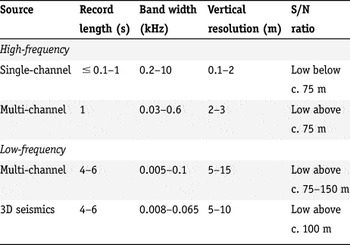
Low-frequency multi-channel systems record the reflected signal through kilometre-long hydrophone arrays. Complex intervals of differing acoustic facies are turned into single composite reflections. Vertical resolution is 5–15 m, depending not only on the frequency but also on survey and source characteristics in relation to the geometry of subsurface units and on post-survey processing (Praeg, Reference Praeg2003). Horizontal resolution is lower than vertical resolution (Sheriff, Reference Sheriff, Berg and Woolverton1985). For any frequency, the best resolution is reached when survey lines are closely spaced and when the subsurface is characterised by well-defined, gently dipping lithological interfaces that are laterally continuous. In general, information on the upper 100–200 ms is distorted and ambiguous as a result of a shift to lower frequencies that increases with proximity of source to subsurface target. When acquisition parameters, such as the separation between source and nearest-offset receiver, and processing are optimised for the shallow subsurface, information may be obtained from 50 ms downwards (Sheriff, Reference Sheriff, Berg and Woolverton1985). When water depth is about 40 m or more, features at or near the seabed may be imaged. Below 150–200 ms, information is commonly superior to that from high-frequency profiles.
In 3D surveys, multiple streamers are deployed in a closely spaced parallel configuration to record data suitable for 3D interpretation of subsurface units. Streamer spacing as narrow as 12.5 m is frequently achieved, with new high-density 3D systems offering the prospect of even closer streamer spacing. Most 3D surveys employ low-frequency systems, which work best in deeper waters and cover very large areas efficiently at a coarse vertical resolution (Fitch et al., Reference Fitch, Thomson and Gaffney2005). Although high-resolution 3D seismic systems are available, areal coverage is currently too limited to enable regional palaeolandscape reconstructions. Moreover, these systems are commonly hampered by source instability (cf. Müller et al., Reference Müller, Milkereit, Bohlen and Theilen2002).
Processing and interpretation
Important signal-processing techniques are deconvolution, stacking and migration. Deconvolution or inverse filtering corrects for sound-wave deformation as seismic energy is filtered by the subsurface. It helps to recover detailed high-frequency information, evens out amplitudes and reduces multiples. Migration relocates reflections created by narrow or steep subsurface features from their recorded to their actual positions (Fig. 3b). Stacking transforms traces from different shot records with a common reflection point (in multi-channel surveys) into a single trace to improve the signal-to-noise ratio (Fig. 3c).
After processing, seismic attributes (including amplitude, dip, frequency and polarity) may be analysed to reconstruct sedimentary sequences (vertically) or map depositional systems (laterally).
Seismic profiles, time slices and horizon slices
Data collected via a single cable or streamer are displayed as vertical cross-sections through the subsurface (Fig. 4a). In most traditional surveys conducted by the British, Dutch and Belgian geological surveys for North Sea mapping purposes, distances between adjacent profiles are in the order of 10 km or more (cf. Cameron et al., Reference Cameron, Laban and Schüttenhelm1984). Such a wide spacing is usually sufficient to understand the overall architecture and formation of large-scale sedimentary systems, but makes it difficult to carry out detailed landscape reconstructions. Not all reflections can be correlated among lines, and most landscape elements have lateral dimensions smaller than can be resolved in a 10 × 10 km grid.

Fig. 4. Three examples of processed seismic data and their visualisation. a. High-frequency seismic profile showing late-Pleistocene river dunes offshore from the western Netherlands coast, buried under a sequence of Holocene coastal and marine deposits. b. Time slice from post-processed 3D seismics showing various early Holocene channel fills in the Oyster Grounds area on the Netherlands Continental Shelf. c. Relief-shaded horizon slice of Pleistocene tunnel valleys near the Western Mudhole on the Netherlands Continental Shelf.
Data collected with multiple parallel streamers may be displayed as vertical cross-sections, time slices (Fig. 4b) or horizon slices (Fig. 4c). Time slices are sections of 3D seismic data with a certain uniform arrival time. Because of the spatial variability of sound velocity in the subsurface, they are near-horizontal rather than perfectly horizontal depth slices. Their map view makes time slices very suitable for the identification of landscape elements as reflected in seismic amplitude. Horizon slices show the spatial pattern of particular reflections, created by tracing these reflections on all survey lines and interpolating the resulting data. As reflections may be considered time horizons, regionally continuous or near-continuous reflections may represent palaeosurfaces relevant to palaeolandscape reconstruction. Thus, features can be extracted not only in planform but also in 3D, providing depth (and relative age) relationships.
Although low-frequency bandwidth is not necessarily a limiting factor in the analysis of low-frequency 3D seismic data because of compensation by spatial sampling (Praeg, Reference Praeg2003), features at or near the seabed in shallow water (<50 m) are poorly resolved. By using multiples in time slicing, such very shallow features may nevertheless be delineated (Fitch et al., Reference Fitch, Thomson and Gaffney2005). They are commonly better defined below the first seabed multiple, obscuring reflections from deeper features. To enhance the features seen in time slices, 3D seismic data may be converted into voxel (3D volume pixel) volumes, with each voxel containing the information from the original survey along with additional user-defined variables that may be visualised to facilitate interpretation. Units with seismic characteristics different from those of the surrounding area can be highlighted as opaque 3D shapes in a transparent space (Fitch et al., Reference Fitch, Thomson and Gaffney2005).
Accuracy of positioning
When comparing and combining different seismic data and cores, interpreters must be aware of the fact that positioning accuracy has improved steadily through time. In the 1950s, typical accuracies associated with the Decca Lo-Fix and LORAN-C systems were in the order of several hundreds of metres, especially far from the coast. Development of the Decca Hi-Fix and Hyper-Fix systems in the 1960s and 1980s, respectively, improved the accuracy by an order of magnitude. Introduction of public satellite-based global positioning systems in the 1990s, originally developed by and for the US military, marked the start of a further improvement in positioning. Originally, intentional degradation of GPS signals for civilian use limited the accuracy to far below its technical capabilities, spurring the development of the Differential Global Positioning System (DGPS) that uses a network of fixed, ground-based reference stations in addition to satellites. Even after intentional signal degradation was discontinued in 2000, DGPS has continued to improve location accuracy, which is now within 1 m. Lateral mismatches between features identified on seismic data or in cores are primarily the result of positioning issues. Vertical mismatches may be caused by insufficient correction for differences in water level, especially in areas marked by large tidal ranges, or instrument depth during data acquisition. Lateral mismatches are largest far from shore, whereas vertical mismatches are most significant in shallow near-coastal waters, where tidal amplification is common and instrument depth needs to be adjusted regularly to ensure optimal data quality (instrument as close to seabed as possible) while avoiding grounding-related damage.
Geologic and archaeological setting
As an area of long-term subsidence, much of the North Sea region provides excellent conditions for the preservation of glacial and interglacial deposits and landscapes. Evidence of multiple Pleistocene glaciations and deglaciations and of multiple regressions and transgressions is buried and stored in the subsurface. The geological record contains vestiges of the Pleistocene and Holocene landscape evolution as partly buried and erosive morphology, and shows a dominant influence of the Baltic river system early on, and of the shifting rivers Rhine, Meuse and Thames in later times. In the north, towards the centre of the North Sea Basin, subsidence during the Pleistocene has created the accommodation space for a thick stacked record of fluvial sediments with minor but useful markers of coastal, marine and glaciogenic deposits. Here, landscapes present at the time of the earliest human occupation are buried beneath hundreds of metres of sediment. In the south, towards the Strait of Dover, a near-absence of subsidence has resulted in the periodic reworking of sediment, resulting in multiple and compound lag deposits that contain a mixture of artefacts and mammalian fauna from different ages (Hijma et al., Reference Hijma, Cohen, Roebroeks, Westerhoff and Busschers2012). Here, only fragments and indirect indicators of palaeolandscapes have been preserved, such as the fill of an Eemian estuary offshore from Ostend in Belgium (Mathys, Reference Mathys2009).
Each palaeolandscape consists of smaller building blocks that represent the contribution of individual sedimentary environments. The main glacial and periglacial landscape features to be identified using seismic data are glacial depositional features (till plains, eskers, kames), glacial erosive features (tunnel valleys, tongue basins, iceberg scour marks), ice-marginal depositional features (ice-pushed ridges, outwash deltas, ice-marginal fans, sandur), proglacial lakes, pro- and periglacial rivers, and periglacial interfluves (coversand and loess plains). The main interglacial landscape features are offshore seabed (inner shelves, sand waves, tidal ridges, wave-formed lags), coastal depositional features (prograding shorefaces, barriers, tidal-basin fills, deltas, tidal-inlet fills, estuarine fills) and coastal erosive features (receding shorefaces, bluffs, islands (excluding barrier islands), estuarine re-entrants). These features may be partially or entirely preserved, and visible on seismic data, providing an incomplete record of multiple landscape generations from pre-glacial times onwards (Cohen et al., Reference Cohen, Gibbard and Weerts2014).
Seismic data as a source for palaeolandscape reconstruction
Scales and data spacing
The scale at which landscape elements can be recognised depends not only on the size of the elements, but also on the spacing of data such as cores, bathymetric measurements, and seismic lines and time slices (Fig. 5). In the past, combinations of typically widely spaced seismic lines and cores (few of which reach deeper than 10 m) resulted in maps on which only the largest landscape elements (multiple tens of kilometres) were recognisable. Although useful in providing the overall environmental setting of human occupation of the North Sea region in glacial and interglacial times, they cannot provide the detail needed to reconstruct palaeolandscapes accurately. For palaeolandscape mapping, features with spatial scales in the order of 1 km must be identifiable. In recent years, densely spaced 2D seismic grids or lines, particularly near the coast, and 3D seismic time slices have allowed such high resolution for more and more parts of the North Sea, increasing our insight into the glacial and interglacial palaeolandscapes that hosted man through time.
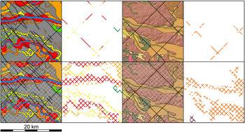
Fig. 5. Influence of the spacing of (2D) seismic lines on the accuracy of palaeolandscape reconstruction. Imaginary seismic grids of different densities (10 × 10 and 1 × 1 km) are projected on a typical fragment from a geomorphological map of a Dutch river-dominated landscape (left panels; Berendsen & Stouthamer, Reference Berendsen and Stouthamer2000) and a new geomorphological map of a Danish glacially dominated landscape (right panels; GEUS, unpublished data). Coarse grids traditionally used in marine mapping of the shallow subsurface provide little information on kilometre-scale landscape elements. Accurate interpolation between adjacent seismic profiles is generally not possible. Finer grids are much more suitable to reconstruct palaeolandscapes, although the lateral accuracy of such reconstructions is still inferior to that of 3D time slices or onshore geomorphological mapping. Boyd et al. (Reference Boyd, Coggan, Birchenough, Limpenny, Eastwood, Foster-Smith, Philpott, Meadows, James, Vanstaen, Soussi and Rogers2006) showed a similar effect of line spacing in seabed-mapping studies.
Reconstructed glacial landscapes
The most widely mapped glacial landscape elements are tunnel valleys (Fig. 4c). More locally, till horizons (or glacial unconformities) and glaciotectonic features have also been recognised. Evidence of glaciofluvial, glaciolacustrine and glaciomarine environments has also been reported.
Across the North Sea, hundreds of buried tunnel valleys and associated ice-front morphologies (including glaciotectonic structures) have been mapped using 2D and 3D seismics (Lutz et al., Reference Lutz, Kalka, Gaedicke, Reinhardt and Winsemann2009; Moreau et al., Reference Moreau, Huuse, Gibbard and Moscariello2009, Reference Moreau, Huuse, Janszen, Van der Vegt, Gibbard, Moscariello, Huuse, Redfern, Le Heron, Dixon, Moscariello and Craig2012). On the basis of relative position and valley-system geometry, up to seven generations have been identified. They reflect multiple phases of sub-glacial melt-water erosion (Huuse et al., Reference Huuse, Lykke-Andersen and Michelsen2001) associated with episodes of receding and advancing ice (e.g. Stewart & Lonergan, Reference Stewart and Lonergan2011). The ages of the valley systems are not yet well constrained, although information from the same systems onland allows designation of the most prominent ones to Elsterian times. Nevertheless, tunnel valleys provide important – but indirect – information on the positions of ice margins at different points in time, possibly from MIS 12 (Stewart & Lonergan, Reference Stewart and Lonergan2011) to MIS 2 (Moreau et al., Reference Moreau, Huuse, Janszen, Van der Vegt, Gibbard, Moscariello, Huuse, Redfern, Le Heron, Dixon, Moscariello and Craig2012). Associated mega-scale subglacial lineations are testament to episodes of fast-flowing grounded ice (Graham et al., Reference Graham, Lonergan and Stoker2007). The tunnel valleys have fills that are important biostratigraphical type localities. Large northward-dipping clinoforms within the lowest, sandy units suggest tunnel-valley formation by headward excavation and backfilling beneath the receding ice sheet margin (Praeg, Reference Praeg2003). The upper – often fine-grained – part of the infill was deposited during glaciolacustrine and glaciomarine conditions (Cameron et al., Reference Cameron, Stoker and Long1987; Praeg, Reference Praeg2003; Kristensen et al., Reference Kristensen, Huuse, Piotrowski, Clausen and Hamberg2006). A clear indication for ice-sheet breakup is provided by preserved iceberg scour marks formed in lake- and seabeds (Graham et al., Reference Graham, Lonergan and Stoker2007), but these may be related to glaciations that have not left tunnel valleys behind and therefore cannot be correlated with them.
Whereas tunnel valleys would have remained as low-lying elements in the landscape for extended periods of time, glaciotectonic structures were situated much higher than their surroundings. Although there is ample evidence of thrusting in seismic data (e.g. Huuse et al., Reference Huuse, Lykke-Andersen and Michelsen2001), actual landscape elements such as ice-pushed ridges (Fig. 6). have proven difficult to recognise, as their expression on 3D seismic data may be quite subtle. The same is true for till plains, which have probably been heavily incised. Their presence has been inferred from 2D seismics offshore from the Dutch Wadden Islands (Kosters et al., Reference Kosters, Van Mierlo, Verbeek, Posthumus, McGee and Brouwer1992). Mapped periglacial fluvial landscape elements include channels of various scales (Kosters et al., Reference Kosters, Van Mierlo, Verbeek, Posthumus, McGee and Brouwer1992; Larsen & Andersen, Reference Larsen and Andersen2005), but their known distribution is limited at present.
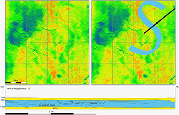
Fig. 6. Processed time slice from 3D seismics showing a buried ice-pushed ridge structure in the shallow subsurface of the Dogger Bank (upper panels). The subtle curved structure visible on a 3D seismic time slice, highlighted in light blue on the upper right panel, is correlated to glaciotectonically deformed units on a profile from high-frequency 2D seismics (bottom panel). This presumed Weichselian ice-pushed ridge from the Dogger Bank resembles structures of Saalian age preserved onland in the central Netherlands.
The relevance of these glacial landscapes from a perspective of human occupation is twofold. On the one hand, humans may have been present in the area during the glacial periods themselves, living in cold, continental conditions and profiting from tundras and periglacial floodplains during brief periods of interstadial conditions (cf. Pavlov et al., Reference Pavlov, Svendsen and Indrelid2001). Here, they would have found the conditions to hunt large herbivores. On the other hand, they will have used the morphology left behind by receding ice sheets to their advantage. During full interglacial circumstances, ridges would have been vantage points and lows would have provided freshwater sources, fish and game.
Reconstructed interglacial landscapes
The most complete reconstruction of interglacial palaeolandscapes was made for Doggerland (Gaffney et al., Reference Gaffney, Fitch and Smith2009, Reference Gaffney, Al Naimi, Cuttler and Fitch2011). Using 3D seismics, they found evidence of meandering rivers, mud flats, salt marshes, estuaries and lakes (Fig. 7). Others have recognised, inferred and mapped various nearshore landscape elements (Trentesaux et al., Reference Trentesaux, Stolk and Berné1999), deltas and river channels (Cameron et al., Reference Cameron, Stoker and Long1987; Salomonsen, Reference Salomonsen1993; Laban, Reference Laban1995; Hijma et al., Reference Hijma, Cohen, Roebroeks, Westerhoff and Busschers2012), river-margin inland-dune complexes (Fig. 4a; Hijma et al., Reference Hijma, Van der Spek and Van Heteren2010), coastal barriers (Rieu et al., Reference Rieu, Van Heteren, Van der Spek and De Boer2005), tidal inlets and tidal deltas (Kosters et al., Reference Kosters, Van Mierlo, Verbeek, Posthumus, McGee and Brouwer1992; Rieu et al., Reference Rieu, Van Heteren, Van der Spek and De Boer2005), tidal basins (Trentesaux et al., Reference Trentesaux, Stolk and Berné1999; Rieu et al., Reference Rieu, Van Heteren, Van der Spek and De Boer2005; Hijma et al., Reference Hijma, Van der Spek and Van Heteren2010), estuaries (Mathys, Reference Mathys2009) and freshwater marshes (Missiaen et al., Reference Missiaen, Murphy, Loncke and Henriet2002, from acoustic turbidity caused by shallow gas; Hijma et al., Reference Hijma, Cohen, Roebroeks, Westerhoff and Busschers2012, from cored and trawled organic deposits) of different ages, commonly from 2D data and on a limited lateral scale.
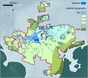
Fig. 7. Palaeolandscape reconstruction for part of the British and Dutch Continental Shelf on the basis of 3D seismics. Depositional features and relative topography were reconstructed.
Most of the identified landscape elements were formed and preserved during drowning phases governed by rapid relative sea-level rise at the end of the last glaciation. The 3D data analysed by Fitch et al. (Reference Fitch, Thomson and Gaffney2005) and Gaffney et al. (Reference Gaffney, Fitch and Smith2009) show how an upland area (Dogger Hills) was gradually transformed from a fluvially dominated area with a few lakes into a shrinking North Sea island (Dogger Island) fringed by tidal environments some 8500 years ago, which finally submerged and disappeared around 7000 years ago.
Some landscape elements with low preservation potential are merely inferred on the basis of evidence from related depositional environments. Rieu et al. (Reference Rieu, Van Heteren, Van der Spek and De Boer2005) reconstructed the presence and locations of a series of barrier islands from (i) the distribution of back-barrier tidal channels and (ii) the transition patterns in shell assemblages (back-barrier to mixed open-marine in a seaward direction; Fig. 8). It must be emphasised that the distribution of many palaeolandscape elements is unrelated to present-day bathymetry. Berné et al. (Reference Berné, Trentesaux, Stolk, Missiaen and De Batist1994), for example, showed that the core of offshore tidal ridges may consist of sediment deposited in tidal channels and deltas, and in estuaries during periods of lower relative sea level. The present shape of these ridges was shown to result from more recent erosion of the adjacent swales.

Fig. 8. Inference of the possible position of former barrier islands offshore from the western Netherlands using information on the positions and extents of tidal-channel fills as derived from high-frequency 2D seismics collected in a kilometre-sized grid (Rieu et al., Reference Rieu, Van Heteren, Van der Spek and De Boer2005).
The relevance of changing interglacial landscapes to human occupation can be viewed from both static and dynamic perspectives. From a static point of view, early humans will have preferred the most fertile and accessible areas, commonly near waterways and coastlines. From a dynamic point of view, they will have experienced river floods and storm surges, and learned to anticipate long-term climate- and landscape-related changes such as rising sea level (Leary, Reference Leary2009) and ecological succession.
Discussion
A need for validation
It could be tempting to reconstruct palaeolandscapes exclusively from seismic data, especially when these data are plentiful and other data types are not or only scantily available. When doing so, one must consider that the acoustic character of seismic facies is not always directly linked to sediment type (Stoker et al., Reference Stoker, Stewart, Paul and Long1992). Additionally, unaided (blind) interpretation of time slices is strongly driven by geomorphic analogy. Such an approach works well for common, easily recognisable landscape elements. However, it is possible to overlook poorly known or weakly expressed features. Thus, a validation of seismic data and its interpretations by a team of specialists with a broad range of expertise and knowledge of various sedimentary systems is essential. In the translation of 2D or 3D forms into landscape elements and from TWTT to depth, information from cores is indispensable. A fill of an imaged meandering channel, for example, may turn out to be either freshwater fluvial or saline tidal in character, and may show transitions between fluvial and tidal characteristics through time. Even the broader landscape context may not allow a full environmental interpretation. Unfortunately, cores providing information on more than the uppermost and shallowest sedimentary units are rare and widely spaced, especially in offshore areas with relatively great water depths far from the coast. Core samples on which environmental analyses (pollen, foraminifera, diatoms, ostracods, molluscs, geochemical and isotopic composition) and/or dating (14C or luminescence) have been performed are even rarer. Such analyses are essential for linking landscape elements of equal age and for the chronological ordering of landscape features. Even with these laboratory analyses available, the correlation of deeper landscape elements can be wrought with difficulty. In cross-correlating and determining the relative age of landscape elements, 2D seismics may be more suitable than 3D seismics, but data multiples and other such restrictions may still blur the picture (Fitch et al., Reference Fitch, Thomson and Gaffney2005). A combined approach using seismic data in conjunction with sufficient core material is required, and should therefore be an integral part of all future mapping surveys.
Models of landscape evolution
The identification of landscape elements is a major step in the reconstruction of palaeolandscapes and their associated topography. However, reconstructions also need to include non-preserved elements of the palaeolandscape, requiring a thorough knowledge of modern depositional environments and facies. When such reconstructions are made for large areas, the dynamic nature of the Earth’s surface is an additional complicating factor. It is the principal reason why preserved palaeosurfaces cannot be considered synonymous with palaeolandscapes, especially in the case of older (pre-glacial) surfaces. Dynamic models of landscape evolution need to consider buried surfaces and present-day bathymetry in light of their age, contemporary sea level (from regional studies of relative sea-level change, including assessments of glacio-isostatic adjustment), and past sediment sources and sinks (Gaffney et al., Reference Gaffney, Fitch and Smith2009; Sturt et al., Reference Sturt, Garrow and Bradley2013).
Correction of palaeosurfaces for crustal motion is particularly important for understanding the speed and mode of transition from terrestrial periglacial to marine environments at the end of the last Ice Age, from the final millennia of the Last Glacial Maximum to the early Holocene (16,000–8000 years ago). When glacio-isostasy and the degree to which middle- and late-Holocene coastal and marine processes (i.e. during the past 8000 years) have eroded drowned palaeosurfaces can be quantified, it may become feasible to establish and finetune the timing of transgressions, to reconstruct changing coastline positions and to constrain rates of inundation. Following corrections, including those for sedimentation, particularly when the bathymetry is used as a palaeolandscape indicator (Fig. 9), it may become possible to demonstrate land loss over time at high temporal resolution for inundated areas such as Doggerland and various smaller (former) islands, and to understand the implication of change for past societies. For the various lowstand phases, an important issue is the recognition and timing of changes in river drainage (Hijma et al., Reference Hijma, Cohen, Roebroeks, Westerhoff and Busschers2012). These changes may shed light on associated climate and environmental change. Identification of Pleistocene landscape elements associated with proglacial lakes and scoured spillway channels is an additional gap in our current knowledge that may also be filled using high-density or 3D seismic data.
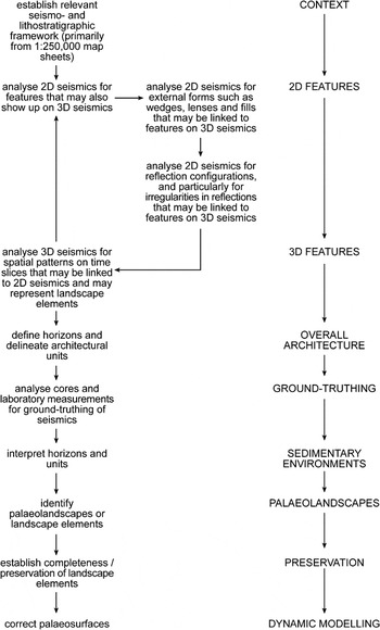
Fig. 9. Required steps to proceed from 2D and 3D seismics to palaeolandscape models.
Marine truncation of palaeosurfaces can be easily recognised on high-frequency 2D seismics (e.g. Berné et al., Reference Berné, Trentesaux, Stolk, Missiaen and De Batist1994; Rieu et al., Reference Rieu, Van Heteren, Van der Spek and De Boer2005). When combined with lithostratigraphic data, good regional coverage of seismic data provides insight into the degree of intactness of palaeolandscapes. Of all landscape elements, palaeovalleys have the highest significant chance of being preserved and identified. Their fills provide caches of environmental data that can be used to understand past landscape changes (Gaffney et al., Reference Gaffney, Fitch and Smith2009). Areas in which palaeosurfaces are no longer intact may still provide valuable information on past landscapes. Lag deposits, such as ravinement surfaces caused by wave-driven truncation of drowning landscapes, tend to concentrate faunal remains (cf. Hijma et al., Reference Hijma, Cohen, Roebroeks, Westerhoff and Busschers2012) and probably also human artefacts. Awareness of reworking helps to put these finds into their correct geological context, including the number of reworking events or the final reworking event. In addition, archaeologically relevant material in lag deposits may provide insight into periods that have not been sampled in an undisturbed context. Within the North Sea, the degree of reworking increases from north to south, with the Quaternary sequence becoming increasingly thin. The few surficial ravinement lags in the north contain only Last Glacial and Holocene material, whereas those in the south include even Pliocene material.
The generation of comprehensive palaeolandscape models for different warm and cold phases in the Quaternary of the North Sea increasingly appears to be achievable, although many challenges still remain. Data gaps must be filled, both spatially and temporally, with particular emphasis on preserved landscape elements from before the last glaciation. Additionally, there is a need for increased, and optimised, data integration across national borders. When supplemented with 2D seismics, core logs and laboratory analyses, 3D seismic data provide the potential to spawn a new generation of maximum-coverage palaeolandscape and archaeological potential (or suitability) models, not only because of their spatial coverage, but also because of the opportunities they offer to optimise future strategies for the collection of new core and geophysical data (Fitch et al., Reference Fitch, Thomson and Gaffney2005).
Acknowledgements
This paper is a contribution to COST Action TD0902 SPLASHCOS (Submerged Prehistoric Archaeology and Landscapes of the Continental Shelf), supported by the European Science Foundation and the European Union Research Training and Development Framework Programme. Peter Roll Jakobsen and Jörgen Leth (GEUS) provided a new, unpublished version of the geomorphological map of Denmark (incorporated in Fig. 5). Guest editor Kim Cohen and two anonymous reviewers provided useful comments on the original manuscript.


