


1. INTRODUCTION
Frontal ablation, that is, ice mass losses by calving, subaerial frontal melting and sublimation and subaqueous frontal melting (Cogley and others, Reference Cogley2011), is an important component of the mass balance of tidewater glaciers and marine-terminating ice caps. It has been reported to account for up to 30–40% of the total ablation of some Arctic glacierised archipelagos and ice caps (Dowdeswell and others, Reference Dowdeswell2002, Reference Dowdeswell, Benham, Strozzi and Hagen2008; Błaszczyk and others, Reference Błaszczyk, Jania and Hagen2009) and up to 50% in some ice caps in the Antarctic periphery (Osmanoğlu and others, Reference Osmanoğlu, Navarro, Hock, Braun and Corcuera2014). Because of the difficulty of calculating the components of frontal ablation separately, it is usually approximated by the ice discharge through flux gates close to the calving fronts, calculated as the product of ice velocity and cross-sectional area (volumetric flux). If the considered flux gate is not close to the calving front, the surface mass balance between them should be taken into account (Andersen and others, Reference Andersen2015; McNabb and others, Reference McNabb, Hock and Huss2015). Neglecting this effect will in nearly all cases lead to an overestimation of the frontal ablation. For Alaskan glaciers, McNabb and others (Reference McNabb, Hock and Huss2015) found an overestimate of 19% on average for individual glaciers (10% for the regional total). For Canadian Arctic glaciers the overestimate is expected to be larger, because of the strongly negative recent surface mass balance of this region (Gardner and others, Reference Gardner2011). Possible front position changes should also be taken into consideration (Burgess and Sharp, Reference Burgess and Sharp2004; Burgess and others, Reference Burgess, Sharp, Mair, Dowdeswell and Benham2005; Williamson and others, Reference Williamson, Sharp, Dowdeswell and Benham2008; Van Wychen and others, Reference Van Wychen2016), though the terminus advance/retreat is in general expected to account for a smaller share of the frontal ablation estimates. For instance, McNabb and others (Reference McNabb, Hock and Huss2015) indicated an overestimation of 13% (2% of the regional total) by neglecting advance/retreat of the terminus for Alaskan glaciers. This effect is more difficult to quantify for the Canadian Arctic glaciers due to the pulsating behaviour of many of them (Williamson and others, Reference Williamson, Sharp, Dowdeswell and Benham2008; Van Wychen and others, Reference Van Wychen2016, Reference Van Wychen2017). Pulsating glaciers, as surging glaciers, show periods of speedup and slowdown. However, the velocity variability of pulsating glaciers is restricted to their lowermost terminal zone, which is grounded below sea level. Additional factors influencing frontal ablation estimates, such as cross-sectional ice-thickness variations and long-term thickness changes have been discussed, e.g. by McNabb and others (Reference McNabb, Hock and Huss2015). The seasonality of the glacier velocity measurements can also have a noticeable impact on frontal ablation estimates, with seasonal velocity amplitudes averaging ~50% of the peak velocity for Alaskan glaciers (McNabb and others, Reference McNabb, Hock and Huss2015) and ~45% in Livingston Island, off the northwestern Antarctic Peninsula (Osmanoğlu and others, Reference Osmanoğlu, Navarro, Hock, Braun and Corcuera2014). The changes for the Canadian Arctic glaciers seem to be more modest, with a seasonal variability of ~10–20% of the average values (Van Wychen and others, Reference Van Wychen2012). The interannual variations of glacier velocity are also an important issue, particularly for the Canadian Arctic glaciers due to their pulsating nature. Estimates of total error in frontal ablation accounting for the various error sources described above are typically within ~20–30%. For instance, values of 24 and 25% have been given for some Alaskan glaciers by McNabb and others (Reference McNabb, Hock and Huss2015) and Vijay and Braun (Reference Vijay and Braun2017), respectively, while a value of 31% has been given by Van Wychen and others (Reference Van Wychen2016) for the Canadian High Arctic.
In this paper, we will focus on analysing the errors in the ice discharge estimates through given flux gates, so we will refer to ice discharge rather than frontal ablation. A fundamental problem for estimating the ice discharge is that very often the cross-sectional area of tidewater glaciers is unknown. Normally, there is a lack of information regarding the thickness of glaciers. Typically, glacier thickness is only known along the central flowline, sometimes on the glacier's cross section and very rarely both of them are available for a specific glacier (Leuschen and others, Reference Leuschen, Gogineni, Rodriguez-Morales, Paden and Allen2010). This scarcity in ice-thickness data motivates the use of U-shaped cross-sectional profiles for ice discharge estimates when only ice-thickness data along the glacier flowline is available (Van Wychen and others, Reference Van Wychen2012). Inverse modelling is used when we count on little ice-thickness data, or no data at all (Farinotti and others, Reference Farinotti, Huss, Bauder, Funk and Truffer2009). Observed thickness data can be assimilated into inverse methods (Osmanoğlu and others, Reference Osmanoğlu, Braun, Hock and Navarro2013, Reference Osmanoğlu, Navarro, Hock, Braun and Corcuera2014).
Different approaches have been taken in the literature to estimate the error in ice discharge through flux gates. However, most of them only provide upper and lower bounds of the error (Burgess and others, Reference Burgess, Sharp, Mair, Dowdeswell and Benham2005; Van Wychen and others, Reference Van Wychen2012), rather than statistical estimates of the expected error with a certain degree of uncertainty. In this paper, we aim to contribute to fill this gap by analysing, using error propagation, the various error sources involved in the estimate of ice discharge, and to quantify their individual contributions to the total error in ice discharge.
When cross-sectional ice-thickness measurements are not available, ice-discharge estimates through given flux gates can be based on an increasingly complex approach, ranging from the so-called box-shaped approaches (Brown and others, Reference Brown, Meier and Post1982; Rignot and others, Reference Rignot, Box, Burgess and Hanna2008; Williamson and others, Reference Williamson, Sharp, Dowdeswell and Benham2008; Błaszczyk and others, Reference Błaszczyk, Jania and Hagen2009; Burgess and others, Reference Burgess, Forster and Larsen2013) to those considering a varying cross-sectional depth (Van Wychen and others, Reference Van Wychen2012, Reference Van Wychen2014, Reference Van Wychen2015, Reference Van Wychen2016, Reference Van Wychen2017). The box-shaped approach shows a tendency to overestimate the ice discharge, so we will not use it in this paper. Various U-shaped approaches can be taken, and a detailed analysis of their performance, on the basis of the comparison of their results with those for a large set of observed cross-sectional areas, is lacking in the literature. Filling this gap is the second aim of the present paper.
The two above analyses will be based on ice discharge estimates for the Canadian High Arctic using ice-thickness data and remotely sensed glacier surface-velocity data from 2012–15 and 2016/17 respectively. This will provide, as a by-product of this paper, updated ice-discharge estimates for glaciers of the Canadian High Arctic during 2016/2017.
2. STUDY SITE AND DATA
The Queen Elizabeth Islands (Ellesmere, Axel Heiberg and Devon islands) are located in the Canadian Arctic, neighbouring the western coast of Greenland (Fig. 1a). This region is often referred to as Canadian High Arctic. The ice masses of Ellesmere Island contain one-third of the global volume of land ice outside Greenland and Antarctica (Radić and Hock, Reference Radić and Hock2010) with a glacierised area in 2000 of ca. 104 000 km2 (Sharp and others, Reference Sharp, Kargel, Leonard, Bishop, Kääb and Raup2014) while Devon Ice Cap covers ~ 14 000 km2 and is one of the largest ice caps in the Arctic (Dowdeswell and others, Reference Dowdeswell, Benham, Gorman, Burgess and Sharp2004). The dynamics of Canadian Arctic glaciers and ice caps have been extensively studied (Copland and others, Reference Copland, Sharp and Dowdeswell2003; Dowdeswell and others, Reference Dowdeswell, Benham, Gorman, Burgess and Sharp2004; Burgess and others, Reference Burgess, Sharp, Mair, Dowdeswell and Benham2005; Williamson and others, Reference Williamson, Sharp, Dowdeswell and Benham2008; Gardner and others, Reference Gardner2011; Van Wychen and others, Reference Van Wychen2012, Reference Van Wychen2014, Reference Van Wychen2015, Reference Van Wychen2016; Millan and others, Reference Millan, Mouginot and Rignot2017; Strozzi and others, Reference Strozzi, Paul, Wiesmann, Schellenberger and Kääb2017). Copland and others (Reference Copland, Sharp and Dowdeswell2003) made an analysis on the surge-type glaciers in this region and later studies by Van Wychen and others (Reference Van Wychen2016, Reference Van Wychen2017) developed a classification scheme into three glacier types depending on their dynamics: surging, pulsing and consistent acceleration/deceleration. These investigations indicate that the glaciers of the Canadian High Arctic show marked differences in dynamic behaviour, and large spatial and temporal variabilities.
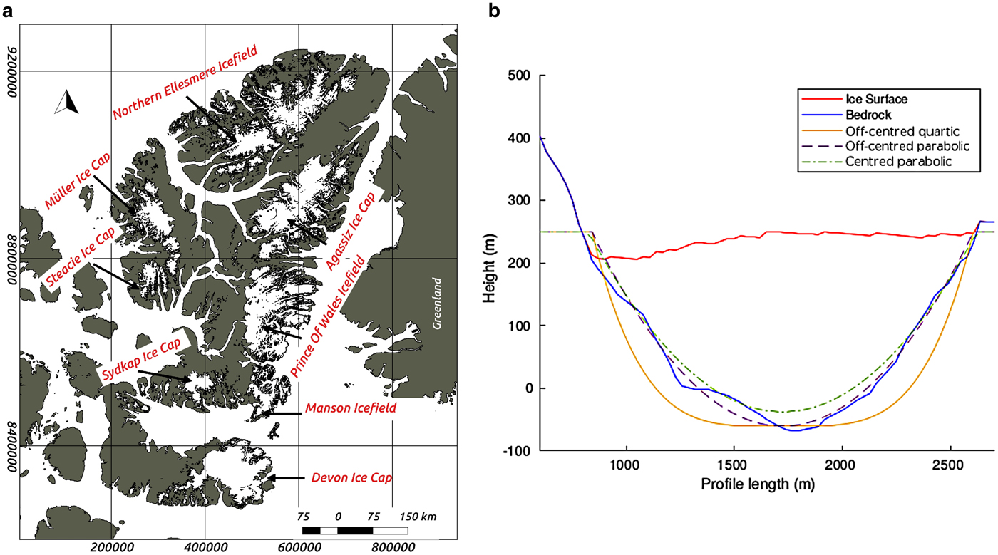
Fig. 1. (a) Main ice masses of Ellesmere, Axel Heiberg and Devon Islands, Canadian High Arctic (Wessel and Smith, Reference Wessel and Smith1996). The glacier outlines are from the Randolph Glacier Inventory (RGI) version 5.0 (Pfeffer and others, Reference Pfeffer2014). See more detail in Supplementary Materials figures S1, S2 and S3, and Table S1. (b) Cross-sectional profile approaches overlaid on a real glacier cross section. All maps in this paper use the Universal Transverse Mercator (UTM) projection of the zone 17 north, and the reference ellipsoid is WGS84.
The datasets used in this study encompass synthetic aperture radar (SAR) images from the Sentinel-1 platform, Operation IceBridge airborne radar ice thickness (Leuschen and others, Reference Leuschen, Gogineni, Rodriguez-Morales, Paden and Allen2010; Gogineni, Reference Gogineni2012) and the freely accessible Canadian DEM (CDEM) designed by Natural Resources Canada (NRCan) with a resolution of 0.75 and 3 arcsec in the southnorth and westeast directions, respectively (NRCAN, 2016). The DEM was used for geocoding and co-registering the imagery employed for the intensity offset tracking technique. ArcticDEM from WorldView satellite, from 2012 and 2014–15, was used for estimating local ice-thickness changes from surface-elevation changes, assuming no glacier-bed elevation change.
The surface velocities on the Canadian High Arctic were obtained from SAR Terrain Observation by Progressive Scans (TOPS) Interferometric Wide (IW) Level-1 Single Look Complex (SLC) images. These products provide a geo-referenced image (using accurate altitude and orbital information from the satellite), in slant-range geometry, processed in zero-Doppler (Geudtner and others, Reference Geudtner, Torres, Snoeij, Davidson and Rommen2014). The image is normally composed of three sub-swaths with each sub-swath comprising normally nine consecutive bursts, which overlap in azimuth. Burst synchronisation is needed for interferometry and for accurate offset tracking (Holzner and Bamler, Reference Holzner and Bamler2002). The resolution of Sentinel-1 SAR TOPS IW mode is of 5 and 20 m in the range and azimuth directions, respectively. The SAR images used in this study were acquired during the winter of the year 2016 (beginning of February until mid-March) and the winter of the following year (end of January to mid-March 2017). See more detail in Supplementary Materials Table S2.
The ice-thickness dataset lumps a wide variety of data regarding both acquisition dates and geographical distribution (Table 1). In particular, we count on transverse ice-thickness profiles for 23 glaciers, and 20 additional glaciers for which only along-flow, close to centreline ice-thickness profiles are available, totalling 43 studied glaciers in the area. Ice-thickness data were measured using the Multichannel Coherent RADAR Depth Sounder (MCoRDS) (Leuschen and others, Reference Leuschen, Gogineni, Rodriguez-Morales, Paden and Allen2010). Specifically, the dataset used in this study is the post-processed L2, which contains information about time, latitude, longitude, elevation, glacier surface and bed elevation, and ice thickness, the latter one with an estimated uncertainty of ±10 m (Gogineni, Reference Gogineni2012).
Table 1. Operation IceBridge airborne radar profiles used in this study. Cross means cross-sectional profiles and Long means longitudinal (along-flow, close to glacier centreline) profiles

3. METHODOLOGY
We calculate the ice discharge using a flux-gate approach for two cases: (1) the cross-sectional depth profile is known (Vijay and Braun, Reference Vijay and Braun2017), and (2) the cross section is estimated using an approximation to the depth profile (Harbor, Reference Harbor1992; Cuffey and Paterson, Reference Cuffey and Paterson2010). For the latter case, we will use three different approaches, a centred parabola for which the ice thickness at the glacier centreline is assumed to be known, a centred parabola with ice thickness known at an off-centred point and a quartic function with ice thickness known at an off-centred point. The availability of airborne radar cross-sectional profiles for 23 Canadian High Arctic glaciers, which will be taken as reference, will allow us to compare the accuracy of the various cross-sectional area approaches.
3.1. Ice discharge
Ice discharge is calculated as mass flux per unit time across a given surface S approximated per area bins as
 $$\phi=\int_{S} \rho {\bf v} \cdot {\bf dS} = \sum_{i}{\rho L_i H_i f v_i \cos \alpha_i},$$
where ρ is ice density, L i and H i are respectively the width and thickness of an area bin, f is the ratio of surface to depth-averaged velocity, f ∈[0.8,1] (Thomas and others, Reference Thomas2000; Cuffey and Paterson, Reference Cuffey and Paterson2010; Andersen and others, Reference Andersen2015), v i is the magnitude of surface velocity and α i is the angle between the surface velocity vector and the direction normal to the local flux-gate for the bin under consideration. When airborne radar cross-sectional profiles are available, we define the bin widths and orientations as given between consecutive radar-measured points; when no cross-sectional airborne radar profiles are available, we use bins of fixed width and thickness estimated from the corresponding cross-sectional profile approach, and the velocity vector orientations are calculated with respect to the vector normal to the cross section.
The above-described approach for the calculation of ice discharge is valid for grounded sections of tidewater glaciers. The analysis of the available radar profiles, together with the flotation criterion, indicates that a few of the studied glaciers have floating tongues or are close to flotation, in agreement with Williamson and others (Reference Williamson, Sharp, Dowdeswell and Benham2008). However, in all cases we have calculated the fluxes at locations where the glaciers are grounded.
3.2. Cross-sectional profile approaches
When airborne radar data are only available along a profile close to the glacier central flowline, the set of points to be used for approximating the cross-sectional thickness profile is limited to three points: the intersection of the longitudinal radar profile with the selected cross section and the intersection of the cross section with the glacier margins. In the two latter points, zero ice thickness is most often assumed.
We consider in our analysis three different approaches to the cross-sectional area of a tidewater glacier (Fig. 1b). The first approach is the one used by Van Wychen and others (Reference Van Wychen2014, Reference Van Wychen2016), who used a parabola with axis at the glacier centreline, assuming that the radar-measured ice thickness H m corresponds to the glacier centreline (Fig. 2 with H m = H c) and that the ice thickness at both margins, x = ±W, is of 10 m; for short, we will refer to this approach as centred parabolic. The ice thickness H at a point situated at a distance x from the glacier centreline is then given by
 $$ H(x)= {10-H_{\rm m} \over W^{2}} x^{2} + H_{\rm m},$$
where we have renamed the variables and parameters used by Van Wychen and others (Reference Van Wychen2014, Reference Van Wychen2016) as follows: H m = C, W = D 1 and x = D 2.
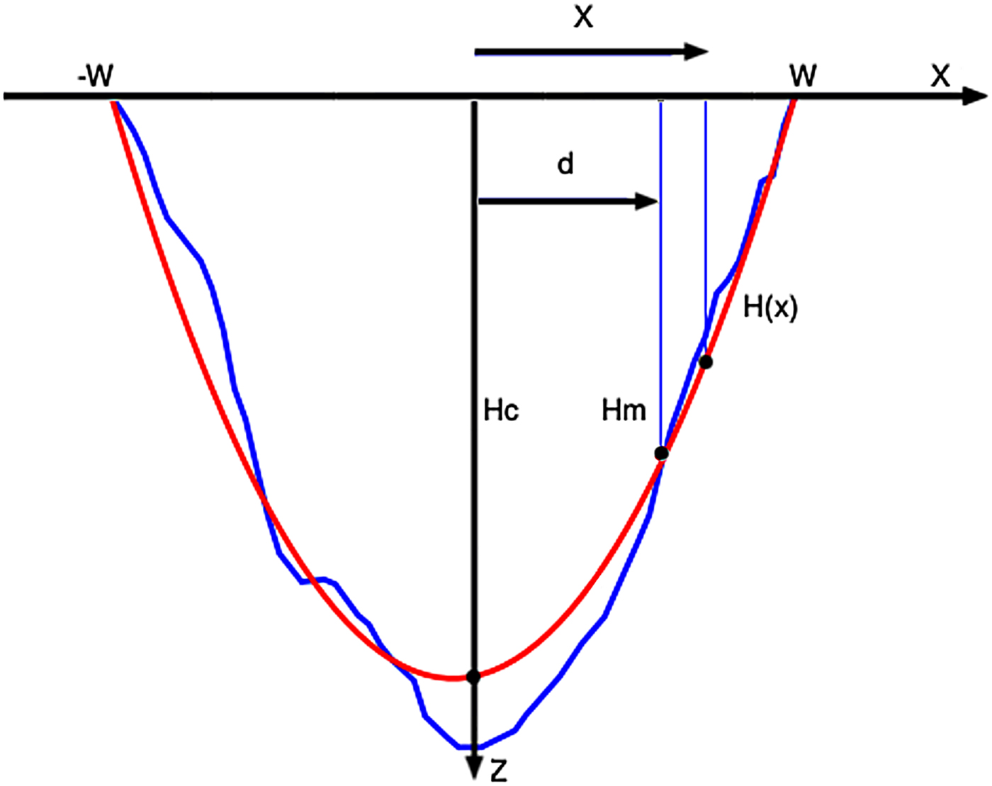
Fig. 2. Geometry of the U-shaped cross-sectional approaches used in this study. The blue line represents the actual cross profile of Glacier North 3 (Fig. S3) from NASA Operation Ice-Bridge data acquired 4 May 2012, while the red line represents its U-shaped approximation. H m is the radar-measured ice thickness and H c is the ice thickness at the glacier centreline. W is the glacier half-width.
The second approach, also of parabolic type and with axis located at the glacier centreline, differs in that H m is not assigned to the centreline but is located at a distance d from it (Fig. 2). This is more realistic as it represents the possibility that the radar longitudinal profile could have an offset from the glacier centreline. In this case, we have assumed zero ice thickness at the margins. For short, we will refer to this approach as off-centred parabolic. The equation considered is of the type
 $$H(x) = a x^{2} + b,$$
which, upon applying the constrain that the parabola passes through the points (W, 0) (or ( − W, 0)) and (d, H), where W represents the glacier half-width, becomes
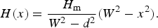 $$H(x) = {H_{\rm m} \over W^{2}-d^{2}} (W^{2} - x^{2}).$$
When d=0, i.e. the radar flight line coincides with the glacier centreline, the latter equation reduces to Eqn (2), except for the addend 10.
The third approach is similar to this second one except that the function is now a quartic polynomial of the type
 $$H(x) = a x^{4} + b,$$
which, again, upon the constraint of passing through the points (W, 0) and (d, H), becomes
 $$H(x) = {H_{\rm m} \over W^{4}-d^{4}} (W^{4} - x^{4}).$$
For short, we will refer to this approach as off-centred quartic.
3.3. Intensity offset-tracking velocities
We applied SAR offset tracking algorithm in GAMMA Remote Sensing software in order to produce ice-surface velocity fields in range and azimuth directions from Sentinel-1 TOPS IW SLC Level-1 image pairs (Wegmüller and others, Reference Wegmüller2016). The particularity of the procedure lies in the use of range offsets from ascending and descending passes, avoiding the use of azimuth offsets, since Sentinel-1 data show a lower resolution in the azimuth direction. Simultaneously, we avoid the undesired ionospheric effect manifested in the data as azimuth streaks (Sánchez-Gámez and Navarro, Reference Sánchez-Gámez and Navarro2017). We performed the error analysis for Ellesmere Island, focusing on the performance of the algorithm on stable ground (on ice-free areas on the western side of Prince of Wales Icefield). The area under consideration was ~150 km2, involving ~4700 velocity samples. The use of this novel approach allowed us to obtain an improved velocity field with a RMSE of 0.012 m d−1. Nevertheless, we decided to take a conservative error estimate of 0.021 m d−1 for the surface velocity field, resulting from one 20th of the range direction resolution as suggested by Strozzi and others (Reference Strozzi, Luckman, Murray, Wegmuller and Werner2002) and Werner and others (Reference Werner, Wegmüller, Strozzi and Wiesmann2005).
We used a matching window of 320 pixel × 64 pixel (1200 m × 1280 m) in the range and azimuth directions, respectively, with an oversampling factor of 2 for improving the tracking results. The sampling steps were of 40 pixel × 8 pixel and the resolution of the final velocity map was 200 m × 160 m in the range and azimuth directions. The geocoding was completed using the CDEM. We used a bicubic spline interpolation to generate the geocoded grid. The determined velocities fields were manually checked for mismatches in all glacierised areas. These artefacts were removed from the dataset. We paid special attention to those areas where ice discharge was calculated.
3.4. Error analysis
Two types of error estimates for ice discharge are considered in the literature. The first one uses upper and lower bounds for the input values (i.e., velocity and thickness), resulting in upper and lower bounds for the ice flux (Burgess and others, Reference Burgess, Sharp, Mair, Dowdeswell and Benham2005; Williamson and others, Reference Williamson, Sharp, Dowdeswell and Benham2008; Van Wychen and others, Reference Van Wychen2012). The second approach consists of estimating the statistically expected error using error propagation from the individual error components (Andersen and others, Reference Andersen2015; Vijay and Braun, Reference Vijay and Braun2017; Gardner and others, Reference Gardner2018), and requires that all the considered errors are independent and uncorrelated. In our analysis, we follow the latter approach.
3.4.1. Case 1: cross-sectional profiles of ice thickness are available
Applying error propagation to Eqn (1) we get
 $$\sigma_{\phi} = \sqrt{\sigma_{\phi_{\rho}}^{2}+\sigma_{\phi_f}^{2}+\sigma_{\phi_H}^{2}+\sigma_{\phi_v}^{2}+\sigma_{\phi_{\alpha}}^{2}},$$
where the various terms represent the contribution to the error in ice discharge due to the uncertainties in density ( $\sigma_{\phi_\rho }$), ratio of surface to depth-averaged velocity (
 $\sigma_{\phi_f}$), ice thickness (
 $\sigma_{\phi_H}$), velocity modulus (
 $\sigma_{\phi_v}$) and direction (
 $\sigma_{\phi_\alpha }$), and each of the terms is of the form (taking
  $\sigma_{\phi_H}$ as an example)
 $$\sigma_{\phi_H} = \sqrt{\sum_{i}{(\sigma_H \rho L_i f v_i \cos \alpha_i)}^{2}}.$$
 In Eqn (7), we have omitted a term  $\sigma_{\phi_L}^{2}$ because the bin width L i is assumed to be error-free. As error estimates for the ice thickness and surface velocity we took σ H = 10 m (Gogineni, Reference Gogineni2012) and σ v = 0.021 m d−1 (Strozzi and others, Reference Strozzi, Luckman, Murray, Wegmuller and Werner2002; Sánchez-Gámez and Navarro, Reference Sánchez-Gámez and Navarro2017). Regarding the ratio of surface to depth-averaged velocity (f), it is considered in the literature that f ∈[0.8,1] (Cuffey and Paterson, Reference Cuffey and Paterson2010). To give a good approximation for this parameter an analysis of the driving stresses present in a glacier and its derived flow regimes would be advisable (Dowdeswell and others, Reference Dowdeswell, Benham, Gorman, Burgess and Sharp2004; Burgess and others, Reference Burgess, Sharp, Mair, Dowdeswell and Benham2005; Van Wychen and others, Reference Van Wychen2017). However, simple observation of the glacier surface features could give a hint on the flow regime and therefore help to better constrain f. Normally, tidewater glacier velocity at the terminus is dominated by basal sliding which makes f close to unity. Van Wychen and others (Reference Van Wychen2016), who used the error-bound approach, assumed lower and upper bounds for f of 0.8 and 1, respectively, while Andersen and others (Reference Andersen2015) and Vijay and Braun (Reference Vijay and Braun2017), who used the statistical-error approach, took f = 0.93 ± 0.05. We have also taken the latter value and error estimate for f. For ice density, we took ρ = 900 ± 17 kg m−3. Finally, for calculating σ α we used a moving window encompassing 10 velocity measurements along the cross section and calculated the standard deviation (std dev.) of their orientations with respect to the normal to the cross section.
The error in ice discharge given by Eqn (7) assumes that the radar ice-thickness measurement and the velocity data are temporally coincident. This assumption is often not true. In particular, in our case study, both data acquisitions are separated by 1–5 years, depending on the glacier, and the glaciers can be expected to have undergone an ice-thickness change during that period. We take this into account by calculating the thinning (or thickening) rate and estimating the change in flux implied by the assumption of simultaneity of airborne radar and SAR acquisitions. This amount constitutes a systematic error (a bias), which we will represent as  $\epsilon_{\phi_{{(\partial h}/{\partial t})}}$ and that should be accounted for in our discharge calculations. This factor should not be disregarded, as Van Wychen and others (Reference Van Wychen2016) have pointed out substantial thinning rates in this region during 1999–2015. These rates are highly variable depending on each particular glacier, and are important even when considering short periods of time because of the pulsating behaviour of many of these glaciers (Van Wychen and others, Reference Van Wychen2016, Reference Van Wychen2017). The surface elevation change of a tidewater glacier does not always indicate ice-thickness change, especially near the glacier fronts where flotation can occur. As discussed earlier, some of the studied glaciers have floating tongues or are close to flotation. However, in all cases, we have calculated the fluxes at locations where the glaciers are grounded, so we can safely assume that surface elevation changes correspond to ice thickness changes.
We calculated the thinning rates as difference in surface elevation between the radar data points (Icebridge data collected within 2012–15, depending on the glacier) and the corresponding points in a suitable DEM, for which we used the ArcticDEM from WorldView satellite, available for 2012 and 2014/15. To make the computation interval of the thinning rate long enough, we used the pairs radar 2012 with DEM 2014–2015, and radar 2014/15 with DEM 2012. The thinning rates were afterwards multiplied by the time interval between radar and SAR acquisitions to obtain the  $\epsilon_{\phi_{{(\partial h}/{\partial t})}}$ correction.
But, in addition to this systematic correction, the random nature of the thickness change (some glaciers thin while others thicken, the thinning rates change with time) requires to consider an error in thickness more conservative than that given by  $\sigma_{\phi_H}$. We do this by introducing an error
  $\sigma_{\phi_A}$, calculated as an error bound for the cross-sectional area due to the uncertainty in ice thickness. We compute the magnitude of this error as the area of a band of 10-m thickness (the value of σ H) all along the glacier cross section. The cross-sectional area incremented (decremented) by the area of this band will give us the upper (lower) bound for the cross-sectional area. If Eqn (7) is used with
  $\sigma_{\phi_H}$, we will denote the total error in flux as σ ϕ(H−based); if, instead, it is calculated using
  $\sigma_{\phi_A}$, then the total error in flux will be represented as σ ϕ(A−based). Obviously, σ ϕ(A−based) > σ ϕ(H−based), so σ ϕ(A−based) provides a more conservative approach to the estimate of the discharge error. The use of σ ϕ(H−based) is only recommended in cases where the radar and SAR acquisitions are simultaneous or very close in time; otherwise, the use of σ ϕ(A−based) is recommended.
3.4.2. Case 2: only centreline profiles of ice thickness are available
When only radar profiles along the glacier centreline are available, we are forced to make an assumption on the cross-sectional area, and its associated uncertainty will become the dominant error source in the discharge calculation. We will estimate the error in cross-sectional area by comparing, for the 23 glaciers for which a radar cross profile is available (see Table 2), the areas calculated for the known cross section with those estimated using each of the three U-shape approaches described in Section 3.2. These approaches are based on an interpolation through the points of measured ice thickness and the intersection of the cross section with the glacier margins. Since the flight lines do not follow exactly the glacier centreline, we are interested in determining the error in cross-sectional area as a function of the distance d between the glacier centreline and the radar flight line. With this aim, and to be able to compute some statistics on the errors, the areas and lengths of the cross sections of all 23 glaciers are normalised to unity, and each glacier's half-width is divided into 30 bins of equal length. Then, for each of the U-shape approaches and for each of the glaciers, a cross profile is calculated passing through each measured radar data point plus the two points at the glacier margins (Fig. 2), and the areas of the resulting U-shape profiles are calculated. Their differences with the corresponding known cross-sectional areas are taken as errors in cross-sectional area. Then, for each of the 30 bins, we compute the mean and the std dev. of the errors in cross-sectional area calculated for all the radar data points in the bin and for all 23 glaciers. The calculated mean represents the bias of the estimated cross-sectional area, and the calculated standard error (SE) will be taken as an error estimate of the cross-sectional area for the distance d under consideration (distance from the central point of the bin to the glacier centreline). Thus, the described procedure provides a bias and an error estimate for the cross-sectional area as a function of the distance d between the radar flight line and the glacier centreline, as shown in Figure 3 (we assume that the errors are equal at corresponding distances at each side of the centreline).
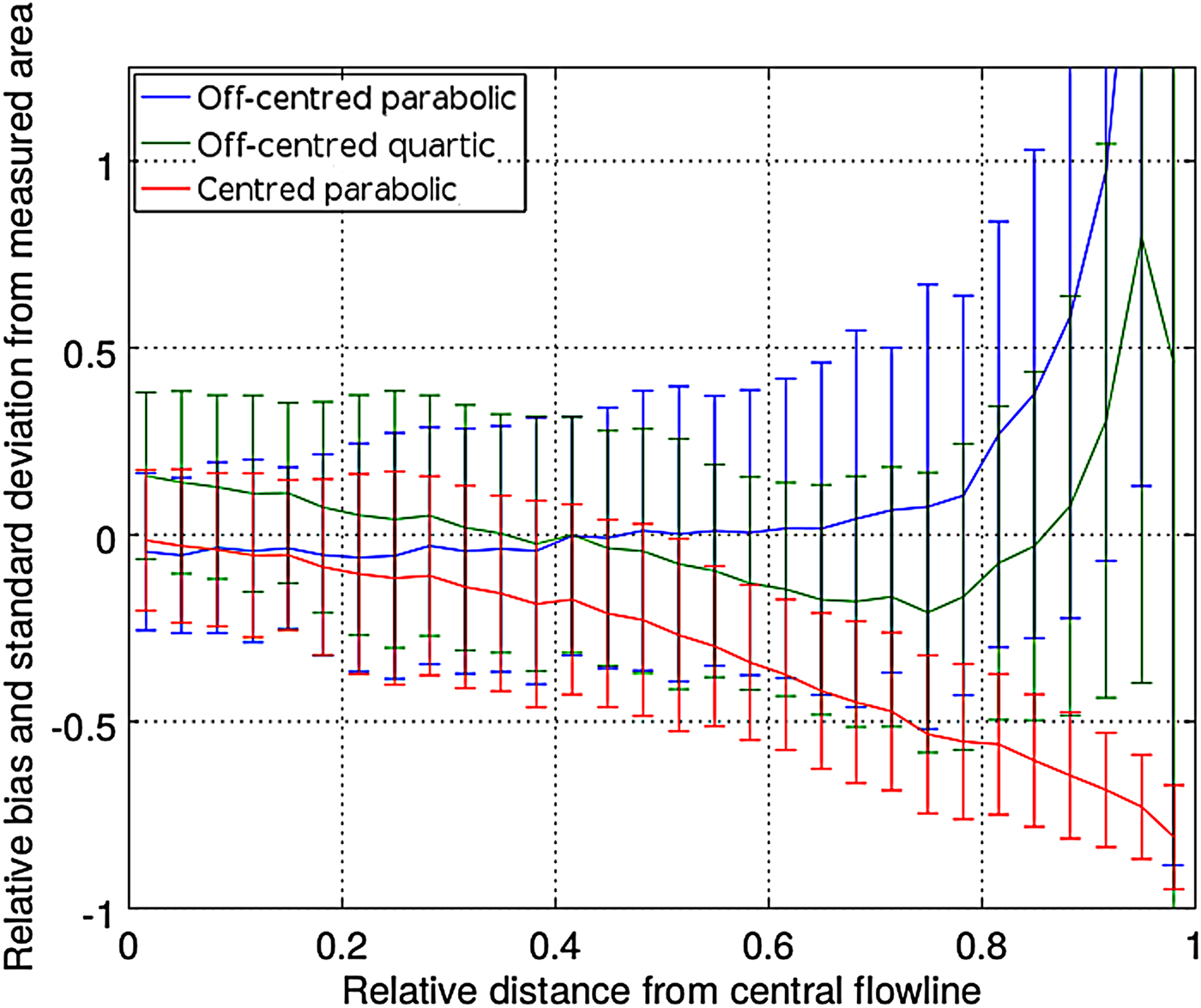
Fig. 3. Normalised cross-sectional area errors for the three different U-shape approaches, as a function of the normalised distance between the radar flight line and the glacier centreline. The vertical bars represent the std dev., and the distance from the centre of each bar to the zero line represents the corresponding bias. The continuous lines indicate the variation of the bias with the normalised distance. The blue bars/lines correspond to the off-centred parabolic approach, the green ones to the off-centred quartic approach, and the red ones to the centred parabolic approach of Van Wychen and others (Reference Van Wychen2014).
Table 2. Ice discharge using observed radar cross-sectional profiles
4. RESULTS AND DISCUSSION
4.1. Computed ice discharge and estimated errors for glaciers with radar cross-sectional profiles
Table 2 shows the discharge results obtained, for the winters of 2016 and 2017, for all glaciers with available cross-sectional radar profiles, together with their corresponding error estimates and the detail of the various error components. The discharge values are given in Mt a−1, and thus correspond to the extrapolation of winter estimates (typically, end of January to mid-March) to annual values. The annual values should not differ much from those given here, as the end-of-winter glacier velocities in the Canadian High Arctic are very close to their annual averages (e.g. 13.6% lower for Ellesmere and Axel Heiberg glaciers (Van Wychen and others, Reference Van Wychen2016)), and the seasonal variability is typically not large (e.g. within 10–20% for Devon glaciers (Van Wychen and others, Reference Van Wychen2012)). Moreover, the discharge values given by e.g. Van Wychen and others (Reference Van Wychen2016) and Millan and others (Reference Millan, Mouginot and Rignot2017) also correspond to approximately the same period in the year, which makes the comparison of results simpler.
We note that the estimated error in discharge due to the errors in the angle between the velocity vector and the vector normal to the cross section,  $\sigma_{\phi_{\alpha }}$, was negligible as compared with the rest of error components and therefore it has been excluded from the table. Discharge values for North 1 and Ekblaw Glaciers in 2016 are not given because of unavailability of proper SAR data.
As described in the ‘Methods’ section, we give two different estimates of the total error in ice discharge: σ ϕ(H−based), to be used in the case of temporarily coincident radar measurements and SAR acquisitions, and a more conservative error estimate σ ϕ(A−based), to be used otherwise. For some glaciers, this distinction does not imply a significant difference in the error estimates. However, in other cases σ ϕ(A−based) is up to three to five times larger than σ ϕ(H−based), as happens for the largest glaciers (Wykeham and Trinity). It is also three times larger for some medium-size glaciers (Fitzroy, South Crocker, Eastern) and three to five times larger for some small-size glaciers (East, Leffert). On average, σ ϕ(H−based) is 5% of the discharge and σ ϕ(A−based) is 8%, though individual values can be as high as 21% (South Margin) to 25% (Stygge) for σ ϕ(H−based), and 23% (South Margin) to 26% (Stygge) for σ ϕ(A−based).
The percentage values given under column  $\epsilon_{\phi_{({\partial h}/{\partial t}})}$ represent the change in discharge implied by the consideration of glacier thinning (negative values) or thickening (positive values) between the radar and SAR data acquisitions. We note that the discharge values given in the last two columns have not been corrected for this systematic error. There is a mixture of thinning and thickening glaciers, with total ice-thickness changes between the radar and SAR data acquisitions ranging from the 8% thinning of Leffert Glacier and the 8% thickening of East Glacier. The average of the absolute values of the ice-thickness changes is of ~3%. There is a clear predominance of thinning in the Prince of Wales Icefield and the Northern Ellesmere Icefield, no changes in the Manson Icefield, thickening in the Sydkap Ice Cap and no clear trend in the Devon Ice Cap.
Regarding the individual error components, as most error sources have been assigned constant values (σ ρ, σ H, σ v, σ f), their individual contributions to the total error depend in a systematic way on the characteristics of each glacier (geometry, velocity field). In general, the contributions to the error in flux of the errors in ρ and f are small. The main contributors to the total error are the uncertainties in thickness and in velocity, as has been acknowledged by other authors (Burgess and others, Reference Burgess, Sharp, Mair, Dowdeswell and Benham2005; McNabb and others, Reference McNabb, Hock and Huss2015). Their relative contributions to the total error in ice discharge will depend on the glacier under consideration, so that the thinner and slower the glaciers, the larger the shares of thickness and velocity to the total error, and conversely. The above is true when considering the total error as given by σ ϕ(H−based). If, instead, we use σ ϕ(A−based) as total error estimate then the interpretation on how the glacier characteristics affect the error estimate changes. In this case, the velocity field is the largest contributor to the total error for most of the small glaciers (discharge <100 Mt a−1) with low velocities (<100 m a−1) (Stygge, Marine, Mittie West Arm, Mittie East Arm) and some medium-size glaciers with low velocities (South Margin, Sydkap). This situation gradually changes with the glacier dimensions, so the cross-sectional area uncertainty becomes the largest contributor to the total error for the largest glaciers (Trinity, Wykeham).
4.2. Computed ice discharge and estimated errors for glaciers with radar centreline profiles
4.2.1. Error estimates for the various U-shaped approaches
The bias and the std dev. of the cross-sectional area calculated using each of the U-shape approaches discussed in Section 3.2 are shown, as a function of the distance d between the radar flight line and the glacier centreline, in Figure 3. The bias and SE are calculated as described under case 2 of Section 3.4.
For coincident radar profile and glacier centreline, the centred parabolic approach of Van Wychen and others (Reference Van Wychen2014) shows zero offset and around 20% SE in area, and the offset steadily decreases with increasing distance radar profile-glacier centreline, without significant increase in SE. By contrast, the off-centred parabolic approach shows nearly zero offset for distances between the radar profile and the glacier centreline up to ~65% of the glacier half-width, but then it increases exponentially. The per cent SE in this case increases steadily from values close to 20% for distances radar-centreline close to zero to about 50% for the mentioned distance of ~65% of the glacier half-width. Finally, the off-centred quartic approach starts with a similar std dev. but with a rather large positive offset for distances radar-centreline close to zero. This offset decreases steadily until a distance of about 75% of the glacier half-width (during its decrease, it becomes negative at distances of about 40% of the glacier half-width). Then it starts to increase exponentially, although more slowly than the off-centred parabolic approach. The SE of the quartic approach increases with distance more slowly than that of the off-centred parabolic approach. The exponential growth of the bias for the off-centred approaches, for large distances between the radar profile and the glacier centreline (i.e. when the radar flight line approaches the glacier margins) is a consequence of the fact that the denominator in Eqns (4) and (6) approaches zero in such cases, while no such impact is visible in Eqn (2) (note, however, that the latter equation is based on the ideal assumption that the radar flight line and the glacier centreline are coincident).
The negative offset of the centred parabolic approach is consistent with the results by Van Wychen and others (Reference Van Wychen2014), who noted that their approach underestimated the cross-sectional area by ~12%. The assumption that the longitudinal radar profile coincides with the glacier centreline is fairly good for most of the airborne radar data of NASAs Operation IceBridge. We analysed the distances (in absolute value) between the radar flight lines and designated glacier centrelines for all of the glaciers in this region, obtaining a mean distance of ~22% of the glacier half-width. For this average distance from the centreline, we see from Figure 3 that our calculated underestimation of the area for the centred parabolic approach is ~10%, which compares well with the results by Van Wychen and others (Reference Van Wychen2014). To correct for this negative bias, Van Wychen and others (Reference Van Wychen2014) increased their discharge values by 12%. However, the fact that the bias steadily increases in absolute value with increasing distances radar profile-centreline suggest that, rather than applying a single correction factor for all glaciers as done by Van Wychen and others (Reference Van Wychen2014), it would be advisable to apply a correction factor for the cross-sectional area in a case-by-case basis, depending on the distance profile-centreline for each particular glacier.
Based on the fact that the distance between radar profile and glacier centreline is usually not large in this region, we decided to choose the off-centred parabolic approach for our discharge calculations, as this approach shows nearly zero offset and admissible std dev. under such conditions. In fact, the distances from the profile to the glacier centreline for which the off-centred parabolic approach starts to show an undesired behaviour (large offset and std dev.) are rarely reached in the study area (Leuschen and others, Reference Leuschen, Gogineni, Rodriguez-Morales, Paden and Allen2010).
4.2.2. Comparison of observed and estimated cross-sectional fluxes
To check the performance of the off-centred parabolic approach, we present in Table 3 the discharge results for some glaciers for which a cross-sectional radar profile is available, obtained using: (1) the radar-measured cross-sectional area and (2) its approximation by the off-centred parabolic approach. We remark that, for each glacier, both calculations are made at the location of the available cross-sectional radar profile (i.e. without considering the criteria for optimal location of the approximated cross section described in the next section), hence the slight differences with the discharge values shown later in Table 4 for the coincident glaciers.
Table 3. Comparison of ice discharges calculated using observed and estimated cross-sectional profiles.

Table 4. Ice discharge values calculated using estimated cross-sectional areas by means of the off-centred parabolic approach.

* The glaciers marked with an asterisk have an available radar cross section.
The relative per cent differences between observed and estimated discharges, Δϕ, show that in some cases there is an underestimation (positive Δϕ) and in other cases an overestimation (negative Δϕ) of the discharge. If we exclude North 2 Glacier, for which there is a large underestimation, the average of the absolute values of the deviations is ~7%. The discharge error estimates are on average six times larger when using the cross-sectional area estimated using the U-shape approach. In spite of these differences, both sets of discharge estimates have comparable values, in the sense that, for each glacier, the calculated discharges by both methods are within error bounds (even for North 2 Glacier it falls within the 95% confidence interval or  $\pm 1.96 \sigma_{\phi_{{\rm estim}}}$). Whereas for glaciers with low-to-moderate discharge (below 100 Mt a−1) the parabolic approach shows no bias, for larger glaciers (e.g. Trinity and Wykeham) the ice discharge is underestimated using both parabolic and quartic approaches (the latter one not shown in the table). The underestimation in the parabolic case (~10–30%) is larger than that of the quartic case (~5–15%). This stresses the need for observing the cross-sectional profiles of large glaciers in order to better constrain their estimated ice fluxes.
4.2.3. Criteria for choice of flux-gate position
When radar ice-thickness profiles are only available along (or close to) the glacier centreline, an important decision to take is where to locate the cross section whose area is to be approximated using the U-shape approach. It might seem obvious that it should be located as close as possible to the glacier calving front, as we aim to estimate the ice discharge to the ocean. However, in this section we will see that other factors should be taken into consideration when choosing the flux-gate location. We will illustrate these criteria using the sample case of Vanier Glacier shown in Figure 4. In this figure, we show the radar flight line (panel a) and the location of four glacier cross-sections (A to D), and in panel (b), we show the variations along the radar profile of the main parameters whose values will be of help to determine a suitable location for the flux gate. These include the ice discharge, the cross-sectional area, the distance between the radar profile and the glacier centreline (expressed in the figure as position of the radar profile with respect to the glacier margins), the west-east and south-north components of the velocity field and the along-flow changes of these velocity components (i.e., the components of the velocity gradient along the radar profile); all of them are shown in panel(b).
Fig. 4. Spatial variations along the radar longitudinal profile of Vanier Glacier of the main parameters to be considered for a suitable choice of the flux-gate location. In panel (b), the relative position of the radar profile is indicated (lefts axis) as the percentage over the total glacier cross-sectional length; therefore a 50% value indicates that the radar profile is located exactly at the glacier centreline.
We see in Figure 4b that the ice discharge steadily decreases as we approach the glacier terminus. This is mostly due to the fact that this calculation of ice discharge does not include a correction for surface mass balance between the chosen flux gate and the glacier calving front (Gardner and others, Reference Gardner2011), and illustrates the importance of such a correction for flux gates distant from the glacier terminus. It is also obvious that the chosen flux gate should be closer to the terminus than the confluence of any significant tributary glacier (e.g. cross section D would not be suitable, while C would be admissible, because a tributary glacier coming from the northeast joins the main trunk slightly upglacier from cross section C). As shown in the previous section (illustrated by Fig. 3), the choice of a cross section for which the radar profile and the glacier centreline are close to each other is critical to prevent both an undesirable large std dev. and large bias in the estimated cross-sectional area. In particular, in the case of the off-centred parabolic approach, using any cross section for which the distance from the profile to the glacier centreline is >65% for the glacier half-width would render the calculated ice discharges useless.
It is equally important, when choosing the flux-gate location, to avoid zones with large variations of either the cross-sectional area or the glacier velocity. This is because these rapid spatial variations often correspond to marked short-scale heterogeneities of the glacier bedrock (e.g. bedrock bumps) which imply locally anomalous cross-sectional areas, as well as noise in the velocity field signal, both of which should be avoided whenever possible to minimise the error in the discharge estimate. These undesired effects can also be minimised by averaging the ice discharges calculated for several closely spaced flux gates:
 $$\eqalign{\phi_{{\rm avg}} & = {\sum_{\,j=1}^{n} \phi_{{A{-}{{\rm based}}}_j} \over n} , \cr & \sigma_{\phi_{{\rm avg}}} = {\sigma_{\phi(A{-}{{\rm based}})} \over \sqrt{n}},}$$
where n is the number of considered flux gates. We see in Eqn (9) that the error decreases with the inverse of the square root of n. We suggest a limit of 11 flux gates (ca. 150 m in our case study) for the averaging (the calculated discharge value would be assigned to the central flux gate), given the underlying assumption of Eqn (9) that we are averaging distinct measurements of the same quantity so the fluxes should not differ significantly. The area of each cross section would be calculated using the off-centred parabolic approach based on a different radar ice-thickness point for each cross section.
Summarising the above, our choice for the flux-gate location should be guided by:
(1) Flux gate close to the glacier terminus and downglacier with respect to any significant tributary glacier.
(2) Radar profile close to the glacier centreline.
(3) Spatial stability of the cross-sectional area calculated with the U-shaped approach.
(4) Spatial stability of the ice surface velocity field.
In Table 4 we show the ice discharges calculated using the off-centred parabolic approach for glaciers with only one radar longitudinal profile, close to the glacier centreline (no cross-sectional profiles available). The location of the approximated cross section has been selected following the criteria discussed above. The U-shape approximation has also been applied to three glaciers (marked with an asterisk) for which there is an available cross-sectional radar profile. The reason is that, for these glaciers, the available radar cross section is located far from the calving front (especially for North 1 and North 2). This implies a large difference between the discharge estimates calculated using the observed cross section (in Table 2 and in column ϕ obs of Table 3) and the estimated discharge shown in Table 4, which is based on an estimated cross section situated much closer to the glacier terminus. Consequently, the latter does not need a correction for surface mass balance between the flux-gate position and the calving front, while the former would require it to provide a fair estimate of the ice discharge to the ocean. Therefore, the estimate of ice discharge given in Table 4 for these particular glaciers is the recommended one. As shown in Table 4, errors are reduced when averaging the ice discharge using several closely spaced flux gates as described in Eqn (9) (compare σ ϕ(A−based) with  $\sigma_{\phi_{{\rm avg}}}$).
4.3. Comparison of calculated ice discharge with other studies
Several recent studies have dealt with the estimation of ice discharge from tidewater glaciers of the Canadian High Arctic (Van Wychen and others, Reference Van Wychen2016, Reference Van Wychen2017; Millan and others, Reference Millan, Mouginot and Rignot2017) and a further study has analysed the glacier surface velocity changes in the circum-Arctic region (Strozzi and others, Reference Strozzi, Paul, Wiesmann, Schellenberger and Kääb2017). We compare their results with those presented in this paper with the support of Table 5. We note that the measurements from all studies correspond to approximately the same period of the year, the end of the winter, so differences should not be attributed to seasonality. We see that, in most cases, their results are comparable and consistent with those presented here.
Table 5. Comparison of ice discharge values between studies

All values are given in Gt a−1.
When comparing our results with those of Van Wychen and others (Reference Van Wychen2016), we acknowledge an increase of ice discharge from the main glaciers of the Prince of Wales Icefield (Trinity and Wykeham) in 2016, in line with the trend indicated by Van Wychen and others (Reference Van Wychen2016) for 2013–15. This increase is followed by a decrease in 2017, which is consistent with the decrease in surface velocities of the main Canadian Arctic tidewater glaciers pointed out by Strozzi and others (Reference Strozzi, Paul, Wiesmann, Schellenberger and Kääb2017). In fact, the only large tidewater glacier keeping a similar rate of ice discharge for both 2016 and 2017 is Belcher Glacier in Devon Ice Cap. However, the mentioned increase in discharge for Trinity and Wykeham from 2015 to 2016 becomes a substantial decrease (also for Belcher) if we compare our results with those of Millan and others (Reference Millan, Mouginot and Rignot2017). If the comparison of our results were limited to those obtained by the latter authors for 2015, we could think that the differences in discharge estimates for Trinity, Wykeham and Belcher, 27, 28 and 20% lower (respectively) for 2016 in our estimate, could be partly attributed to interannual variations in ice discharge, even if these show typical values of ~10–15% for Canadian High Arctic glaciers, obtained from comparison of differential GPS data recorded during the summer and winter months (Van Wychen and others, Reference Van Wychen2014). However, we note that there is an inconsistency between the estimates by Van Wychen and others (Reference Van Wychen2016, Reference Van Wychen2017) and by Millan and others (Reference Millan, Mouginot and Rignot2017) for 2015, with discharge estimates by the latter authors substantially higher for the largest glaciers, by 27, 29 and 29% for Trinity, Wykeham and Belcher, respectively. In all three cases, our own estimates for 2016 are much closer to those given by Van Wychen and others (Reference Van Wychen2016, Reference Van Wychen2017).
Comparing our results with those of Van Wychen and others (Reference Van Wychen2016, Reference Van Wychen2017) and Millan and others (Reference Millan, Mouginot and Rignot2017), we note a substantial increase in discharge of Ekblaw Glacier in 2016, followed by a decrease in 2017, though maintaining a level higher than that of 2015. Though our estimate for 2016 can seem very high, it is comparable with the values given for 2011–12 by Van Wychen and others (Reference Van Wychen2016) (not shown in table). This is no surprise, considering the pulsating behaviour of Ekblaw Glacier noted by Van Wychen and others (Reference Van Wychen2016), and are within the range of random variations during the period 1999--2015 analysed by these authors. We also found differences in ice discharge for Tanquary Glacier, whose discharges for 2016 and 2017 are lower than that observed by Van Wychen and others (Reference Van Wychen2016) in 2015, but similar to that given by Millan and others (Reference Millan, Mouginot and Rignot2017) also for 2015. We found that the surface velocity field of this glacier presents a singular behaviour, with its southern part showing no signs of movement. The ice flowing in this area comes from four tributary glaciers located to the south of Tanquary, which are nearly stagnant. The difference in discharge estimates could be due to a distinct weight given to the differing velocities of the northern and southern parts of the cross section, although an alternative explanation is that the glacier could be entering into a quiescent phase. For Sydkap and Cadogan Glaciers we also find a decrease in discharge in 2016, and a further decrease in 2017, from the figures reported by Van Wychen and others (Reference Van Wychen2016) for 2015. The pattern is similar for Sydkap when compared with the results by Millan and others (Reference Millan, Mouginot and Rignot2017), though different for Cadogan due to the 33% lower estimate by Millan and others (Reference Millan, Mouginot and Rignot2017) as compared with Van Wychen and others (Reference Van Wychen2016). In the Devon Ice Cap, Fitzroy Glacier shows no sign of change when compared with Van Wychen and others (Reference Van Wychen2017) results, but Millan and others (Reference Millan, Mouginot and Rignot2017) gave a discharge estimate 33% lower than that of Van Wychen and others (Reference Van Wychen2017). We note that there is a gap in ice-thickness data for a certain area of Fitzroy Glacier, which could be the reason for at least part of the observed differences in ice discharge estimates.
The main glaciers of Aggasiz Ice Cap, Tuborg and Cañon, show similar discharge values for the present study and those for 2015 by Van Wychen and others (Reference Van Wychen2016) and Millan and others (Reference Millan, Mouginot and Rignot2017). For Yelverton Glacier, the main active glacier of Northern Ellesmere Icefield (Otto Glacier is in its quiescence phase), our estimate is closer to that of Van Wychen and others (Reference Van Wychen2016), while for Milne Glacier our estimate is closer to that of Millan and others (Reference Millan, Mouginot and Rignot2017). Both Glaciers, Yelverton and Milne, show a similar pattern of decrease in discharge from 2015 to 2016, followed by an increase in 2017. Good Friday Bay Glacier, located in the Steacie Ice Cap, presents a different discharge for all three studies. We believe that this disparity should not be attributed to seasonality or interannual variability, nor to its surging behaviour (Copland and others, Reference Copland, Sharp and Dowdeswell2003; Van Wychen and others, Reference Van Wychen2016). Rather, we attribute this difference to the location of the flux gate in our study. The terminus of this glacier advanced ~2 km during 2000–2015 (Van Wychen and others, Reference Van Wychen2016). This advance implies an increase of the glacier area in its lowest part. Therefore, the effect of the surface mass-balance losses on the increased glacier area could easily account for the differences in estimated ice discharge. Indeed, when calculating the ice discharge using radar observations close to the terminus we obtain an ice flux of ~10 Mt a−1, while when calculating it for flux-gates 10 km upglacier from the terminus (avoiding the area where a Nunatak is present), our estimated discharge value becomes similar to that of Van Wychen and others (Reference Van Wychen2016).
5. CONCLUSIONS AND OUTLOOK
We have analysed the contributions of the various error components involved in the estimation of ice discharge through predefined flux gates, distinguishing two cases: (1) ice-thickness data are available for glacier cross sections close to the glacier terminus and (2) ice-thickness data are only available along the glacier centreline. In the latter case, we have analysed the performance of three different U-shaped cross-sectional approaches, and given hints for the choice of a suitable location of the flux gate. The following conclusions can be drawn from our study:
Regarding the relative contribution from the various error components:
(1) The velocity field is the dominant source of error for small and medium-size glaciers (discharge <100 Mt a−1 with low velocities (<100 m a−1).
(2) For large glaciers (discharge >100 Mt a−1) with high velocities (>100 m a−1) the error in cross-sectional area becomes the main contributor to the total error. This stresses the need of measuring radar cross-sectional profiles for the largest glaciers.
(3) The bias (systematic error) implied by glacier thinning/thickening between the radar and SAR acquisitions is variable according to subregions, oscillating between 8% and − 8% of the discharge value over the period of 2–5 years between acquisitions, with an average of the absolute values of ~3%. Temporally coincident radar and SAR acquisitions are recommended to reduce the effect of the bias, especially for the largest glaciers (Trinity, Wykeham, Belcher, Ekblaw), which contribute to most of the ice discharge in the region.
Concerning the performance of the U-shaped cross-sectional approaches:
(1) If the radar flight line is not too far from the glacier centreline, the off-centred parabolic approach shows the lowest bias and acceptable std dev., so it is the recommended approach.
(2) The centred parabolic approach shows nearly constant std dev., but is more strongly biased than the off-centred approach for common distances flight line-centreline.
(3) The off-centred quartic approach shows large variable bias and its std dev., though nearly constant, is large.
Finally, regarding the comparison of the ice discharge results presented here for the winters of 2016 and 2017 with the results for 2015 presented by Van Wychen and others (Reference Van Wychen2016, Reference Van Wychen2017) and Millan and others (Reference Millan, Mouginot and Rignot2017), in general we see comparable results with only small differences. When there is a difference between the results by these authors (usually a larger estimate by Millan and others (Reference Millan, Mouginot and Rignot2017)), our data in general agree better with those by Van Wychen and others (Reference Van Wychen2016, Reference Van Wychen2017), so we will comment on the comparison with the latter to gain some understanding on the interannual changes. There is an increase of ice discharge from the main glaciers (Trinity and Wykeham) of the Prince of Wales Icefield from 2015 to 2016, by 5 and 20%, respectively, but this is followed by a decrease in 2017, by 10 and 15%, respectively, consistent with the reduction in surface velocities of the main Canadian Arctic tidewater glaciers pointed out by Strozzi and others (Reference Strozzi, Paul, Wiesmann, Schellenberger and Kääb2017). Among the largest glaciers, only Belcher Glacier, in the Devon Ice Cap, maintains similar discharges during the period 2015–17. Two small glaciers show significant decreases in ice discharge. Tanquary, part of the Prince of Wales Icefield, changes by 70% from 2015 to 2016, and a further 20% from 2016 to 2017. Good Friday Bay, part of the Steacie Ice Cap, decreases by 80% from 2015 to 2016, remaining stable in 2017.
In our view, most of the work remaining to be done does not correspond to the analysis of error estimates of ice discharge through given flux gates and at a given time, as done in this paper, but to the approximation of the frontal ablation of tidewater glaciers by the ice discharge calculated at flux gates close to the calving front. Aside from seasonality and interannual variability considerations, we believe that two critical aspects deserve further investigation for Canadian High Arctic glaciers: (1) the surface mass balance between the flux gate location and the calving front, and (2) the front position changes. If the surface mass balance effects are ignored, the overestimate of frontal ablation is expected to be large for Canadian High Arctic glaciers, because of the strongly negative recent surface mass balance of the Canadian Arctic, with values between − 1.5 and − 2.0 m w.e. a−1 at the lowermost part of the tidewater glaciers during 2003–09 (Gardner and others, Reference Gardner2011). Our own preliminary estimates for the studied glaciers suggest typical overestimates by ~30% of the calculated ice discharge, reaching up to 50% for individual glaciers. Regarding the effect of the terminus advance/retreat, it is difficult to quantify for Canadian High Arctic glaciers, due to the pulsating behaviour of many of them. As noted by Van Wychen and others (Reference Van Wychen2016), pulse- and surge-type glaciers have some common characteristics, such as periods of speedup and slowdown, and terminus advance coincident with acceleration, but their key difference is that all of the velocity variability of the pulse-type glaciers appears to be restricted to their lowermost terminal region, which is grounded below sea level. Very little interannual variability is observed upglacier from this area. This poses difficulties in the approximation of frontal ablation by ice discharge through flux gates, as these estimates are heavily dependent on flux-gate location for the pulsating glaciers. This stresses the importance of monitoring the terminus advance/retreat for the glaciers in this region, as has been done during the last decades (Burgess and Sharp, Reference Burgess and Sharp2004; Burgess and others, Reference Burgess, Sharp, Mair, Dowdeswell and Benham2005; Williamson and others, Reference Williamson, Sharp, Dowdeswell and Benham2008; Van Wychen and others, Reference Van Wychen2016).
SUPPLEMENTARY MATERIAL
The supplementary material for this article can be found at https://doi.org/10.1017/jog.2018.48.
ACKNOWLEDGMENTS
This study has received funding from the European Union's Horizon 2020 research and innovation programme under grant agreement No 727890 and from grant CTM2014-56473-R of the Spanish National Plan for Research and Development. It has been carried out under the frames of the Network on Arctic Glaciology of the International Arctic Science Committee (IASC-NAG). Some data used in this paper were acquired by NASA's Operation IceBridge Project. Copernicus Sentinel data 2016–17, processed by ESA. The paper was greatly improved by the comments and suggestions of two anonymous referees, the Scientific Editor Michelle Koutnik and the Associate Chief Editor Frank Pattyn.


 Open access