


1. Introduction
Vorticity, which is defined as the curl of the velocity field ( $\boldsymbol { \omega } = \boldsymbol {\nabla } \times \boldsymbol {u}$), is an important physical quantity in fluid mechanics that represents the local rotation rate of a fluid element, and often indicates the most dynamically active regions of a fluid flow. Enstrophy, which is half the square of the magnitude of vorticity (
 $\varOmega = \tfrac {1}{2} \boldsymbol { \omega } \boldsymbol {\cdot } \boldsymbol { \omega }$), measures the local strength of rotation without considering the direction of the rotation, and the volume integral of enstrophy measures the total rotational motion contained within a fluid region (Wu, Ma & Zhou Reference Wu, Ma and Zhou2015). Enstrophy has been widely used in the analysis of vortical flows, including turbulence (Kida & Murakami Reference Kida and Murakami1987; Chen, Sreenivasan & Nelkin Reference Chen, Sreenivasan and Nelkin1997; Kerr Reference Kerr2012), combustion (Kazbekov, Kumashiro & Steinberg Reference Kazbekov, Kumashiro and Steinberg2019; Darragh et al. Reference Darragh, Towery, Meehan and Hamlington2021) and vortex reconnection (Kida, Takaoka & Hussain Reference Kida, Takaoka and Hussain1991; Chatelain, Kivotides & Leonard Reference Chatelain, Kivotides and Leonard2003; Kerr Reference Kerr2018).
The dynamics of enstrophy is closely related to that of vorticity. For example, boundaries are the source of all vorticity in an incompressible flow (Morton Reference Morton1984), and the vorticity creation rate on a boundary is measured by the boundary vorticity flux,  $\boldsymbol { \sigma }$ (Lighthill Reference Lighthill1963; Lyman Reference Lyman1990). Enstrophy is also generated on boundaries, and the boundary enstrophy flux (
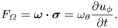
 $F_\varOmega$) is directly related to the boundary vorticity flux, by the expression
  $F_\varOmega = \boldsymbol { \sigma } \boldsymbol {\cdot } \boldsymbol { \omega }$ (Wu Reference Wu1995).
Recently, the boundary enstrophy flux has found a new application in the study of near-wall surface features. The boundary enstrophy flux gives a direct relationship between the skin-friction vector and the surface pressure (Liu et al. Reference Liu, Misaka, Asai, Obayashi and Wu2016; Chen, Liu & Wang Reference Chen, Liu and Wang2021), which leads to a new formula for the lift and drag force on a solid body in a viscous flow (Liu, Wang & He Reference Liu, Wang and He2017; Wu, Liu & Liu Reference Wu, Liu and Liu2018; Liu Reference Liu2021).
There is some ambiguity regarding the dynamics of vorticity. In particular, there are two alternative definitions of the vorticity current tensor in the fluid interior, as well as of the boundary vorticity flux (Terrington, Hourigan & Thompson Reference Terrington, Hourigan and Thompson2021). The traditional definitions are due to Lighthill (Reference Lighthill1963) and Panton (Reference Panton1984); however, an alternative definition of the vorticity current is provided by Huggins (Reference Huggins1970, Reference Huggins1971, Reference Huggins1994), while an alternative definition of the boundary vorticity flux was suggested by Lyman (Reference Lyman1990). There is no clear physical reason to prefer either definition (Terrington et al. Reference Terrington, Hourigan and Thompson2021), and, in general, one is free to use either definition. This leads to two alternative, but equally valid, dynamical interpretations of vorticity dynamics, which we refer to as the Lighthill–Panton (L–P) and Lyman–Huggins (L–H) interpretations, respectively.
The L–H interpretation of vorticity transport offers several advantages over the L–P interpretation (Terrington et al. Reference Terrington, Hourigan and Thompson2021). In particular, it more clearly illustrates the kinematic relationship between velocity and vorticity; it allows vorticity creation to be interpreted as an inviscid process; it offers a powerful control-surface analysis of three-dimensional flows; and it clearly illustrates how the solenoidal property of the vorticity field is maintained during vortex reconnections. It is therefore of great interest to determine whether the dynamics of enstrophy can be interpreted in a manner consistent with the L–H interpretation of vorticity dynamics.
This study extends both the L–P and L–H interpretations of vorticity dynamics to the dynamics of enstrophy. We demonstrate that each definition of the vorticity current tensor leads to a consistent set of definitions for the boundary vorticity flux, the boundary enstrophy flux, the enstrophy current, and the enstrophy dissipation term. Each set of definitions leads to an alternative dynamical interpretation of vorticity and enstrophy dynamics, which we call the L–P interpretation and the L–H interpretation, respectively. Importantly, the kinematic evolution of the enstrophy field is the same under each set of definitions, and it is only the dynamical interpretation of the motion that differs.
The structure of this article is as follows. First, in § 2, we review the dynamics of vorticity and enstrophy, and introduce the L–P and L–H interpretations of vorticity and enstrophy dynamics. Then, in § 3, we examine several example flows under both interpretations, to highlight the differences between each interpretation. Finally, concluding remarks are made in § 4.
2. Enstrophy dynamics
In this section, we introduce the L–P and L–H interpretations of vorticity and enstrophy dynamics. The structure of this section is as follows. First, in §§ 2.1 and 2.2, we review the dynamics of vorticity under the L–P and L–H definitions. Then, in § 2.3, we extend the L–P and L–H definitions to the dynamics of enstrophy. Finally, in § 2.4, we discuss the generation of enstrophy and vorticity on solid boundaries.
2.1. Vorticity dynamics
Consider an incompressible flow of a Newtonian fluid, which is governed by the momentum and continuity equations:
 \begin{gather} \frac{\partial{\boldsymbol{u}}}{\partial{t}} + \boldsymbol{u} \boldsymbol{\cdot} \boldsymbol{\nabla} \boldsymbol{u} ={-}\frac{1}{\rho} \boldsymbol{\nabla} p + \nu \boldsymbol{\nabla}^2 \boldsymbol{u}, \end{gather}
 \begin{gather} \boldsymbol{\nabla} \boldsymbol{\cdot} \boldsymbol{u} = 0,\end{gather}
where  $\boldsymbol {u}$ is the velocity,
  $p$ is the pressure and
  $\rho$ and
  $\nu$ are the fluid density and kinematic viscosity, respectively.
The Helmholtz equation, a transport equation for vorticity, is obtained by taking the curl of (2.1):
 \begin{equation} \frac{\partial{\boldsymbol{ \omega}}}{\partial{t}} + \boldsymbol{u} \boldsymbol{\cdot} \boldsymbol{\nabla} \boldsymbol{ \omega} = \boldsymbol{ \omega} \boldsymbol{\cdot} \boldsymbol{\nabla} \boldsymbol{u} + \nu \boldsymbol{\nabla}^2 \boldsymbol{ \omega}. \end{equation}
The left-hand side of (2.3) is the material derivative of vorticity, whereas the first term on the right-hand side describes the effects of vortex stretching and tilting. Finally, the last term on the right-hand side represents the effects of viscous diffusion.
Equation (2.3) can also be expressed as the divergence of a vorticity current tensor (Huggins Reference Huggins1970, Reference Huggins1971, Reference Huggins1994; Huggins & Bacon Reference Huggins and Bacon1980; Kolár Reference Kolár2003; Terrington et al. Reference Terrington, Hourigan and Thompson2021):
 \begin{equation} \frac{\partial{\boldsymbol{ \omega}}}{\partial{t}} ={-}\boldsymbol{\nabla} \boldsymbol{\cdot} \boldsymbol{\mathsf{J}},\end{equation}
where the vorticity current tensor,  $\boldsymbol{\mathsf{J}}$, is interpreted as follows: given two arbitrary unit vectors
  $\boldsymbol {\hat {a}}$ and
  $\boldsymbol {\hat {b}}$, the term
  $\boldsymbol {\hat {a}}\boldsymbol {\cdot }\boldsymbol{\mathsf{J}} \boldsymbol {\cdot } \boldsymbol {\hat {b}}$ describes the local flow rate of
  $\boldsymbol {\hat {b}}$ oriented vorticity in the
  $\boldsymbol {\hat {a}}$ direction. We remark that
  $\boldsymbol{\mathsf{J}}$ was previously referred to in Terrington et al. (Reference Terrington, Hourigan and Thompson2021) as the ‘vorticity flux tensor’. However, the term ‘vorticity flux’ can mean two different things. When referring to the tensor
  $\boldsymbol{\mathsf{J}}$, ‘vorticity flux’ refers to the rate of transport of vorticity across a boundary, analogous to the heat flux. However, ‘vorticity flux’ can also refer to the surface integral of normal vorticity, analogous to the magnetic flux (Greene Reference Greene1993). To avoid any confusion, we refer to
  $\boldsymbol{\mathsf{J}}$ as the ‘vorticity current tensor’, following Huggins (Reference Huggins1970, Reference Huggins1971, Reference Huggins1994).
Equation (2.4) shows that vorticity is a conserved quantity, and the total vorticity within a fluid volume can only change by the transport of vorticity across the outer boundary (Brøns et al. Reference Brøns, Thompson, Leweke and Hourigan2014; Terrington, Hourigan & Thompson Reference Terrington, Hourigan and Thompson2020, Reference Terrington, Hourigan and Thompson2022b). Specifically, for a stationary volume  $V$, the rate of change of volume-integrated vorticity is given by
 \begin{equation} \frac{\mathrm {\rm d} }{\mathrm {\rm d} t} \int_{V} \boldsymbol{ \omega} \,\mathrm{d} V ={-}\oint_{\partial V} \boldsymbol{\hat{n}} \boldsymbol{\cdot} \boldsymbol{\mathsf{J}} \,\mathrm{d} S,\end{equation}
where  $\boldsymbol {\hat {n}}$ is the unit normal directed out of the control volume.
The quantity  $\boldsymbol { \sigma } = \boldsymbol {\hat {n}} \boldsymbol {\cdot } \boldsymbol{\mathsf{J}}$ is known as the boundary vorticity flux (Lighthill Reference Lighthill1963; Wu & Wu Reference Wu and Wu1993, Reference Wu and Wu1996; Kolár Reference Kolár2003; Terrington et al. Reference Terrington, Hourigan and Thompson2021), which represents the rate at which vorticity is transported across the boundary, per unit area. Of particular importance, when
  $\partial V$ represents a solid boundary,
  $\boldsymbol { \sigma }$ describes the local vorticity creation rate per unit area on the boundary (Lighthill Reference Lighthill1963; Morton Reference Morton1984; Wu & Wu Reference Wu and Wu1993, Reference Wu and Wu1996; Terrington et al. Reference Terrington, Hourigan and Thompson2021).
The vorticity current tensor, as well as the boundary vorticity flux, cannot be unambiguously defined (Lyman Reference Lyman1990; Terrington et al. Reference Terrington, Hourigan and Thompson2021), and two competing definitions are often used in the literature. The original definition of the boundary vorticity flux was given by Lighthill (Reference Lighthill1963) and Panton (Reference Panton1984) as
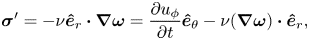
 \begin{equation} \boldsymbol{ \sigma}' ={-}\nu\boldsymbol{\hat{n}} \boldsymbol{\cdot} \boldsymbol{\nabla} \boldsymbol{ \omega},\end{equation}
which leads to the following definition of the vorticity current tensor:
 \begin{equation} \boldsymbol{\mathsf{J}}' = \boldsymbol{u} \boldsymbol{ \omega}- \boldsymbol{ \omega} \boldsymbol{u} - \nu \boldsymbol{\nabla} \boldsymbol{ \omega}. \end{equation}
However, Huggins (Reference Huggins1970, Reference Huggins1971, Reference Huggins1994) defines the vorticity current tensor as
 \begin{equation} \boldsymbol{\mathsf{J}} = \boldsymbol{u} \boldsymbol{ \omega}- \boldsymbol{ \omega} \boldsymbol{u} - \nu (\boldsymbol{\nabla} \boldsymbol{ \omega} -(\boldsymbol{\nabla} \boldsymbol{ \omega})^{\mathrm T}),\end{equation}
whereas Lyman (Reference Lyman1990) provides an alternative definition of the boundary vorticity flux, which is consistent with Huggins’ definition of the vorticity current tensor:
 \begin{equation} \boldsymbol{ \sigma} = \nu\boldsymbol{\hat{n}} \times (\boldsymbol{\nabla} \times \boldsymbol{ \omega}).\end{equation}
 Before continuing, we must clarify some of the terminology. In particular, we have previously referred to the tensor  $\boldsymbol{\mathsf{J}}$ as the L–H tensor. However, as pointed out by Eyink (Reference Eyink2021), this double attribution is not appropriate, because Huggins introduced the vorticity current tensor over two decades before Lyman introduced the boundary vorticity flux. Therefore, the tensor
  $\boldsymbol{\mathsf{J}}$ is referred to as the Huggins vorticity current tensor, whereas the vector
  $\boldsymbol { \sigma }$ is referred to as the Lyman boundary vorticity flux. We refer to the vector
  $\boldsymbol { \sigma }'$ and tensor
  $\boldsymbol{\mathsf{J}}'$ as the L–P boundary vorticity flux and the L–P vorticity current tensor, respectively.
Each definition of the vorticity current tensor, and the corresponding boundary vorticity flux, leads to an alternative interpretation of vorticity dynamics: the L–P interpretation, based on the L–P boundary vorticity flux and vorticity current tensor; and the L–H interpretation, based on Huggins’ vorticity current tensor and Lyman's boundary vorticity flux. The present work extends the L–P and L–H interpretations of vorticity dynamics to include the dynamics of enstrophy.
2.2. Alternative interpretations of vorticity dynamics
Which of the two competing interpretations (L–P and L–H) should be used to describe the generation and transport of vorticity has been controversial. In particular, Wu & Wu (Reference Wu and Wu1993, Reference Wu and Wu1998) support the L–P interpretation, whereas Eyink (Reference Eyink2008) and Eyink, Gupta & Zaki (Reference Eyink, Gupta and Zaki2020) prefer the L–H interpretation. Other authors (Lyman Reference Lyman1990; Kolár Reference Kolár2003) accept the notion that either definition may be used. We have recently argued that it is appropriate to use either definition (Terrington et al. Reference Terrington, Hourigan and Thompson2021), with each definition offering a different, but equally valid, interpretation of vorticity dynamics. In this section, we summarise some key points surrounding the controversy over the definition of the boundary vorticity flux. For further details, readers are referred to our previous discussion (Terrington et al. Reference Terrington, Hourigan and Thompson2021).
Wu & Wu (Reference Wu and Wu1993, Reference Wu and Wu1998) present two arguments as to why the L–H definitions are inappropriate, and therefore the L–P definitions are the only correct interpretation. First, Lyman's definition of the boundary vorticity flux is equal to the viscous acceleration of a boundary fluid element, and therefore includes viscous stresses applied to this element from both the fluid and the wall. Hence, Wu & Wu (Reference Wu and Wu1993) argue that this cannot represent a vorticity creation process occurring solely on the boundary. However, both the L–P and L–H definitions are related to gradients in the shear stress (vorticity gradients) and, therefore, neither definition can represent the sole action of the boundary on boundary fluid elements (Terrington et al. Reference Terrington, Hourigan and Thompson2021). Therefore, this argument provides no reason to prefer the L–P definition over the L–H interpretation.
Wu & Wu (Reference Wu and Wu1998) provide a second argument in support of the L–P definition. They derive an expression for the rate of change of circulation at an open control surface, which is related to the L–P definition of the boundary vorticity flux. However, in their derivation, they neglect a term related to the curvature of vortex lines, assuming the curvature of the boundary curve  $C$ can always be made much greater than the curvature of vortex lines. However, the curvature of
  $C$ does not appear in this equation, so the vortex-line curvature term cannot be neglected (Terrington et al. Reference Terrington, Hourigan and Thompson2021). When this term is not neglected, Lyman's definition, rather than the L–P definition, is obtained.
There does not appear to be a clear physical reason to prefer either the L–P or L–H interpretations (Terrington et al. Reference Terrington, Hourigan and Thompson2021). Instead, each definition offers a different, but equally valid, dynamical interpretation of the evolution of the vorticity field. While at first this may appear surprising, one must remember that the vorticity field is obtained from the velocity field by a purely kinematic operation (Lyman Reference Lyman1990). Changes to the velocity field are governed by the Navier–Stokes equations, which are a statement of the conservation of linear momentum. Essentially, the redistribution of linear momentum by pressure and viscous forces produces corresponding changes to both the velocity and vorticity fields. It is often convenient to visualise and interpret fluid motions by the evolution of the vorticity field, rather than the velocity field. One then treats vorticity as the primary variable, and either the L–H or L–P definitions may be used to understand the generation and redistribution of vorticity in the flow.
We have previously found that for many flows, the L–H interpretation offers the following advantages over the L–P interpretation (Terrington et al. Reference Terrington, Hourigan and Thompson2021). First, Lyman's flux is equal to the viscous acceleration of boundary fluid elements and, therefore, more clearly illustrates the kinematic relationship between velocity and vorticity. Second, Lyman's definition of the boundary vorticity flux allows vorticity generation to be described as an inviscid process, generalising Morton's (Reference Morton1984) interpretation of vorticity creation to three-dimensional flows. Third, Huggins’ vorticity current tensor can be related to the transport of circulation in any two-dimensional reference surface, allowing a powerful control-surface analysis of three-dimensional vortical flows. Finally, the L–H interpretation clearly illustrates how the kinematic condition that vortex lines do not end inside the fluid is maintained during viscous processes such as vortex reconnection (Terrington et al. Reference Terrington, Hourigan and Thompson2021), or the connection of a vortex ring to a free surface (Terrington, Hourigan & Thompson Reference Terrington, Hourigan and Thompson2022a). In addition, Eyink (Reference Eyink2021) has shown that the Huggins tensor leads to a generalised Josephson–Anderson relation between the drag on a finite solid body and the vorticity flux. The numerous benefits offered by the L–H interpretation of vorticity dynamics motivate us to develop the corresponding L–H interpretation of enstrophy dynamics, which is presented in § 2.3.
Recently, Wang, Eyink & Zaki (Reference Wang, Eyink and Zaki2022) have emphasised that the two expressions  $\boldsymbol { \sigma }' = -\nu \boldsymbol {\hat {n}} \boldsymbol {\cdot } \boldsymbol {\nabla } \boldsymbol { \omega }$ and
  $\boldsymbol { \sigma } = \nu \boldsymbol {\hat {n}} \times (\boldsymbol {\nabla } \times \boldsymbol { \omega })$ measure slightly different things in general, and therefore in some contexts only one of these definitions may be appropriate. We stress that either definition may always be adopted as representing the local flow rate of vorticity across a boundary. In some contexts, however, these expressions are related to some other quantity, such as the total force and moment on a closed boundary (Wu & Wu Reference Wu and Wu1993, Reference Wu and Wu1996), and these relationships may only hold for one definition of the boundary vorticity flux.
2.3. Enstrophy dynamics
Although vorticity is a conserved quantity, this does not mean the total rotational motion within a fluid remains constant. In particular, cross-diffusive annihilation of opposite-signed vorticity can occur (Morton Reference Morton1984), which leads to a reduction in the kinetic energy contained in vortical structures, without a reduction in the volume-integrated vorticity. Enstrophy, however, measures the local fluid rotation without considering the direction of rotation, and therefore the volume-integrated enstrophy provides a measure of the total rotational motion within a fluid flow. In this subsection, we extend the L–P and L–H interpretations of vorticity dynamics to the dynamics of enstrophy.
A transport equation for enstrophy can be derived from (2.4), by taking the dot product with vorticity (Wu Reference Wu1995; Chen et al. Reference Chen, Liu and Wang2021):
 \begin{equation} \frac{\partial{\varOmega}}{\partial{t}} ={-}(\boldsymbol{\nabla} \boldsymbol{\cdot} \boldsymbol{\mathsf{J}} )\boldsymbol{\cdot} \boldsymbol{ \omega}={-}\boldsymbol{\nabla} \boldsymbol{\cdot} (\boldsymbol{\mathsf{J}} \boldsymbol{\cdot} \boldsymbol{ \omega}) + \boldsymbol{\mathsf{J}} \boldsymbol{:} \boldsymbol{\nabla} \boldsymbol{ \omega}, \end{equation}
where  $\boldsymbol {:}$ denotes twice contraction (in Cartesian tensor notation,
  $\boldsymbol{\mathsf{J}} \boldsymbol {:} \boldsymbol {\nabla } \boldsymbol { \omega } = J_{ij} \partial \omega _j/\partial {x_i}$).
As the advection and vortex stretching/tilting terms in both the L–P and Huggins’ vorticity current tensors are the same, we can split the vorticity current tensor into inviscid and viscous parts:
 \begin{equation} \boldsymbol{\mathsf{J}} = \boldsymbol{u} \boldsymbol{ \omega} - \boldsymbol{ \omega} \boldsymbol{u} + \boldsymbol{\mathsf{J}}_{\nu}, \end{equation}
where  $\boldsymbol{\mathsf{J}}'_{\nu } = -\nu \boldsymbol {\nabla } \boldsymbol { \omega }$ for the L–P tensor, and
  $\boldsymbol{\mathsf{J}}_{\nu } = -\nu (\boldsymbol {\nabla } \boldsymbol { \omega } - (\boldsymbol {\nabla } \boldsymbol { \omega })^{\mathrm T})$ for the Huggins tensor. Using this decomposition, (2.10) becomes
 \begin{equation} \frac{\partial{\varOmega}}{\partial{t}} + \boldsymbol{u} \boldsymbol{\cdot} \boldsymbol{\nabla} \varOmega = \boldsymbol{ \omega} \boldsymbol{\cdot} (\boldsymbol{\nabla} \boldsymbol{u}) \boldsymbol{\cdot} \boldsymbol{ \omega} - \boldsymbol{\nabla} \boldsymbol{\cdot} (\boldsymbol{\mathsf{J}}_{\nu} \boldsymbol{\cdot} \boldsymbol{ \omega}) + \boldsymbol{\mathsf{J}}_{\nu} \boldsymbol{:} \boldsymbol{\nabla} \boldsymbol{ \omega}. \end{equation}
The left-hand side of 2.12 is the material derivative of enstrophy, whereas the first term on the right-hand side describes the vortex stretching effect. The term  $-\boldsymbol {\nabla } \boldsymbol {\cdot } (\boldsymbol{\mathsf{J}}_{\nu } \boldsymbol {\cdot } \boldsymbol { \omega })$ describes the diffusive transport of enstrophy, and the final term,
  $\boldsymbol{\mathsf{J}}_{\nu } \boldsymbol {:} \boldsymbol { \omega }$, describes the viscous dissipation of enstrophy.
The viscous diffusion term can also be written as the divergence of an enstrophy current vector,
 \begin{equation} \boldsymbol{Q} = \boldsymbol{\mathsf{J}}_{\nu} \boldsymbol{\cdot} \boldsymbol{ \omega},\end{equation}
where  $\boldsymbol {\hat {n}} \boldsymbol {\cdot } \boldsymbol {Q}$ describes the local flow-rate of enstrophy in the
  $\boldsymbol {\hat {n}}$ direction. This implies that the boundaries of a fluid domain can act as a source or sink of enstrophy, with the boundary enstrophy flux given by
 \begin{equation} F_{\varOmega} = \boldsymbol{\hat{n}} \boldsymbol{\cdot} \boldsymbol{Q} = \boldsymbol{ \omega} \boldsymbol{\cdot} (\boldsymbol{\hat{n}} \boldsymbol{\cdot} \boldsymbol{\mathsf{J}}_{\nu}) = \boldsymbol{ \omega} \boldsymbol{\cdot} \boldsymbol{ \sigma}. \end{equation}
The physical interpretation of (2.14) is quite simple: when the vorticity generated on or diffused out of a boundary is of the same sign as the boundary vorticity, the local enstrophy is enhanced by the creation of vorticity on the boundary (Wu Reference Wu1995). However, when the vorticity created on the boundary is of opposite sign to the boundary vorticity, enstrophy is reduced as existing vorticity cross-annihilates with the newly generated vorticity.
As with the viscous part of the vorticity current tensor, both the enstrophy diffusion and dissipation terms cannot be unambiguously defined, and depend on which definition of the vorticity current tensor is used. When the L–P definition is used, the viscous dissipation term becomes
 \begin{equation} D' = \boldsymbol{\mathsf{J}}'_{\nu} \boldsymbol{:} \boldsymbol{\nabla} \boldsymbol{ \omega} ={-}\nu \boldsymbol{\nabla} \boldsymbol{ \omega} \boldsymbol{:} \boldsymbol{\nabla} \boldsymbol{ \omega}, \end{equation}
whereas the enstrophy–current vector becomes
 \begin{equation} \boldsymbol{Q}' = \boldsymbol{\mathsf{J}}'_\nu \boldsymbol{\cdot} \boldsymbol{ \omega} ={-}\nu(\boldsymbol{\nabla} \boldsymbol{ \omega}) \boldsymbol{\cdot} \boldsymbol{ \omega} ={-}\nu \boldsymbol{\nabla} \varOmega, \end{equation}
and the boundary enstrophy flux is
 \begin{equation} F'_{\varOmega} = \boldsymbol{ \omega} \boldsymbol{\cdot} \boldsymbol{ \sigma}' ={-}\nu \boldsymbol{ \omega} \boldsymbol{\cdot}(\boldsymbol{\hat{n}} \boldsymbol{\cdot} \boldsymbol{\nabla} \boldsymbol{ \omega}) ={-}\nu \boldsymbol{\hat{n}} \boldsymbol{\cdot} \boldsymbol{\nabla} \varOmega. \end{equation}
Equations (2.15)–(2.17), as well as (2.6) and (2.7), collectively form the L–P interpretation of enstrophy and vorticity dynamics. These are the usual definitions of the viscous dissipation term and the boundary enstrophy flux, and have been used by Wu (Reference Wu1995), Liu et al. (Reference Liu, Misaka, Asai, Obayashi and Wu2016) and Chen et al. (Reference Chen, Liu and Wang2021).
An alternative definition of the viscous dissipation and diffusion terms is obtained when one uses Huggins’ definition of the vorticity current tensor:
 \begin{gather} D = \boldsymbol{\mathsf{J}}_{\nu} \boldsymbol{:} \boldsymbol{\nabla} \boldsymbol{ \omega} = \nu ( (\boldsymbol{\nabla} \boldsymbol{ \omega})^{\mathrm T} - \boldsymbol{\nabla} \boldsymbol{ \omega}) \boldsymbol{:} \boldsymbol{\nabla} \boldsymbol{ \omega} ={-}\nu (\boldsymbol{\nabla}\times \boldsymbol{ \omega}) \boldsymbol{\cdot} (\boldsymbol{\nabla} \times \boldsymbol{ \omega}), \end{gather}
 \begin{gather} \boldsymbol{Q} = \boldsymbol{\mathsf{J}}_{\nu} \boldsymbol{\cdot} \boldsymbol{ \omega} = \nu\boldsymbol{ \omega} \boldsymbol{\cdot} (\boldsymbol{\nabla} \boldsymbol{ \omega} - (\boldsymbol{\nabla} \boldsymbol{ \omega})^{\mathrm T}) ={-}\nu \boldsymbol{ \omega} \times (\boldsymbol{\nabla} \times \boldsymbol{ \omega}),\end{gather}
 \begin{gather} F_{\varOmega} = \boldsymbol{ \omega} \boldsymbol{\cdot} \boldsymbol{ \sigma} = \nu \boldsymbol{ \omega} \boldsymbol{\cdot} (\boldsymbol{\hat{n}} \times(\boldsymbol{\nabla} \times \boldsymbol{ \omega})) ={-}\nu \boldsymbol{\hat{n}} \boldsymbol{\cdot} [ \boldsymbol{ \omega} \times (\boldsymbol{\nabla} \times \boldsymbol{ \omega})].\end{gather}
Equations (2.18)–(2.20), as well as (2.9) and (2.8), collectively form the L–H interpretation of enstrophy dynamics. To the best of the authors’ knowledge, these definitions have not previously been considered as an alternative definition of the enstrophy generation, transport and diffusion terms.
As with the dynamics of vorticity, both the L–P and L–H definitions give the same kinematic evolution of the enstrophy field through (2.12). It is only the dynamical interpretation of this motion, including the local enstrophy generation rate on the boundary, the local flow rate of enstrophy in the fluid interior and the local enstrophy dissipation rate, that differs between the two definitions. Enstrophy, much the same as vorticity, is obtained from the velocity field by a purely kinematic relationship and, therefore, changes to the enstrophy field are a consequence of the redistribution of linear momentum throughout the flow. The L–H and L–P definitions provide alternative dynamical interpretations of the effects of the transport of linear momentum on the evolution of the vorticity and enstrophy fields.
2.4. The inviscid mechanism of vorticity and enstrophy creation
One of the main advantages of the L–H interpretation is that vorticity creation on an interface or boundary can be interpreted as an inviscid process (Morton Reference Morton1984; Terrington et al. Reference Terrington, Hourigan and Thompson2021, Reference Terrington, Hourigan and Thompson2022b). Therefore, under the L–H interpretation, enstrophy creation should also be considered an inviscid process. In this subsection, we discuss the inviscid theory of vorticity and enstrophy creation.
Using the tangential momentum equation, we obtain the following expression for the boundary vorticity flux (Lyman Reference Lyman1990; Terrington et al. Reference Terrington, Hourigan and Thompson2021)
 \begin{equation} \boldsymbol{ \sigma} ={-}\boldsymbol{\hat{n}} \times \left[\frac{\mathrm {\rm d} \boldsymbol{u}}{\mathrm {\rm d} t} + \boldsymbol{\nabla} \left( \frac{p}{\rho}\right)\right], \end{equation}
where  $\mathrm {d}\boldsymbol {u}/\mathrm d t$ is the material derivative of velocity. The right-hand side of (2.21) represents the relative acceleration between the fluid and the solid that would occur in the absence of any viscous acceleration (Morton Reference Morton1984; Terrington et al. Reference Terrington, Hourigan and Thompson2021), due to either tangential acceleration of the boundary or tangential pressure gradients. As first discussed by Morton (Reference Morton1984), this inviscid relative acceleration would produce a velocity discontinuity, which is interpreted as a sheet of vorticity on the boundary (Morton Reference Morton1984; Terrington et al. Reference Terrington, Hourigan and Thompson2021, Reference Terrington, Hourigan and Thompson2022b). Viscous forces are responsible for the redistribution of vorticity into the fluid after it has been generated, thereby maintaining the no-slip boundary condition (Morton Reference Morton1984; Terrington et al. Reference Terrington, Hourigan and Thompson2021).
Using (2.20), the boundary enstrophy flux is related to the boundary vorticity flux:
 \begin{equation} F_\varOmega ={-}\boldsymbol{ \omega} \boldsymbol{\cdot} \left(\boldsymbol{\hat{n}} \times \left[\frac{\mathrm {\rm d} \boldsymbol{u}}{\mathrm {\rm d} t} + \boldsymbol{\nabla} \left( \frac{p}{\rho}\right)\right]\right). \end{equation}
Therefore, the inviscid creation of vorticity on a boundary, by either tangential acceleration of the boundary, or a tangential pressure gradient, can also result in either the creation or destruction of enstrophy on the boundary, depending on the relative orientations of the boundary vorticity and the boundary vorticity flux.
Under the L–P interpretation, however, the inviscid theory of vorticity creation does not apply. An additional viscous term appears in the expressions for the boundary vorticity flux and boundary enstrophy flux (Wu & Wu Reference Wu and Wu1993):
 \begin{gather} \boldsymbol{ \sigma}' ={-}\boldsymbol{\hat{n}} \times \left[\frac{\mathrm {\rm d} \boldsymbol{u}}{\mathrm {\rm d} t} + \boldsymbol{\nabla} \left( \frac{p}{\rho}\right)\right] - \nu(\boldsymbol{\nabla} \boldsymbol{ \omega})\boldsymbol{\cdot} \boldsymbol{\hat{n}},\end{gather}
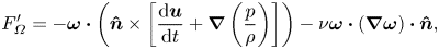 \begin{gather} F_\varOmega' ={-}\boldsymbol{ \omega} \boldsymbol{\cdot} \left(\boldsymbol{\hat{n}} \times \left[\frac{\mathrm {\rm d} \boldsymbol{u}}{\mathrm {\rm d} t} + \boldsymbol{\nabla} \left( \frac{p}{\rho}\right)\right]\right) - \nu \boldsymbol{ \omega} \boldsymbol{\cdot} (\boldsymbol{\nabla} \boldsymbol{ \omega})\boldsymbol{\cdot} \boldsymbol{\hat{n}},\end{gather}
Therefore, in addition to tangential boundary acceleration and tangential pressure gradients, vorticity and enstrophy are also generated by a purely viscous mechanism, related to the distribution of wall shear-stress on the boundary (Wu & Wu Reference Wu and Wu1993). For high-Reynolds-number flows, this viscous term is usually small, except for local regions of high surface curvature, or near singular points in the wall-shear stress (Wu & Wu Reference Wu and Wu1993).
We stress that the additional viscous terms do not occur under the L–H interpretation. Therefore, L–H offers a conceptually more elegant interpretation of vorticity and enstrophy generation on a boundary, where vorticity, and therefore enstrophy, is only generated by an inviscid relative acceleration between the solid boundary and the wall, driven by either tangential pressure gradients or tangential acceleration of the boundary.
3. Examples
We now consider several example flows, examining each flow under the L–H and L–P interpretations to highlight the differences between the two interpretations. The first two examples we consider, Kida's straight jet flow and the Stokes flow over an impulsively rotated sphere, are highly viscous flows, in which inertial effects are small. These examples show remarkable differences between the L–H and L–P interpretations: the flow structures associated with strong enstrophy dissipation may differ between the two interpretations, and the total enstrophy creation on a solid boundary, as well as the total enstrophy dissipation in the fluid interior, may also differ between the two definitions. The third example we consider is the inertial flow over a rotating sphere, which suggests that for highly inertial flows, the differences between the two interpretations of enstrophy dynamics are generally small.
3.1. Kida's straight jet flow
The first example we consider is Kida and Takaoka's (Reference Kida and Takaoka1991) straight-jet flow, which is a two-dimensional model of symmetrical vortex reconnection. We have previously investigated the dynamics of vorticity in this flow under the L–H interpretation (Terrington et al. Reference Terrington, Hourigan and Thompson2021), and found that this interpretation provides an elegant description of the vortex connection mechanism. In particular, the breaking open and subsequent reconnection of vortex lines are attributed to a single physical process, which clearly explains how the kinematic condition that vortex filaments do not end inside the fluid is maintained throughout the interaction.
In this section, we discuss the dynamics of enstrophy for the straight jet flow, under both the L–P and L–H interpretations. In particular, we find that the flow structures associated with strong enstrophy dissipation differ between the two interpretations, and that the diffusion of enstrophy under L–H more closely resembles the typical interpretation of the vortex reconnection process.
The straight-jet flow is a family of analytic solutions to the Navier–Stokes equations, with velocity and vorticity given by Kida & Takaoka (Reference Kida and Takaoka1991):
 \begin{gather} \boldsymbol{u} = ({-}A x, 0, A z + u_3(x,y,t)), \end{gather}
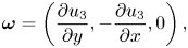 \begin{gather} \boldsymbol{ \omega} = \left(\frac{\partial{u_3}}{\partial{y}},-\frac{\partial{u_3}}{\partial{x}} ,0\right), \end{gather}
 \begin{gather} u_3(x,y,t) = \frac{u_0 r_0^2 \mathrm{e}^{{-}2At}}{\sigma_1\sigma_2} \left[ \exp{} \left[-\frac{(x-a\mathrm{e}^{{-}At})^2}{\sigma_1^2} - \frac{y^2}{\sigma_2^2}\right] + \exp{} \left[-\frac{(x +a\mathrm{e}^{{-}At})^2}{\sigma_1^2} - \frac{y^2}{\sigma_2^2}\right]\right], \end{gather}
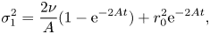 \begin{gather} \sigma_1^2 = \frac{2\nu}{A} (1-\mathrm{e}^{{-}2At}) + r_0^2\mathrm{e}^{{-}2At}, \end{gather}
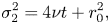 \begin{gather} \sigma_2^2 = 4\nu t + r_0^2, \end{gather}
where  $A$,
$A$,  $r_0$,
  $a$ and
  $u_0$ are constants. The vorticity field (3.2) is essentially a two-dimensional vector field, and therefore vortex lines lie entirely within the
  $x$–
$x$– $y$ plane. Moreover, each vortex line is also a level surface of the scalar field
  $u_3$.
We consider a single case with parameters  $A=1$,
  $\nu = 0.5$,
  $r_0= 0.5$,
  $u_0 = 1$ and
  $a = 1$, which were chosen to provide a clear example of vortex reconnection. Vortex lines (contours of
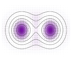
  $u_3$) are plotted at a selection of flow times in figure 1, and a transient animation is provided in supplementary movie 1 available at https://doi.org/10.1017/jfm.2023.95. This flow initially features three singular points (where
  $\boldsymbol { \omega } = \boldsymbol {0}$): two ‘O’-points, labelled
  $O_1$ and
  $O_2$, and one ‘X’-point, labelled
  $X$. At the critical time
  $t \approx 0.5058$, the singular points merge into a single ‘O’-point.
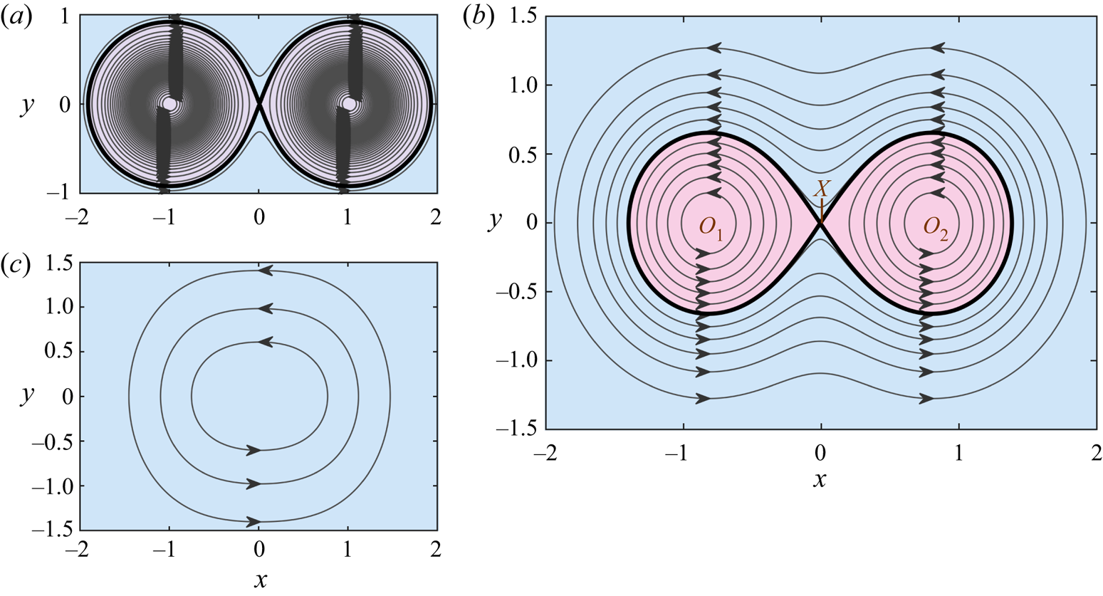
Figure 1. Vortex lines in the  $x$–
$x$– $y$ plane (contours of
  $u_3$), at flow times (a)
  $t = 0$, (b)
  $t = 0.2$ and (c)
  $t = 0.6$, for Kida's straight jet flow. Vortex lines are colour coded by whether they enclose only a single ‘O’-point (pink) or the entire system of two ‘O’-points and one ‘X’-point (blue).
Following the terminology used by Melander & Hussain (Reference Melander and Hussain1994), each vortex line in figure 1(b) lies in one of three islands: the ‘inner islands’ associated with  $O_1$ and
  $O_2$, which correspond to the pink shaded regions; and the outer island, which corresponds to the blue shaded region. The strength of each island is measured by the circulation, which is defined as the integral of normal vorticity along a curve that intersects each vortex line in the island precisely once (Greene Reference Greene1993; Melander & Hussain Reference Melander and Hussain1994). Note that the island circulation is usually referred to as the ‘vorticity flux’, by analogy with the magnetic flux (Greene Reference Greene1993; Melander & Hussain Reference Melander and Hussain1994). However, because the term ‘vorticity flux’ may be confused with the boundary vorticity flux, we shall refer to this quantity as the circulation.
Figure 2 presents the variation of the island circulations against time. The circulation associated with the inner islands decreases monotonically, until it becomes zero at the critical time  $t \approx 0.5058$. The circulation associated with the outer island initially increases, reaches a maximum value at
  $t \approx 0.24$ and subsequently decreases. The transient behaviour of the island circulations can be understood by considering the topological changes to the vortex lines that occur at the singular points (Greene Reference Greene1993; Melander & Hussain Reference Melander and Hussain1994). Specifically, the annihilation of circulation occurs at each ‘O’-point, resulting in the continual loss of circulation from the inner islands. Vortex reconnection occurs at the ‘X’-point, and transfers circulation from the inner island to the outer island. This produces the initial increase in the circulation associated with the outer island.
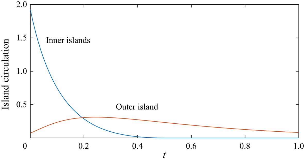
Figure 2. Time history of the circulation associated with the inner and outer islands.
We have previously analysed the diffusion of vorticity near the singular points, and shown that the L–H definition of the vorticity current tensor leads to an elegant interpretation of vortex reconnection at the ‘X’-point, and of the annihilation of circulation at the ‘O’-points (Terrington et al. Reference Terrington, Hourigan and Thompson2021). We now consider the dynamics of enstrophy in this flow under both the L–P and L–H interpretations.
Figure 3 presents colour plots of the enstrophy dissipation ( $D$) and vectors of the enstrophy current (
 $\boldsymbol {Q}$), as well as vortex lines, using (a) the L–H and (b) the L–P definitions, at
  $t = 0.2$. Although the total enstrophy dissipation is equal under each interpretation,
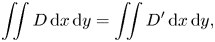 \begin{equation} \iint D \,{{\rm d} x} \, {{\rm d} y} = \iint D' \, {{\rm d} x} \,{{\rm d} y}, \end{equation}
the spatial distribution of enstrophy dissipation differs between each definition. Under the L–P definition, enstrophy dissipation is concentrated near the three singular points,  $O_1$,
  $O_2$ and
  $X$, whereas under the L–H interpretation, enstrophy dissipation is only concentrated near
  $O_1$ and
  $O_2$, with relatively low dissipation occurring at
  $X$.
$X$.

Figure 3. Colour plot indicating the enstrophy dissipation ( $D$), overlaid with vectors of the enstrophy current (
 $\boldsymbol {Q}$) and vortex lines (contours of
  $u_3$), at
  $t = 0.2$, under (a) the L–H interpretation and (b) the L–P interpretation.
Therefore, under L–P, both the reconnection of vorticity at  $X$ and the annihilation of circulation at
  $O_1$ and
  $O_2$ are associated with increased enstrophy dissipation, whereas under L–H, only the annihilation of circulation at
  $O_1$ and
  $O_2$ is associated with increased enstrophy dissipation. Vortex reconnection at
  $X$ is not associated with strong enstrophy dissipation under L–H. This is reasonable, since vortex reconnection simply represents the transfer of circulation across the reconnection point, whereas circulation annihilation represents the complete removal of vorticity (and therefore enstrophy) from the flow.
Figure 3 also reveals that the enstrophy currents are different under each definition. The most striking differences are seen near the connection point, which is illustrated more clearly in figure 4. Under L–H (figure 4a), the enstrophy current is always perpendicular to vortex lines, and therefore enstrophy cannot be transported along a vortex line. Moreover, the direction of the enstrophy current matches the perceived motion of vortex lines during the reconnection process, where vortex lines passing across the  $x$-axis are transported towards the connection point, whereas vortex lines intersecting the
  $y$-axis are transported away from the connection point. The enstrophy current vectors in figure 4(a) support this interpretation.
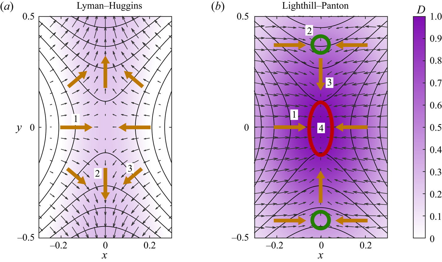
Figure 4. Closeup of figure 3, showing the enstrophy current and enstrophy dissipation near the connection point, under (a) the L–H and (b) the L–P interpretations. In panel (a), label 1 denotes the enstrophy transport towards the connection point; label 2 denotes the enstrophy transport away from the connection point; and label 3 marks where the enstrophy current matches the apparent motion of the vortex lines. In panel (b), label 1 denotes the enstrophy transport towards the connection point; label 2 denotes the enstrophy transport towards the symmetry plane; label 3 denotes the enstrophy transport towards the connection point; and label 4 denotes the enstrophy dissipation near the connection point.
Under L–P (figure 4b), however, enstrophy is transported towards the connection point in all directions, which is balanced by elevated enstrophy dissipation near the connection point. Moreover, the mechanism responsible for the increase in enstrophy at the  $y$-axis differs between the two interpretations. Specifically, the enstrophy at the locations indicated by green circles in figure 4(b) increases as vortex lines are reconnected across the
  $y$-axis. Under the L–P interpretation, this is attributed to the transport of enstrophy towards the
  $y$-axis in the
  $x$-direction, which, unlike the L–H interpretation, does not match the perceived motion of vortex lines under the usual interpretation of vortex reconnection.
3.2. Stokes flow over rotating sphere
The second example we consider is the Stokes flow driven by an impulsively started rotating sphere. In this example, the total enstrophy generation on the surface of the sphere, as well as the total enstrophy dissipation in the fluid interior, differ between the L–H and L–P interpretations. However, the total rate-of-change of enstrophy (including both enstrophy generation and dissipation) is the same for both definitions. Under L–H, the flow approaches a steady state where the generation, diffusion and dissipation of enstrophy are zero. Under L–P, however, the steady-state flow features continuous generation of enstrophy on the sphere, which is balanced by the continuous dissipation of enstrophy in the fluid interior.
The Stokes approximation allows the generation and dissipation of enstrophy to be isolated from the advection and vortex stretching terms. We consider the following transport equations for the ‘velocity’ field:
 \begin{equation} \frac{\partial{\boldsymbol{u}}}{\partial{t}} ={-}\boldsymbol{\nabla}\left(\frac{p}{\rho}\right) + \nu \boldsymbol{\nabla}^2 \boldsymbol{u}. \end{equation}
As shown in figure 5, we consider a sphere of radius  $R$, which is rotated with angular velocity
  $\boldsymbol {W} = W \boldsymbol {\hat {e}}_z$. Using a spherical coordinate system
  $(r,\theta,\phi$), the following transformation
 \begin{gather} u_r(r,\theta,t) = u_\theta(r,\theta,t) = p(r,\theta,t) = 0, \end{gather}
 \begin{gather} u_{\phi}(r,\theta,t) = W r \sin \theta f(\hat{r},\tau), \end{gather}
 \begin{gather} \hat{r} = r/R, \end{gather}
 \begin{gather} \tau = t/(R^2/\nu), \end{gather}
reduces (3.7) to a one-dimensional partial differential equation,
 \begin{equation} \frac{\partial{f}}{\partial{\tau}} = \frac{4}{\hat{r}}\frac{\partial{f}}{\partial{\hat{r}}} + \frac{\partial^2 f}{\partial \hat{r}^2}, \end{equation}
which has the following initial and boundary conditions for an impulsively started sphere:
 \begin{gather} f(1,\tau) = 1, \end{gather}
 \begin{gather} f(\hat{r},0) = 0. \end{gather}
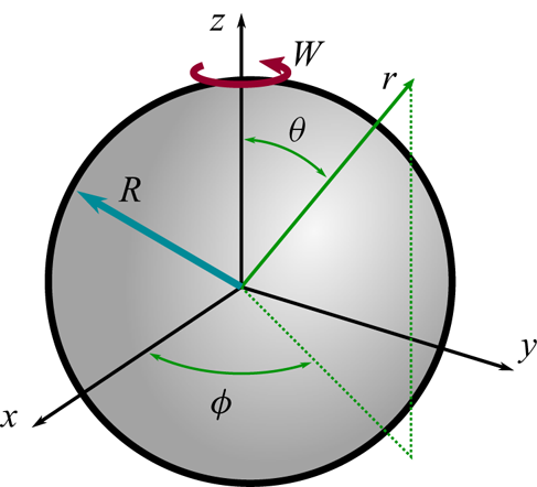
Figure 5. Geometry and spherical coordinate system  $(r,\theta,\phi )$ for the Stokes flow over an impulsively rotated sphere.
In this work, (3.9) and (3.10) are solved using a finite difference method. The semi-infinite domain in  $\hat {r}$ is transformed to a finite domain using the following transformation:
 \begin{equation} \hat{z} = \frac{\hat{r}-1}{\hat{r}+1}, \end{equation}
where  $0 \leq \hat {z} \leq 1$. Equation (3.9) is transformed into (
 $\tau,\hat {z}$) coordinates, and then discretised using a centred time centred space (CTCS) finite difference scheme. A regular grid containing
  $n_z = 1000$ points was used in the
  $\hat {z}$ direction, with a constant timestep of
  $\Delta \tau = 0.00001$. Using a larger timestep of
  $\Delta \tau = 0.0001$, or increasing the number of gridpoints to
  $n_z = 2000$, results in changes to the solution of less than
  $0.01\,\%$ at
  $\tau = 0.1$ and
  $\tau = 1$, confirming that a grid-independent result is obtained.
The vorticity and enstrophy fields for this flow are presented in figure 6, and an animation is provided in supplementary movie 2. On the initial rotation of the sphere, a finite quantity of vorticity is generated on the solid boundary and is immediately diffused into the fluid. A uniform vorticity field corresponding to pure rotation is also generated in the solid body, so that vortex lines are closed loops passing through both the solid and the fluid. During the transient evolution, vorticity and enstrophy in the fluid gradually diffuse away from the solid boundary, approaching a steady state given by
 \begin{gather} f(\hat{r},\infty) = 1/\hat{r}^3, \end{gather}
 \begin{gather} \omega_r(\hat{r},\infty) = 2W \cos \theta/\hat{r}^3, \end{gather}
 \begin{gather} \omega_\theta(\hat{r},\infty) = W \sin \theta/\hat{r}^3, \end{gather}
 \begin{gather} \varOmega = (4 \cos^2 \theta + \sin^2 \theta) W^2/\hat{r}^6. \end{gather}
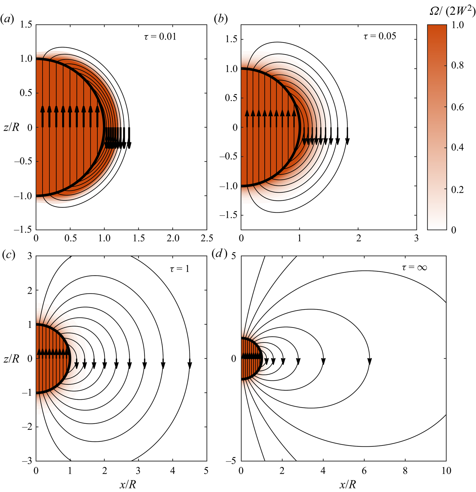
Figure 6. Colour plot indicating the dimensionless enstrophy, overlaid with vortex lines, for a selection of dimensionless flow times. The vorticity and enstrophy fields for solid body rotation in the sphere are also included.
We have previously discussed the dynamics of vorticity for this flow (Terrington et al. Reference Terrington, Hourigan and Thompson2021). Under L–H, the boundary vorticity flux is given by (2.21)
 \begin{equation} \boldsymbol{\sigma} = \nu \boldsymbol{\hat{e}}_r \times (\boldsymbol{\nabla} \times \boldsymbol{ \omega}) = \frac{\partial{u_\phi}}{\partial{t}} \boldsymbol{\hat{e}}_\theta, \end{equation}
and is zero apart from the initial impulsive acceleration. Therefore, all vorticity is generated during the initial rotation of the sphere, and the total vorticity in the fluid remains constant thereafter. In the steady-state flow, the vorticity current is zero everywhere, and no generation or diffusion of vorticity occurs.
Under the L–P, however, the boundary vorticity flux is given by (2.23),
 \begin{equation} \boldsymbol{ \sigma}' ={-} \nu \boldsymbol{\hat{e}}_r \boldsymbol{\cdot} \boldsymbol{\nabla} \boldsymbol{ \omega} = \frac{\partial{u_\phi}}{\partial{t}} \boldsymbol{\hat{e}}_\theta - \nu (\boldsymbol{\nabla} \boldsymbol{ \omega}) \boldsymbol{\cdot} \boldsymbol{\hat{e}}_r, \end{equation}
and remains non-zero for all  $\tau \geq 0$, due to the viscous term. In the steady-state flow, vorticity is continually generated on the boundary, diffused into the fluid, and destroyed by the cross-annihilation of opposite-signed vorticity in the fluid interior.
The dynamics of enstrophy is similar to that of vorticity. Under the L–H interpretation, the boundary enstrophy flux is given by
 \begin{equation} F_{\varOmega} = \boldsymbol{ \omega} \boldsymbol{\cdot} \boldsymbol{ \sigma} = \omega_\theta \frac{\partial{u_\phi}}{\partial{t}}, \end{equation}
and enstrophy is only generated by the initial rotation of the sphere. However, unlike vorticity, which is a conserved quantity, the total enstrophy decreases due to viscous dissipation. In figure 7(a), we plot the time history of the total enstrophy,
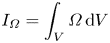 \begin{equation} I_{\varOmega} = \int_V \varOmega \,\mathrm{d} V \end{equation}
as well as the total enstrophy dissipation,
 \begin{equation} I_D = \int_V D \,\mathrm{d} V,\end{equation}
and the total enstrophy generation on the boundary,
 \begin{equation} I_F = \int_S F_{\varOmega} \,\mathrm{d} S,\end{equation}
under the L–H interpretation, in non-dimensional form. Here,  $V$ is a volume comprising the entire fluid, whereas
  $S$ is the surface of the sphere. After being generated by the initial rotation of the sphere, the total enstrophy decays due to enstrophy dissipation, approaching a constant value in the steady-state limit. In the steady-state flow, the generation and dissipation of enstrophy are zero under the L–H interpretation.

Figure 7. Time history of the total enstrophy ( $I_\varOmega$), enstrophy dissipation (
 $I_D$) and enstrophy generation (
 $I_F$) under (a) the L–H interpretation and (b) the L–P interpretation, presented in non-dimensional form.
Under the L–P definition, however, the boundary enstrophy flux is given by (2.24)
 \begin{equation} F_{\varOmega}' = \boldsymbol{ \omega} \boldsymbol{\cdot} \boldsymbol{ \sigma}' = \omega_\phi \frac{\partial{u_\phi}}{\partial{t}} - \nu \boldsymbol{ \omega} \boldsymbol{\cdot} (\boldsymbol{\nabla} \boldsymbol{ \omega}) \boldsymbol{\cdot} \boldsymbol{\hat{e}}_r, \end{equation}
which is non-zero for all  $\tau > 0$, and therefore enstrophy is continually created on the boundary by the viscous effect. In figure 7(b), we plot the time history of the total enstrophy (
 $I_\varOmega$), as well as the total enstrophy generation (
 $I_F'$) and dissipation (
 $I_D'$) under the L–P interpretation, in non-dimensional form. Note that the scale of the vertical axes in figure 7(a,b) differ by an order of magnitude. The total enstrophy,
  $I_\varOmega$, is the same in each plot; however,
  $I'_F$ and
  $I'_D$ are substantially larger than
  $I_F$ and
  $I_D$. Under the L–P interpretation, enstrophy is continually generated on the boundary, and the generation of enstrophy is balanced by an equivalent increase in the enstrophy dissipation when compared to the L–H interpretation, so that the total rate-of-change of enstrophy is equivalent between the two interpretations. Under the L–P interpretation, the steady-state flow is maintained by the continuous generation of enstrophy on the sphere, and continual destruction of enstrophy by viscous dissipation in the fluid interior. Importantly, the total enstrophy,
  $I_\varOmega$, does not depend on whether the L–H or L–P interpretations are used, and only the dynamical interpretation of the motion differs between the two definitions.
3.3. Inertial flow over a rotating sphere
We now consider the inertial flow over a rotating sphere. One of the main features of this flow is the formation of a counter rotating vortex pair due to a collision between the boundary layers from the upper and lower hemispheres, which has been examined in great detail by Calabretto et al. (Reference Calabretto, Levy, Denier and Mattner2015); Calabretto, Denier & Levy (Reference Calabretto, Denier and Levy2019). We have previously examined the generation of vorticity in this flow (Terrington et al. Reference Terrington, Hourigan and Thompson2021), and the numerical results presented in this section are obtained using the finite volume approach outlined in that work.
Figure 8 presents a colour plot of the dimensionless enstrophy, as well as the projection of vortex lines in the  $x$–
$x$– $z$ plane, for a selection of flow times. In addition, a transient animation is provided in supplementary movie 3. Initially, enstrophy is mostly located in the boundary layer. Rotation of the sphere results in a centrifugal effect, so that vorticity and enstrophy in the boundary layer are advected towards the equator. Vorticity and enstrophy from the upper and lower hemispheres interact at the equator, forming a counter-rotating vortex pair, as well as a radial jet flow. For further details on the boundary layer collision and jet formation, refer to Calabretto et al. (Reference Calabretto, Levy, Denier and Mattner2015, Reference Calabretto, Denier and Levy2019).

Figure 8. Colour plot indicating the non-dimensional enstrophy, overlaid with the projection of vortex lines in the  $x$–
$x$– $z$ plane, for the flow over a rotating sphere at
  $Re = 1000$, over a range of dimensionless flow times (
 $\tau = tW$).
Here, our focus is on the generation and dissipation of enstrophy, under the L–H and L–P interpretations. Under L–H, the boundary vorticity flux is given by (2.21)
 \begin{equation} \boldsymbol{ \sigma} = \frac{\partial{u_\phi}}{\partial{t}} \boldsymbol{\hat{e}}_\theta + \left[\frac{u_\phi^2}{R\tan\theta} - \frac{1}{\rho R}\frac{\partial{p}}{\partial{\theta}} \right] \boldsymbol{\hat{e}}_\phi. \end{equation}
As with the Stokes flow over a sphere, tangential vorticity is generated by the initial acceleration of the sphere. However, azimuthal vorticity is also continually generated on the boundary by tangential pressure gradients and the centrifugal acceleration. These terms can be interpreted as the inviscid relative acceleration, where, in the absence of viscous forces, boundary fluid elements would suffer a centrifugal acceleration towards the equator. The inviscid generation of vorticity also results in the creation of enstrophy, with a boundary enstrophy flux given by
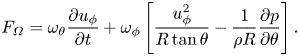 \begin{equation} F_{\varOmega} = \omega_\theta \frac{\partial{u_\phi}}{\partial{t}} + \omega_\phi \left[\frac{u_\phi^2}{R\tan\theta} - \frac{1}{\rho R}\frac{\partial{p}}{\partial{\theta}} \right]. \end{equation}
Under L–P, however, the boundary vorticity flux also includes the following viscous terms:
 \begin{equation} \boldsymbol{ \sigma}' = \boldsymbol{ \sigma} + \nu\left[\frac{\omega_\theta}{R} - \frac{1}{R}\frac{\partial{\omega_r}}{\partial{\theta}} \right] \boldsymbol{\hat{e}}_\theta + \nu\frac{\omega_\phi}{R} \boldsymbol{\hat{e}}_\phi - \nu \frac{\partial{\omega_r}}{\partial{r}} \boldsymbol{\hat{e}}_r, \end{equation}
and therefore vorticity creation is not an inviscid process. These terms also produce a corresponding viscous contribution to the L–P boundary enstrophy flux:
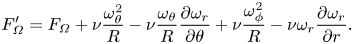 \begin{equation} F_{\varOmega}' = F_{\varOmega} + \nu\frac{\omega_\theta^2}{R} -\nu\frac{\omega_\theta}{R}\frac{\partial{\omega_r}}{\partial{\theta}} + \nu\frac{\omega_\phi^2}{R} - \nu \omega_r \frac{\partial{\omega_r}}{\partial{r}}. \end{equation}
 Figure 9(a) presents a time history of the total enstrophy  $I_\varOmega$. The initial rotation of the sphere generates an initially singular enstrophy, which is rapidly decayed by viscous dissipation. The total enstrophy then increases between
  $t/W = 5$ and
  $t/W = 10$, corresponding to the formation of the vortex pair, and remains approximately constant thereafter.
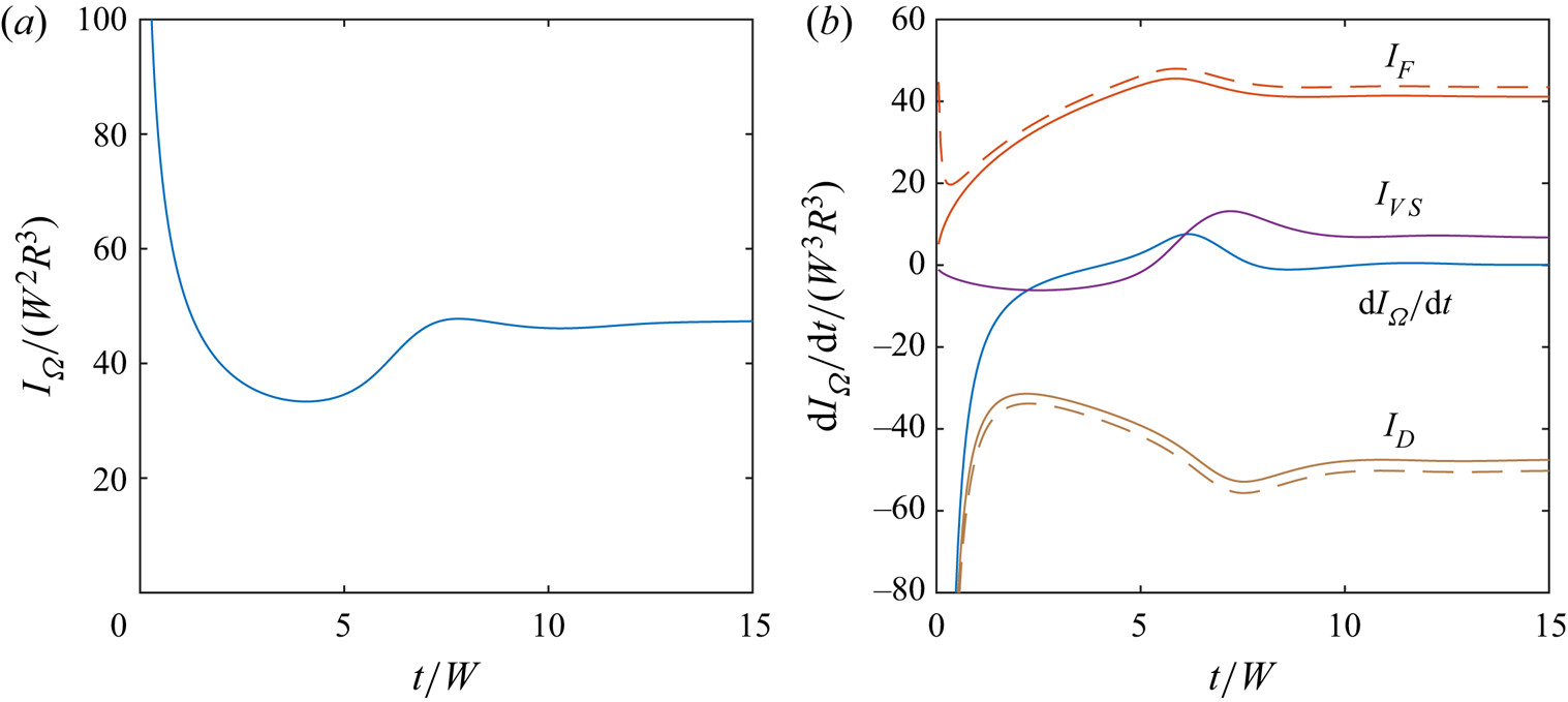
Figure 9. (a) Time history of the total enstrophy in the fluid. (b) Time history of the rate of change of enstrophy ( $\mathrm {d}I_\varOmega /\mathrm d t$), enstrophy dissipation (
 $I_D$), boundary enstrophy flux (
 $I_F$) and vortex stretching term (
 $I_{VS}$). Dashed lines are used for the L–P definitions, whereas solid lines are used for the L–H interpretation.
In figure 9(b), we plot the rate-of-change of total enstrophy, as well as the total enstrophy creation on the boundary ( $I_F$), enstrophy dissipation in the fluid interior (
 $I_D$) and enstrophy creation due to vortex stretching,
 \begin{equation} I_{VS} = \int_V \boldsymbol{ \omega} \boldsymbol{\cdot} \boldsymbol{\nabla} \boldsymbol{u} \boldsymbol{\cdot} \boldsymbol{ \omega} \,\mathrm{d} V. \end{equation}
Initially, the dissipation term dominates the boundary enstrophy flux and vortex stretching terms, producing the initial rapid decay of enstrophy. The vortex stretching and boundary enstrophy flux terms gradually increase, opposing the viscous dissipation of enstrophy. In particular, the formation of the vortex pair between  $t/W = 5$ and
  $t/W = 10$ is associated with a sharp increase in the enstrophy source due to vortex stretching, which produces an increase in the total enstrophy. Beyond
  $t/W = 10$, the total enstrophy creation by the boundary enstrophy flux and vortex stretching are approximately balanced by the enstrophy dissipation term, so that the total enstrophy remains approximately constant.
In figure 9, dashed lines indicate the dissipation and boundary flux terms under the L–P interpretation, whereas solid lines indicate the L–H interpretation. For most of the transient evolution, the two definitions give similar results, with only a small quantitative difference. The boundary enstrophy flux is slightly larger under the L–P interpretation, due to the additional viscous contribution, and this is balanced by an increased enstrophy dissipation compared with the L–H interpretation.
In figure 10, we plot the contributions to the boundary enstrophy flux from the pressure term ( $I_{F,p}$), the centrifugal acceleration (
 $I_{F,u}$) and the viscous term (
 $I_{F,\tau }$). Enstrophy creation is dominated by the centrifugal acceleration, which occurs under both the L–P and L–H interpretations. The viscous term, which only occurs under L–P, is small apart from the initial startup and, therefore, there are only small differences between the L–H and L–P interpretations for most of the transient evolution.
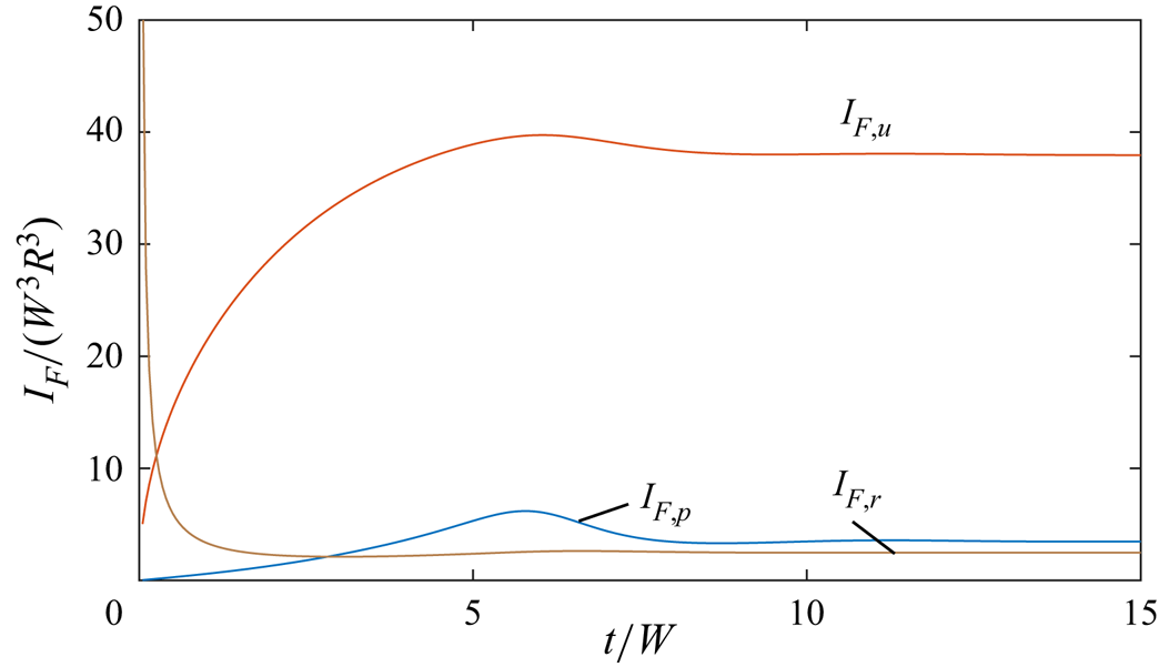
Figure 10. Contributions to the boundary enstrophy flux due to the centrifugal acceleration ( $I_{F,u}$), the tangential pressure gradients (
 $I_{F,p}$) and the viscous term (
 $I_{F,\tau }$).
The large differences between the L–H and L–P boundary enstrophy fluxes during the initial startup can be understood using the following argument. At  $t/W = 0^+$, the surface-normal vorticity is given by the no-slip boundary condition,
  $\omega _r = 2W \cos \theta$, whereas vorticity is zero in the fluid interior. Therefore, the vorticity gradient
  $\partial \omega _r/\partial r$ in (3.26) is singular following the initial rotation of the sphere. As the boundary layer develops, however, this term rapidly decreases, and is small for
  $t/W>1$.
In figure 11, we plot the spatial distribution of the enstrophy dissipation term at  $t/W = 12$ under (a) the L–P and (b) L–H interpretations. Visually, the distributions of enstrophy dissipation are nearly identical between the two definitions. Therefore, not only is the total enstrophy dissipation similar between the two interpretations, the structures associated with strong enstrophy dissipation, the boundary layer and the radial jet, are the same under both definitions. The differences between the two interpretations (
 $D - D'$) are plotted in figure 11(c), which confirms that while there are quantitative differences between the two interpretations, these differences are small.

Figure 11. Colour plot indicating the non-dimensional enstrophy dissipation under (a) the L–P and (b) the L–H interpretations, as well as (c) the difference between the two definitions, for the flow over a rotating sphere at  $Re = 1000$ and at
  $\tau = 12$. The projection of vortex lines in the
  $x$–
$x$– $z$ plane is also shown.
This example suggests that, while the L–H and L–P interpretations may be substantially different for highly viscous flows, for highly inertial flows the two interpretations give quite similar results. The quantity of enstrophy generated on the boundary, as well as the rate of dissipation in the fluid interior, are similar between the two interpretations. Moreover, the locations where enstrophy is generated, and the structures associated with strong enstrophy dissipation are also similar between the two interpretations. We have also examined a turbulent channel flow and the collision of symmetrical vortex rings (not presented for brevity), also finding only small differences between the L–H and L–P interpretations. Therefore, for a wide range of inertially dominated flows, one would not expect to find significant differences between the L–H and L–P interpretations.
We remark that even for inertially dominated flows, the L–H interpretation still offers several benefits for understanding the dynamics of vorticity. For example, the L–H interpretation has been used to provide an elegant description of the generation and conservation of vorticity in rotating and translating sphere flows (Terrington et al. Reference Terrington, Hourigan and Thompson2021), and for the interaction between a vortex ring and a free surface (Terrington et al. Reference Terrington, Hourigan and Thompson2022a). Even if the L–H and L–P interpretations of enstrophy dynamics are quantitatively similar for highly inertial flows, only the L–H interpretation of enstrophy dynamics is consistent with the L–H interpretation of vorticity dynamics.
This principle is clearly illustrated in the present example. Although the quantitative differences between the L–H and L–P boundary enstrophy fluxes are small, only the L–H interpretation is consistent with Morton's (Reference Morton1984) inviscid theory of vorticity creation. Therefore, the L–H interpretation offers a conceptually more elegant description of enstrophy creation, where enstrophy creation is interpreted as an inviscid process, due to the inviscid relative acceleration between the fluid and the boundary.
4. Conclusions
We have extended the L–P and L–H interpretations of vorticity dynamics to the dynamics of enstrophy. We have presented a consistent set of definitions for: the vorticity current, boundary vorticity flux, enstrophy current, boundary enstrophy flux and the enstrophy dissipation term, under each interpretation. Although the kinematic evolution of the vorticity and enstrophy fields are the same under each set of definitions, the dynamical interpretation of the motion generally differs. The local enstrophy creation rate on a boundary, as well as the local enstrophy dissipation in the fluid interior, may differ under each interpretation. Moreover, the total enstrophy generation on a solid body, as well as the total enstrophy creation in the fluid interior, may also differ between the two interpretations.
Importantly, the L–H interpretation of vorticity dynamics offers several advantages over the L–P interpretation, and the L–H interpretation of enstrophy dynamics developed in this work is consistent with the L–H interpretation of vorticity dynamics. For example, the L–H interpretation offers a conceptually simple interpretation of vorticity and enstrophy creation, where vorticity, and therefore enstrophy, creation is an inviscid process, driven by the relative acceleration between the fluid and the boundary. Under the L–P definitions, however, vorticity and enstrophy are also generated by a purely viscous mechanism.
Supplementary movies
Supplementary movies are available at https://doi.org/10.1017/jfm.2023.95.
Funding
This work was supported by the Australian Government through the Australian Research Council's Discovery Projects funding scheme (projects DP200100704 and DP210100990).
Declaration of interests
The authors report no conflict of interest.


 Open access