


1. Introduction and background
Turbulent boundary layers over rough and complex surfaces are ubiquitous and are of significant environmental and industrial interest. Surface roughness can induce significant frictional drag or pressure drop for flows in engineering settings, as summarised in the reviews by Flack & Schultz (Reference Flack and Schultz2010, Reference Flack and Schultz2014), and Chung et al. (Reference Chung, Hutchins, Schultz and Flack2021). Vegetation canopies are of great ecological importance to terrestrial and aquatic ecosystems, as reviewed by Finnigan (Reference Finnigan2000), Belcher, Harman & Finnigan (Reference Belcher, Harman and Finnigan2012), Nepf (Reference Nepf2012a,Reference Nepfb) and Brunet (Reference Brunet2020). Porous substrates are also present in a variety of settings (Wood, He & Apte Reference Wood, He and Apte2020), such as river beds (Vollmer et al. Reference Vollmer, de los Santos Ramos, Daebel and Kühn2002; Breugem, Boersma & Uittenbogaard Reference Breugem, Boersma and Uittenbogaard2006), heat exchangers (Lu, Stone & Ashby Reference Lu, Stone and Ashby1998; Dixon et al. Reference Dixon, Walls, Stanness, Nijemeisland and Stitt2012) and catalytic reactors (Lucci et al. Reference Lucci, Della Torre, Montenegro, Kaufmann and Eggenschwiler2017). In addition, engineered surfaces exposed to turbulent flows generally degrade and roughen due to erosion, fouling and cumulative damage (Wu & Christensen Reference Wu and Christensen2007). For these reasons, understanding the impact of complex surfaces on turbulence is essential for the modelling and control of practical flows, and to improve environmental and engineering practices.
The surface topology has a direct impact on the flow within the roughness sublayer, which generally extends up to 2–3 roughness heights  $h$, or spacings
  $s$, above the roughness crests, depending on the density regime (Jiménez Reference Jiménez2004; MacDonald et al. Reference MacDonald, Ooi, García-Mayoral, Hutchins and Chung2018; Brunet Reference Brunet2020). Above this height, it is accepted widely that the turbulence is essentially undisturbed and exhibits outer-layer similarity (Hama Reference Hama1954; Clauser Reference Clauser1956; Townsend Reference Townsend1976). The only effect is then a constant shift
  $\Delta U^+$ in the mean-velocity profile, while both the Kármán constant,
  $\kappa \approx 0.39$, and the wake region remain unaffected. Experimental evidence of outer-layer similarity was provided by Perry & Abell (Reference Perry and Abell1977) and Andreopoulos & Bradshaw (Reference Andreopoulos and Bradshaw1981), who reported smooth-wall-like mean-velocity profiles and turbulent statistics in the outer layer for flows over rough walls. The recovery of outer-layer similarity has also been observed in flows over a wide range of surface topologies, including two-dimensional ribs and grooves (Krogstad et al. Reference Krogstad, Andersson, Bakken and Ashrafian2005; Leonardi, Orlandi & Antonia Reference Leonardi, Orlandi and Antonia2007; MacDonald et al. Reference MacDonald, Ooi, García-Mayoral, Hutchins and Chung2018; Zhang, Huang & Xu Reference Zhang, Huang and Xu2020), sand grain (Flack, Schultz & Shapiro Reference Flack, Schultz and Shapiro2005; Connelly, Schultz & Flack Reference Connelly, Schultz and Flack2006; Amir & Castro Reference Amir and Castro2011; Flack & Schultz Reference Flack and Schultz2023), prismatic roughness (Castro Reference Castro2007; Yang et al. Reference Yang, Sadique, Mittal and Meneveau2016; Sadique et al. Reference Sadique, Yang, Meneveau and Mittal2017; Placidi & Ganapathisubramani Reference Placidi and Ganapathisubramani2018; Sharma & García-Mayoral Reference Sharma and García-Mayoral2020a; Xu et al. Reference Xu, Altland, Yang and Kunz2021) and practical rough surfaces (Shockling, Allen & Smits Reference Shockling, Allen and Smits2006; Allen et al. Reference Allen, Shockling, Kunkel and Smits2007; Wu & Christensen Reference Wu and Christensen2007). Jiménez (Reference Jiménez2004) argued that the recovery of outer-layer similarity relies on a large-scale separation
  $h/\delta <1/40$, where
  $\delta$ is the boundary layer thickness. Numerical studies of roughness and riblets have nevertheless observed outer-layer similarity for roughness with larger blockage ratios,
  $h/\delta =1/8$ for cubes in an open channel, and
  $h/\delta =1/7$ for sinusoidal roughness in a pipe (Leonardi & Castro Reference Leonardi and Castro2010; García-Mayoral & Jiménez Reference García-Mayoral and Jiménez2011; Chan et al. Reference Chan, MacDonald, Chung, Hutchins and Ooi2015; Abderrahaman-Elena, Fairhall & García-Mayoral Reference Abderrahaman-Elena, Fairhall and García-Mayoral2019; Sharma & García-Mayoral Reference Sharma and García-Mayoral2020a). As summarised in Chung et al. (Reference Chung, Hutchins, Schultz and Flack2021), the smooth-wall similarity in the wake region remains robust and holds even for intrusive roughness with
  $h/\delta \gtrsim 0.15$. In this obstacle regime (Jiménez Reference Jiménez2004), the protruding surface effect can completely disrupt similarity in the logarithmic layer, but the similarity is still recovered in the outer wake region (Flack & Schultz Reference Flack and Schultz2010, Reference Flack and Schultz2014).
Studies of wall-bounded turbulence have provided the tools for analysing and modelling rough-wall flows, with engineering models that treat roughness as a small perturbation to the smooth-wall flow (Flack et al. Reference Flack, Schultz and Shapiro2005; Flack, Schultz & Connelly Reference Flack, Schultz and Connelly2007). However, if the roughness-induced perturbation propagates into the outer layer, then the scaling based on smooth-wall similarity could result in inaccurate predictions for turbulent statistics and integral quantities. Understanding the extent of roughness effects and whether smooth-wall similarity holds true is therefore of great importance to various applications. Townsend (Reference Townsend1976) proposed the outer-layer similarity hypothesis, articulating that at a sufficiently high Reynolds number, essentially the turbulent eddies in the outer layer would be unaffected by the surface topology. The surface affects the flow only through providing the relevant scales, the wall shear stress  $\tau _w$, or the friction velocity
  $u_\tau =(\tau _w/\rho )^{1/2}$, and the characteristic length scale provided by the wall-normal distance to the wall,
  $y$. Townsend's hypothesis is essentially a dimensional argument stating that given
  $\delta ^+\gg 1$ and
  $h/\delta \ll 1$, surface effects are confined within the roughness sublayer, thus the only relevant scales for the flow above are
  $u_\tau$ and
  $y$, independent of the surface topology. Note that
  $u_\tau$ and
  $y$ are well defined for smooth-wall flows but may not be estimated easily for flows over rough and complex surfaces where the ‘wall’ is not obvious (Schultz & Flack Reference Schultz and Flack2007; Squire et al. Reference Squire, Morrill-Winter, Hutchins, Schultz, Klewicki and Marusic2016).
The canonical logarithmic form of the mean-velocity profile is
 \begin{equation} U^+= \frac{1}{\kappa}\log(y^++\Delta y^+)+A-\Delta U^+, \end{equation}
where  $\kappa$ is the Kármán constant, with
  $\kappa \approx 0.39$ if outer-layer similarity recovers,
  $A$ is the log-law intercept for a smooth-wall flow,
  $\Delta U^+$ is the velocity deficit caused by the drag induced by surface roughness,
  $y^+$ is the wall-normal distance, and
  $\Delta y^+$ is the zero-plane displacement that recovers outer-layer similarity for the mean-velocity profile
  $U^+$. Typically, the displacement
  $\Delta y^+$ is measured from the roughness tip or trough, and the zero-plane displacement height
  $y^+=-\Delta y^+$ corresponds to the height of the origin perceived by the outer-layer flow (Breugem et al. Reference Breugem, Boersma and Uittenbogaard2006; Manes, Poggi & Ridolfi Reference Manes, Poggi and Ridolfi2011).
Despite substantial evidence that supports Townsend's outer-layer similarity hypothesis in the presence of diverse surface topologies, some experimental studies cast doubt on its universal validity, reporting that the roughness effects can extend well into the outer layer (Krogstad, Antonia & Browne Reference Krogstad, Antonia and Browne1992; Krogstadt & Antonia Reference Krogstadt and Antonia1999; Tachie, Bergstrom & Balachandar Reference Tachie, Bergstrom and Balachandar2003; Bhaganagar, Kim & Coleman Reference Bhaganagar, Kim and Coleman2004). In these works, it was observed that the presence of roughness alters significantly the intensities of turbulent fluctuations, especially the wall-normal velocity fluctuations and Reynolds shear stress, and the mean-velocity profile even in the wake region. Additionally, recent experimental and numerical studies for turbulent flows over rough and complex surfaces, as summarised in table 1, have reported the existence of a logarithmic layer but with values for  $\kappa$, logarithmic slope, very different from the smooth-wall value
  $\kappa _s\approx 0.39$. Moreover, for studies with
  $\delta ^+\approx 1000\unicode{x2013}10\,000$ and
  $h/\delta \ll 1$, a decrease in
  $\kappa$ is still observed with an increase in Reynolds number for the same roughness, suggesting an in-depth modification of the flow by the substrates (Suga et al. Reference Suga, Matsumura, Ashitaka, Tominaga and Kaneda2010; Manes et al. Reference Manes, Poggi and Ridolfi2011; Fang et al. Reference Fang, Han, He and Dey2018; Okazaki et al. Reference Okazaki, Takase, Kuwata and Suga2021, Reference Okazaki, Takase, Kuwata and Suga2022). Some studies have observed that permeable roughness could lead to an approximately
  $50\,\%$ drop in
  $\kappa$, which is more substantial than that induced by the impermeable roughness with the same geometry, implying that permeability may enhance the extent and intensity of roughness effects (Okazaki et al. Reference Okazaki, Takase, Kuwata and Suga2021, Reference Okazaki, Takase, Kuwata and Suga2022; Esteban et al. Reference Esteban, Rodríguez-López, Ferreira and Ganapathisubramani2022; Karra et al. Reference Karra, Apte, He and Scheibe2022). Nevertheless, the prediction of
  $u_\tau$, which is of great importance for the assessment of outer-layer similarity, remains a challenge in experiments (Chung et al. Reference Chung, Hutchins, Schultz and Flack2021). Generally,
  $u_\tau$ is evaluated at the zero-plane displacement height, which is typically between the tip and trough of the obstacles, and
  $u_\tau$ is therefore not necessarily given by the total drag
  $\tau _w$ exerted on the surface. Depending on flow conditions and apparatus, uncertainties in
  $u_\tau$ and turbulent statistics are typically
  $\sim \pm 1\unicode{x2013}5\,\%$ (Schultz & Flack Reference Schultz and Flack2007, Reference Schultz and Flack2013; Squire et al. Reference Squire, Morrill-Winter, Hutchins, Schultz, Klewicki and Marusic2016).
Table 1. Studies that observe the modification of the logarithmic layer by the surface topology. The wall types are IPW (isotropic permeable wall), APW (anisotropic permeable wall) and IW (impermeable wall). Here,  $\delta ^+$,
  $\sqrt {K^+}$,
  $k_s^+$ and
  $\kappa$ are the reported friction Reynolds number (
 $\delta ^+=\delta u_\tau /\nu$, where
  $\delta$ is the boundary layer thickness or channel half-height,
  $u_\tau$ is the characteristic friction velocity and
  $\nu$ is the kinematic viscosity), permeability Reynolds number (
 $\sqrt {K^+}=\sqrt {K} u_\tau /\nu$, where
  $K$ is the permeability), roughness height (
 $k_s^+=k_s u_\tau /\nu$, where
  $k_s$ is the equivalent sand grain roughness height) and Kármán constant (
 $\kappa$). The abbreviations for the studies are B06 (Breugem et al. Reference Breugem, Boersma and Uittenbogaard2006), S10 (Suga et al. Reference Suga, Matsumura, Ashitaka, Tominaga and Kaneda2010), M11 (Manes et al. Reference Manes, Poggi and Ridolfi2011), R17 (Rosti & Brandt Reference Rosti and Brandt2017), K17 (Kuwata & Suga Reference Kuwata and Suga2017), S20 (Shen, Yuan & Phanikumar Reference Shen, Yuan and Phanikumar2020), K21 (Kazemifar et al. Reference Kazemifar, Blois, Aybar, Perez Calleja, Nerenberg, Sinha, Hardy, Best, Sambrook Smith and Christensen2021), K23 (Karra et al. Reference Karra, Apte, He and Scheibe2022), E22 (Endrikat et al. Reference Endrikat, Newton, Modesti, García-Mayoral, Hutchins and Chung2022), F18 (Fang et al. Reference Fang, Han, He and Dey2018), O21 (Okazaki et al. Reference Okazaki, Takase, Kuwata and Suga2021) and O22 (Okazaki et al. Reference Okazaki, Takase, Kuwata and Suga2022). Note that
  $\delta ^+$ denoted by
  $^*$ is estimated from
  $k_s^+$ and
  $k_s/\delta$ from S10. The values for
  $k_s^+$ and
  $\kappa$ from F18, denoted by
  $^*$, were provided for only some of their cases.

Recent studies carried out by Tuerke & Jiménez (Reference Tuerke and Jiménez2013) and Lozano-Durán & Bae (Reference Lozano-Durán and Bae2019) suggest that the scaling for wall turbulence is essentially local, and is set by the local mean shear and production rate of turbulent kinetic energy, with no explicit reference to the wall-normal distance  $y$. This implies that the traditional scaling based on
  $y$ and
  $u_\tau$ happens to hold because of the one-to-one correspondence between the latter and the local production and shear, but this correspondence does not need to hold necessarily for flows over non-smooth walls. As part of this work, we investigate, for flows that exhibit an apparent loss of outer-layer similarity, whether the local scale can still have correspondence to a friction velocity
  $u_\tau ^\star$ and a length scale
  $y_*$, where
  $y_*$ is the wall-normal distance to the zero-plane displacement height,
  $y_*=0$, but
  $u_\tau ^\star$ is not necessarily evaluated at
  $y_*=0$. In this work, superscript
  $\star$ denotes wall units defined by
  $\nu$ and
  $u_{\tau }^\star$ decoupled from
  $y_*=0$, and superscript
  $+$ denotes wall units defined by
  $\nu$ and
  $u_{\tau }^*$ evaluated at
  $y_*=0$. Subscript
  $*$ denotes outer units that are normalised by the bulk velocity
  $U_b$ and outer length scale
  $y_*$.
The diagnostic function of the mean-velocity profile in (1.1) is
 \begin{equation} \beta=y_*^+\,\frac{\partial U^+}{\partial y_*^+}, \end{equation}
where  $y_*=(y+\Delta y)/(\delta +\Delta y)$ is the wall-normal distance from the zero-plane displacement height at
  $y_*=0$, which would exhibit a plateau
  $\beta \approx 1/\kappa$ in the logarithmic layer if outer-layer similarity recovers (Mizuno & Jiménez Reference Mizuno and Jiménez2011; Luchini Reference Luchini2018). This diagnostic function is useful because deviations from the log-law profile are typically more apparent in
  $\beta$ in (1.2) than in
  $U^+$ in (1.1). Many previous studies therefore rely on the existence of this plateau in
  $\beta$ to determine the extent of the logarithmic layer and the inner scaling for flows over roughness (Breugem et al. Reference Breugem, Boersma and Uittenbogaard2006; Suga et al. Reference Suga, Matsumura, Ashitaka, Tominaga and Kaneda2010). Particularly, the linear relation between
  $U^+$ and
  $\log (y_*^+)$ in (1.1) is enforced by choosing a
  $\varDelta y$ that yields a plateau in
  $\beta (y_*^+)$. The inner velocity and length scales are then determined based on
  $u_\tau ^*$ evaluated at the reference height,
  $y_*=0$, yielding values for
  $\kappa$ that are not necessarily smooth-wall like, as listed in table 1. However, a logarithmic layer with a plateau in
  $\beta$ emerges only in flows at very high
  $Re_\tau$ (Lee & Moser Reference Lee and Moser2015; Hoyas et al. Reference Hoyas, Oberlack, Alcántara-Ávila, Kraheberger and Laux2022). More importantly, outer-layer similarity, by definition, refers to the similarity in not just the logarithmic layer but also the wake, the whole outer region. In the present work, we argue that for flows at all but the highest
  $Re_\tau$, neglecting smooth-wall similarity in the wake region while enforcing a plateau in the diagnostic function could result in spurious predictions of parameters, including
  $\Delta y$,
  $u_\tau ^*$ and
  $\kappa$, and friction-scaled turbulent statistics. In this study, we determine the zero-plane displacement
  $\Delta y$ by minimising the deviation compared to a smooth-wall flow of the diagnostic function not only in the logarithmic layer but also above. We assess the validity as a scaling velocity of the friction velocity
  $u_\tau ^*$ and
  $u_\tau ^\star$, both measured at the height of zero-plane displacement and set as an independent, free parameter. Additionally, we examine whether the value of
  $\kappa$ is modified by the type of surface or not. We probe the existence of outer-layer similarity in an extensive dataset of canopy flows. This choice is motivated by canopies being an instance of porous-like complex surfaces that are particularly obstructing and intrusive to the flow (Ghisalberti Reference Ghisalberti2009).
The paper is organised as follows. The numerical method and relevant canopy parameters are presented in § 2. Results, with particular emphasis on scaling for the outer-layer turbulence, are discussed in § 3. Finally, the conclusions are summarised in § 4.
2. Direct numerical simulations
We present results for a series of direct numerical simulations (DNS) of closed and open channels with canopies of rigid filaments covering the walls at moderate Reynolds numbers  $Re_\tau \approx 500\unicode{x2013}1000$. We note that these
  $Re_\tau$ are sufficiently high for convective effects to be dominant, such that the interpretation of the turbulent statistics in these canopy flows may be extrapolated to cases with higher
  $Re_\tau$ (Sharma & García-Mayoral Reference Sharma and García-Mayoral2020a). The streamwise, spanwise and wall-normal directions are
  $x$,
$x$,  $z$ and
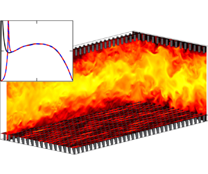
  $y$, respectively. A schematic of the numerical domain is portrayed in figure 1. The dimensions of the closed channels are
  $L_x \times L_z \times L_y=2{\rm \pi} \delta \times {\rm \pi}\delta \times 2(\delta +h)$, where
  $h$ is the canopy height, and
  $\delta =1$ is the distance between the channel centre and the canopy-tip planes. The canopy region is below
  $y=0$ for the bottom wall, and above
  $y=2\delta$ for the top wall. This domain size is large enough to reproduce the one-point statistics for the friction Reynolds numbers considered in this study, without imposing artificial constraints on the largest turbulent eddies (Lozano-Durán & Jiménez Reference Lozano-Durán and Jiménez2014).

Figure 1. Schematics of the numerical domains of (a) full-channel case C108 $_{550}$ and (b) open-channel case O400
 $_{550}$. An instantaneous realisation of the streamwise velocity is shown in the orthogonal planes.
We vary the canopy density by changing the spacing between elements, resulting in frontal densities  $\lambda _f\approx 0.01\unicode{x2013}2.04$, defined as the ratio between the frontal area of the obstacles and the total plan area. This covers a broad range from sparse to dense canopies based on the notional limit
  $\lambda _f\approx 0.1$ proposed by Nepf (Reference Nepf2012a). All canopies in the closed channel consist of collocated prismatic posts with thickness
  $\ell _x^+=\ell _z^+\approx 24$ and height
  $h^+\approx 110$. Relevant simulation parameters are listed in table 2. For the canopy simulations, letters C and O denote closed and open channels, and the number that follows denotes the approximate spacing,
  $s^+=L_x^+/n_x=L_z^+/n_z$, between the canopy elements, where
  $n_x$ and
  $n_z$ are the numbers of elements in the streamwise and spanwise directions, respectively. The number in the subscript is the approximate friction Reynolds number of the flow. Cases C216
 $_{900}$, C288
 $_{900}$ and C432
 $_{900}$ conducted at
  $Re_\tau \approx 900$ match the geometry parameters
  $s^+$,
  $l^+$ and
  $h^+$ of the sparse and intrusive cases C216
 $_{550}$, C288
 $_{550}$ and C432
 $_{550}$ in inner units, respectively. These cases at high Reynolds numbers are conducted to verify that outer-layer similarity can recover, even for flows over intrusive textures, provided that there is a large enough core flow unperturbed by the roughness. Cases C
 $_{550}$, C
 $_{600}$, C
 $_{900}$, O
 $_{550}$ and O
 $_{1000}$ are reference smooth-wall simulations.
Table 2. Simulation parameters:  $Re_\tau =\delta u_\tau /\nu$ is the friction Reynolds number based on
  $\nu$,
  $\delta$ and
  $u_\tau$ evaluated at the canopy tips;
  $\lambda _f$ is the frontal density;
  $N_x$ and
  $N_z$ are the numbers of canopy elements in the streamwise and spanwise directions, respectively;
  $h$ and
  $s$ are the canopy height and the spacing in the streamwise and spanwise directions;
  $\Delta x^+$ and
  $\Delta z^+$ are the streamwise and spanwise resolutions;
  $\Delta y_f^+$ and
  $\Delta y_t^+$ are the wall-normal resolutions at the floor and canopy tips. The wall-normal resolution is validated in the Appendix for reference. The O
 $_{550}$ and open-channel canopy cases are from Sharma & García-Mayoral (Reference Sharma and García-Mayoral2020a).

The DNS of sparse canopies,  $\lambda _f\approx 0.01$, from Sharma & García-Mayoral (Reference Sharma and García-Mayoral2020a), are included for the assessment of outer-layer similarity in open-channel flows. These channels are bounded by a bottom no-slip wall and a top free-slip surface at
  $y=\delta$, as shown in figure 1(b). Case O400
 $_{550}$ consists of prismatic posts with sides
  $\ell _x^+=\ell _z^+\approx 20$ and height
  $h^+\approx 110$. The canopy of O400
 $_{1000}$ matches the dimensions of O400
 $_{550}$ in inner units, with thickness
  $\ell _x^+=\ell _z^+\approx 20$ and height
  $h^+\approx 110$, while the canopy of C800
 $_{1000}$ matches the dimensions of O400
 $_{550}$ in outer units, with thickness
  $\ell _x/\delta =\ell _z/\delta \approx 0.04$ and height
  $h/\delta \approx 0.2$. The reference friction velocity
  $u_\tau$ in table 2 is calculated from the total shear stress at the canopy tips for the full-channel cases, and from the net drag for the open-channel cases. This is the reference friction velocity used in
  $Re_\tau =\delta u_\tau /\nu$ and in the other friction-scaled variables discussed in this section.
The DNS code implemented in this study is from Sharma & García-Mayoral (Reference Sharma and García-Mayoral2020a,Reference Sharma and García-Mayoralb) and has been validated in Sharma (Reference Sharma2020). It is summarised here for reference. The numerical method solves the three-dimensional incompressible Navier–Stokes equations
 \begin{gather} \frac{\partial\boldsymbol{u}}{\partial{t}} + \boldsymbol{u}\boldsymbol{\cdot}\boldsymbol{\nabla}\boldsymbol{u} ={-}\boldsymbol{\nabla}{p} + \frac{1}{Re}\,\nabla^2\boldsymbol{u}, \end{gather}
 \begin{gather}\boldsymbol{\nabla}\boldsymbol{\cdot}\boldsymbol{u} = 0, \end{gather}
where  $\boldsymbol {u}$ is the velocity vector
  $\langle u,w,v \rangle$ with components in the streamwise, spanwise and wall-normal directions, respectively,
  $p$ is the kinematic pressure, and
  $Re$ denotes the bulk Reynolds number
  $Re=U_b\delta /\nu$ based on
  $U_b$,
  $\delta$ and the kinematic viscosity
  $\nu$. No-slip and no-penetration boundary conditions are enforced at both walls. The canopy elements are resolved explicitly using a direct-forcing, immersed-boundary method (Iaccarino & Verzicco Reference Iaccarino and Verzicco2003; García-Mayoral & Jiménez Reference García-Mayoral and Jiménez2011). The numerical domain is periodic in the wall-parallel directions, which are discretised spectrally. A second-order central difference scheme on a staggered grid is used in the wall-normal direction to avoid the ‘chequerboard’ problem (Ferziger & Perić Reference Ferziger and Perić2002). The wall-normal grid is stretched with
  $\Delta y_{max}^+\approx 4.5$ at the channel centre for the closed-channel simulations. For the open-channel simulations,
  $\Delta y_{max}^+\approx 2.2$ when
  $Re_\tau \approx 550$, and
  $\Delta y_{max}^+\approx 5.3$ when
  $Re_\tau \approx 1000$. The
  $\Delta y_{min}^+$ value occurs at the floor or tips, wherever the mean shear is the highest;
  $\Delta y_{min}^+\approx 0.5\unicode{x2013}1$ is at the tips for the intermediate to dense canopies (
 $\lambda _f\gtrsim 0.1$), and
  $\Delta y_{min}^+\approx 0.3\unicode{x2013}0.8$ is at the floor for the sparse canopies (
 $\lambda _f\lesssim0.1$). The wall-normal grid resolutions are listed in table 2.
The typical wall-parallel resolutions are  $\Delta x^+\lesssim 8$ and
  $\Delta z^+\lesssim 4$ for the DNS of smooth-wall turbulent flows (Jiménez & Moin Reference Jiménez and Moin1991). However, for the filament canopies considered in this study, the element-induced eddies are typically of the order of or smaller than the element thickness (Poggi et al. Reference Poggi, Porporato, Ridolfi, Albertson and Katul2004). Therefore, the wall-parallel grids are smaller than
  $\ell _x^+$ and
  $\ell _z^+$ to resolve the eddies induced by the canopy elements, as presented in table 2. To resolve the turbulence within and above the roughness sublayer without inducing excess computational cost, the numerical domain is partitioned into blocks with different wall-parallel resolutions (García-Mayoral & Jiménez Reference García-Mayoral and Jiménez2011). The blocks that contain the roughness sublayer have a more refined resolution than the block encompassing the channel centre. In the fine blocks, the grid resolution resolves not just the turbulent scales but also the canopy geometry and element-induced eddies. The height of these blocks is chosen such that the small and rapid element-induced eddies diffuse naturally and damp out before reaching the coarse block at the channel centre, which has a standard
  $\Delta x^+\approx 8$ and
  $\Delta z^+\approx 4$ resolution. This is verified a posteriori by examining the spectral densities of turbulent fluctuations near the interface to ensure that any small-wavelength signal has already vanished.
The time advancement uses a fractional-step method with a three-substep Runge–Kutta scheme where pressure is corrected to enforce incompressibility (Le & Moin Reference Le and Moin1991; Perot Reference Perot1993):
 \begin{gather} \left[I-\Delta t\,\frac{\beta_k}{Re}\,L\right]\boldsymbol{u}^n_k = \boldsymbol{u}^n_{k-1}+\Delta t\left[\frac{\alpha_k}{Re}\,L\boldsymbol{u}^n_{k-1}-\gamma_kN\boldsymbol{u}^n_{k-1} -\zeta_kN\boldsymbol{u}^n_{k-2}-(\alpha_k+\beta_k)Gp^n_k\right], \end{gather}
 \begin{gather} DG\phi^n_k = \frac{1}{\Delta t\,(\alpha_k+\beta_k)}\,D\boldsymbol{u}^n_k, \end{gather}
 \begin{gather}\boldsymbol{u}^n_{k+1}=\boldsymbol{u}^n_k-\Delta t\,(\alpha_k+\beta_k)\,G\phi^n_k, \end{gather}
 \begin{gather}p^n_{k+1}=p^n_k+\phi^n_k, \end{gather}
where  $k = 1,2,3$ are the Runge–Kutta substeps (e.g.
  $u^0_0=u^0$,
  $u^0_3=u^1$),
  $\Delta t$ is the time step,
  $I$ is the identity matrix,
  $L$,
$L$,  $G$ and
  $D$ are the discretised Laplacian, gradient and divergence operators,
  $N$ is the advective term dealiased with the
  $2/3$-rule (Canuto et al. Reference Canuto, Hussaini, Quarteroni and Zang2012), and
  $\alpha _k$,
  $\beta _k$,
  $\gamma _k$ and
  $\zeta _k$ are the integration coefficients adapted from Le & Moin (Reference Le and Moin1991). The channel is driven by a constant mean pressure gradient, with the flow rate adjusted to obtain the targeted friction Reynolds number. Each simulation is run for at least 10 largest eddy turnover times,
  $\delta /u_\tau$, to wash out any initial transients. Once the flow reaches a statistically steady state, statistics are collected over another
  $20\delta /u_\tau$.
3. Results and discussion
In this section, we present and discuss the scaling for the outer-layer flow, aiming to show that for canopy flows that exhibit an apparent loss of outer-layer similarity, a modified outer-layer similarity can be recovered when using the appropriate velocity and length scales.
3.1. Depth of roughness layer
Before we set out to investigate outer-layer similarity, it is important to establish a lower bound for  $y$ from which it can be expected to hold. In the immediate vicinity of a complex surface, the flow cannot be expected to be universal, but will be specific to the particular surface topology. Outer-layer similarity should not be expected within the roughness sublayer, where turbulence is perturbed directly by the element-induced flow. Thus we first need to identify the height above which the direct effect of the texture, manifesting as a texture-coherent signature in the flow field, vanishes effectively. The height of the roughness sublayer, assumed here to be the height beyond which the element-induced flow vanishes, is generally a function of the element spacing or height, depending on the density regime (Jiménez Reference Jiménez2004; Brunet Reference Brunet2020). On the basis of canopy geometry and configuration, the frontal density
  $\lambda _f$ gives a notional measure of canopy density (Wooding, Bradley & Marshall Reference Wooding, Bradley and Marshall1973; Nepf Reference Nepf2012a). For conventional sparse canopies (
 $\lambda _f\lesssim 0.1$) with element spacing larger than height, the roughness sublayer thickness is typically a function of the canopy height (Poggi et al. Reference Poggi, Porporato, Ridolfi, Albertson and Katul2004; Flack et al. Reference Flack, Schultz and Connelly2007; Abderrahaman-Elena et al. Reference Abderrahaman-Elena, Fairhall and García-Mayoral2019; Sharma & García-Mayoral Reference Sharma and García-Mayoral2020a). However, for dense canopies (
 $\lambda _f\gtrsim 0.5$), the flow within the obstacles is ‘sheltered’ from the turbulent flow as the elements interact with turbulence only in the vicinity of the tips, thus the height of the roughness sublayer depends on the element spacing (MacDonald et al. Reference MacDonald, Ooi, García-Mayoral, Hutchins and Chung2018; Placidi & Ganapathisubramani Reference Placidi and Ganapathisubramani2018; Sharma & García-Mayoral Reference Sharma and García-Mayoral2020b). In the very dense limit, where the element spacings are vanishingly small, the eddies are essentially precluded from penetrating within the texture, and the overlying flow essentially perceives a smooth wall at the tips (Brunet Reference Brunet2020; Sharma & García-Mayoral Reference Sharma and García-Mayoral2020b).
To measure the extent of roughness effects, here we quantify the intensity of the element-induced flow using the standard triple decomposition (Reynolds & Hussain Reference Reynolds and Hussain1972)
 \begin{gather} \boldsymbol{u}(x,y,z,t) = \boldsymbol{U}(y)+\boldsymbol{u}'(x,y,z,t), \end{gather}
 \begin{gather}\boldsymbol{u}'(x,y,z,t)= \tilde{\boldsymbol{u}}(x,y,z)+\boldsymbol{u}''(x,y,z,t), \end{gather}
where  $\boldsymbol {u}$ is the full instantaneous velocity vector field
  $\langle u,w,v \rangle$,
  $\boldsymbol {U}$ is the mean-velocity profile, and
  $\boldsymbol {u}'$ is the full temporal and spatial turbulent fluctuation, decomposed into a time-averaged but spatially varying component
  $\tilde {\boldsymbol {u}}$ and the remaining time-varying fluctuation
  $\boldsymbol {u}''$. Here,
  $\boldsymbol {U}$ is the velocity averaged in time and in the wall-parallel directions, and
  $\tilde {\boldsymbol {u}}$, often termed the dispersive flow (Castro et al. Reference Castro, Kim, Stroh and Lim2021; Modesti et al. Reference Modesti, Endrikat, Hutchins and Chung2021), is obtained from the average of the flow in time only. Therefore, the root-mean-square (r.m.s.) of
  $\tilde {\boldsymbol {u}}$ at each height gives a measure of the intensity of the coherent spatial fluctuation induced by the canopy elements. Abderrahaman-Elena et al. (Reference Abderrahaman-Elena, Fairhall and García-Mayoral2019) argued that
  $\tilde {\boldsymbol {u}}$ does not contain the whole element-coherent signal, but it nevertheless gives a good measure of its intensity.
As shown in figure 2, the intensity of the element-induced fluctuations decays exponentially with  $y$ above the tips. A similar decaying pattern has been observed in flows over superhydrophobic surfaces (Seo, García-Mayoral & Mani Reference Seo, García-Mayoral and Mani2015), three-dimensional sinusoidal roughness (Chan et al. Reference Chan, MacDonald, Chung, Hutchins and Ooi2018), prismatic roughnesses (Abderrahaman-Elena et al. Reference Abderrahaman-Elena, Fairhall and García-Mayoral2019) and filament canopies (Sharma & García-Mayoral Reference Sharma and García-Mayoral2020b). The cause can be traced to the pressure in this region satisfying a Laplace equation with two components, one forced by the nonlinear terms of the overlying flow, which is essentially texture-incoherent, and the other forced by the effective boundary conditions at
  ${y=0}$, induced by the texture. The latter then takes the form
  $\sim {\rm e}^{-y/\lambda }$ for each excited wavelength, for which the first texture harmonic,
  $\lambda =s$, decays more slowly and dominates (Kamrin, Bazant & Stone Reference Kamrin, Bazant and Stone2010; Seo et al. Reference Seo, García-Mayoral and Mani2015). The velocities satisfy in turn their own corresponding Laplace equations, with additional source terms from this texture-induced pressure, leading to similar exponential decays. Figure 2 evidences this exponential decay with
  $y/s$, which is particularly clear for the pressure, as well as for the wall-normal velocity, and to a lesser extent for the tangential velocities, which is to be expected given their more intense source terms in their respective Laplace equations.

Figure 2. The r.m.s. velocity and pressure fluctuations of the element-induced, dispersive flow normalised by  $u_\tau$ evaluated at the canopy tips: (a,e,i,m) and (c,g,k,o) full-channel cases; (b,f,j,n) and (d,h,l,p) open-channel cases. The solid lines from blue to red are cases C36
 $_{550}$ to C432
 $_{550}$ in the first and third columns, and cases O400
 $_{550}$, O400
 $_{1000}$ and O800
 $_{1000}$ in the second and fourth columns; the dashed-dotted lines represent the cases at
  $Re_\tau\approx 900$ with the same canopy layouts as the solid lines of the same colour, i.e. cases C216
 $_{900}$, C288
 $_{900}$ and C432
 $_{900}$, corresponding to cases C216
 $_{550}$, C288
 $_{550}$ and C432
 $_{550}$. The square markers represent height
  $y=s$ for cases at
  $Re_\tau \approx 550$, and the triangle markers represent that for cases at
  $Re_\tau \approx 900\unicode{x2013}1000$.
For all canopies considered, the texture-coherent pressure and velocity fluctuations essentially vanish at approximately one canopy spacing above the tips, as depicted in figure 2. However, this implies that the sparse ( $\lambda _f\lesssim 0.1$) and tall (
 $h\approx 0.2\delta$) canopies, C216
 $_{550}$, C288
 $_{550}$, C432
 $_{550}$, O400
 $_{550}$ and O800
 $_{1000}$, are significantly more intrusive to the overlying flow compared to the other canopies with either intermediate to high density (
 $\lambda _f\gtrsim 0.1$) or small height (
 $h\approx 0.1\delta$), as their element-induced flows penetrate into the channel as far as
  $y\approx 0.5\delta$, or even beyond. This implies that the roughness sublayer of these intrusive canopies can extend well into the overlying flow and reach the channel centre. Sharma & García-Mayoral (Reference Sharma and García-Mayoral2020b) have reported a similar behaviour for the element-induced flow over dense canopies, for which the element-induced velocity fluctuations become negligible at one canopy spacing above the tips regardless of the canopy height. However, their element-induced flows caused a more profound modification of the background turbulence, which became smooth-wall-like only at heights
  $y/s>2-3$ above the tips. For the present flows, however, it will be demonstrated in §§ 3.3 and 3.4 that for the cases that exhibit it, outer-layer similarity recovers above a roughness sublayer that extends only to a height
  $y/s\approx 1$ above the tips.
3.2. Logarithmic velocity profiles over smooth and rough walls
In this subsection, we discuss and appraise the conventional methods used to assess the existence of a logarithmic layer, and find the zero-plane displacement height  $y_*=0$ that sets the velocity and length scales
  $u_\tau ^*$ and
  $y_*$ for turbulent flows over roughness. Generally, their values are determined by using the total drag (Jackson Reference Jackson1981; Raupach Reference Raupach1992; Cheng et al. Reference Cheng, Hayden, Robins and Castro2007; Leonardi & Castro Reference Leonardi and Castro2010; Squire et al. Reference Squire, Morrill-Winter, Hutchins, Schultz, Klewicki and Marusic2016), by fitting
  $U^+$ to be proportional to
  $\log (y_*^+)$ in the logarithmic layer (Clauser Reference Clauser1956; Flack & Schultz Reference Flack and Schultz2014), or by, equivalently, enforcing a plateau in
  $\beta$ (Breugem et al. Reference Breugem, Boersma and Uittenbogaard2006; Suga et al. Reference Suga, Matsumura, Ashitaka, Tominaga and Kaneda2010; Manes et al. Reference Manes, Poggi and Ridolfi2011).
In experiments, generally, friction velocity and zero-plane displacement height are estimated based on the total drag exerted on the surface, as summarised in Chung et al. (Reference Chung, Hutchins, Schultz and Flack2021). For small and sparsely distributed roughness, where the overlying flow penetrates all the way to the floor, this method generally yields  $u_\tau ^*$ and
  $\Delta y$ that recover outer-layer similarity (Flack et al. Reference Flack, Schultz and Shapiro2005; Wu & Christensen Reference Wu and Christensen2007; Schultz & Flack Reference Schultz and Flack2013). However, for dense and tall roughness, the total drag method could result in non-physical prediction for both
  $u_\tau ^*$ and
  $\Delta y$. The element-induced drag is significant for dense roughness, therefore the point of action of the total drag,
  $\Delta y=\int _h D(y)\,y\,{\rm d}y/\int _h D(y)\,{{\rm d}y}$ (Jackson Reference Jackson1981), is located at an intermediate point in the roughness sublayer. However, DNS of dense filament canopies have illustrated that the zero-plane displacement height approaches the tips as the overlying turbulence interacts only with the upper part of the obstacles and cannot perceive the floor (Brunet Reference Brunet2020; Sharma & García-Mayoral Reference Sharma and García-Mayoral2020b). In turn, for sparse canopies, the zero-plane displacement height approaches the floor, even when most of the drag is still exerted by the canopy elements (Sharma & García-Mayoral Reference Sharma and García-Mayoral2020a). Consequently, the total drag may not necessarily be relevant directly for the assessment of outer-layer similarity and the estimates of the zero-plane displacement
  $\Delta y$ and the friction velocity evaluated at
  $y_*=0$,
  $u_\tau ^*$.
Hama (Reference Hama1954) and Clauser (Reference Clauser1956) noted that generally, roughness leads to a downward but otherwise parallel shift  $\Delta U^+$ in the mean-velocity profile. It stems from this that
  $\Delta y$ and
  $u_\tau ^*$ can be obtained by matching the shape of the mean-velocity profile over roughness
  $U^+$ to
  $\log (y_*^+)$, assuming that the latter represents accurately the corresponding smooth-wall profile. This matching is usually done iteratively. Figures 3(e,f) illustrate how, for the flows over our canopies,
  $U^+$ can be made logarithmic by selecting a suitable value of
  $\Delta y$ and taking
  $u_\tau ^*$ based on the total shear stress at the zero-plane displacement height. However,
  $U^+$ is not exactly logarithmic even in the logarithmic layer of a smooth-wall flow, so matching
  $U^+$ to
  $\log (y_*^+)$ as in figures 3(e,f) is different from matching
  $U^+$ to the smooth-wall profile in the logarithmic layer as in figures 3(c,d). As an example,
  $\Delta y\approx 0.1\delta \unicode{x2013}0.15\delta =0.5h\unicode{x2013}0.75h$ enforces a logarithmic mean-velocity profile for case C144
 $_{550}$, but with a non-smooth-wall-like
  $\kappa _c$, as evidenced in figures 3(a,e). In addition, the mean-velocity profile above the logarithmic layer is different from a corresponding smooth-wall profile, suggesting a breakdown of outer-layer similarity, even though
  $U^+$ was made logarithmic. Alternatively, by imposing
  $\Delta y\approx 0.1\delta =0.5h$, we may recover a smooth-wall-like logarithmic layer, as depicted in figure 3(c), where
  $\kappa _c\approx \kappa _s\approx 0.39$. Nevertheless, the outer-wake region is still not smooth-wall-like, which would still break full outer-layer similarity. Moreover, for the intrusive cases C432
 $_{550}$ and O800
 $_{1000}$, where the near-wall turbulence is disrupted completely by the element-induced flow, the mean-velocity profile could still be enforced to take a logarithmic or smooth-wall-like shape within the ‘logarithmic layer’, as shown in figures 3(c–f). Nevertheless, the flow above this ‘logarithmic layer’ is never smooth-wall-like. In contrast, outer-layer similarity may still be achieved without recovering a complete smooth-wall-like logarithmic region, as illustrated for case O400
 $_{1000}$ in figures 3(b,d,f), where the lower part of the logarithmic region is perturbed by the canopy, but the flow above
  $y_*^+\approx 130$ is essentially smooth-wall-like when
  $\Delta y =0.1\delta$. The above suggests that outer-layer similarity cannot be recovered simply by artificially matching
  $U^+$ to
  $\log (y_*^+)$, or a smooth-wall profile, exclusively in the logarithmic layer. The matching should be for any height above the roughness sublayer.

Figure 3. Mean-velocity and velocity-deficit profiles for (a,c,e) cases C144 $_{550}$ (solid colour lines) and C432
 $_{550}$ (dashed colour lines), and (b,d,f) cases O400
 $_{1000}$ (solid colour lines) and O800
 $_{1000}$ (dashed colour lines). From blue to red, results are based on (a,c)
  $\Delta y=0$ to
  $0.25\delta$ and (b,d)
  $\Delta y=0.05\delta$ to
  $0.15\delta$; the black solid lines are reference smooth-wall profiles (a) C
 $_{550}$ and (b) O
 $_{1000}$; the black dashed lines are the smooth-wall log-law profile
  $1/\kappa \log (y^+)+A$; and the shaded area marks the logarithmic region for smooth-wall flows,
  $y^+=80$ to
  $y=0.3\delta$ for closed channels, and
  $y^+=80$ to
  $y=0.2\delta$ for open channels. The upper bound of the log region in open channels is lower than that in a closed channel because the free-slip surface induces a ‘cutoff’ to the wake region, which limits the extent of the logarithmic layer.
Within the logarithmic layer, enforcing  $U^+$ to be logarithmic, or smooth-wall-like, is essentially equivalent to enforcing
  $\beta$ to have a plateau, or a smooth-wall-like region. While the shapes of both
  $U^+(y_*^+)$ and
  $\beta (y_*^+)$ contain the same information,
  $\beta$ is more sensitive to deviations from the smooth-wall reference profile, and it portrays directly the value of
  $1/\kappa$ if it exhibits a plateau in the logarithmic layer. For these reasons, some recent studies rely on
  $\beta$ to predict
  $\Delta y$ and
  $u_\tau ^*$ (Mizuno & Jiménez Reference Mizuno and Jiménez2011; Kuwata & Suga Reference Kuwata and Suga2017; Okazaki et al. Reference Okazaki, Takase, Kuwata and Suga2021, Reference Okazaki, Takase, Kuwata and Suga2022). Breugem et al. (Reference Breugem, Boersma and Uittenbogaard2006) and Suga et al. (Reference Suga, Matsumura, Ashitaka, Tominaga and Kaneda2010) argued that the slope of
  $U^+$ versus
  $\log (y_*^+)$ must be constant within the logarithmic layer, and the profile of
  $(y+\Delta y)\,{\rm d}U/{{\rm d}y}$ should therefore exhibit a plateau with value
  $u_\tau ^*/\kappa$. It is worth mentioning that although the method and argument by Breugem et al. (Reference Breugem, Boersma and Uittenbogaard2006) and Suga et al. (Reference Suga, Matsumura, Ashitaka, Tominaga and Kaneda2010) have been adapted by some recent studies, these studies actually maximise the extent of the plateau in the entire flow, instead of just within the logarithmic layer (e.g. figure 5 in Breugem et al. Reference Breugem, Boersma and Uittenbogaard2006, figure 6 in Rosti & Brandt Reference Rosti and Brandt2017, and figure 8 in Shen et al. Reference Shen, Yuan and Phanikumar2020). However, let us illustrate using one of our present cases that there are instances when enforcing a plateau within the logarithmic layer or maximising the extent of the plateau may result in a breakdown of outer-layer similarity. Figure 4(a) shows the diagnostic function of case C36
 $_{550}$, which consists of closely packed elements. A plateau in
  $\beta$ emerges within the logarithmic layer when picking
  $\Delta y=0.05\delta =0.25h$, and the extent of this plateau maximises when picking
  $\Delta y=0.1\delta =0.5h$. The resulting Kármán constant
  $\kappa _c\approx 0.32$ or
  $0.29$, respectively, is much smaller than the smooth-wall value
  $\kappa _s\approx 0.39$, implying a significant modification of the outer-layer mean-velocity profile by the substrate. For dense canopies like C36
 $_{550}$, however, we would expect the overlying turbulent flow to ‘skim’ over the canopy tips, as the turbulent eddies are precluded from penetrating within and interacting with the full height of the canopy, to the point that the flow above the tips resembles a smooth-wall flow (Brunet Reference Brunet2020; Sharma & García-Mayoral Reference Sharma and García-Mayoral2020b). Figure 4(b) illustrates that the scaling based on
  $\Delta y=0$ produces a smooth-wall-like diagnostic function for case C36
 $_{550}$, suggesting that the overlying flow indeed perceives an origin in the vicinity of the canopy-tip plane. The underlying problem is that the emergence of a logarithmic layer relies on a large Reynolds number
  $\delta ^+$ such that the only available length scale in the overlap region,
  $\nu /u_\tau \ll y\ll \delta$, is the wall-normal distance
  $y$ (Townsend Reference Townsend1976). Within this overlap region, only a dimensionless constant
  $\kappa =u_\tau /(y\,\partial U/\partial y)$, can be constructed (Luchini Reference Luchini2017). However, if
  $\delta ^+$ is not sufficiently large, then
  $u_\tau /(y\,\partial U/\partial y)$ need not exhibit a flat plateau, as shown in figure 5. For smooth-wall flows, even
  $Re_\tau \approx 5000$ is not yet sufficient for the diagnostic function to exhibit a completely flat plateau, according to numerical evidence (Lee & Moser Reference Lee and Moser2015; Hoyas et al. Reference Hoyas, Oberlack, Alcántara-Ávila, Kraheberger and Laux2022). The local value of
  $\beta \approx 1/\kappa$ in the logarithmic layer exhibits a dependence on
  $y/\delta$, or
  $y^+/Re_\tau$, caused by the contamination from the wake above (Jiménez & Moser Reference Jiménez and Moser2007; Mizuno & Jiménez Reference Mizuno and Jiménez2011; Luchini Reference Luchini2018). As shown in figure 5, even for smooth-wall flows, so long as
  $Re_\tau \lesssim 5000$, enforcing a plateau in
  $\beta$ would overlook this dependence, and result in non-physical zero-plane displacements and values of
  $\kappa$ down to 0.3, as those listed in the figure. The above results for smooth walls suggest that artificially prescribing a plateau in
  $\beta$, while not enforcing the similarity in the wake region, could result in an apparent but false breakdown of outer-layer similarity and values for
  $\kappa$ that are consistently lower than the true smooth-wall value, as those listed in table 1. It is worth mentioning that the logarithmic layer of a smooth-wall channel is generally understood to span from
  $y^+\approx 80$ to
  $y/\delta \approx 0.3$. It is therefore not possible to define
  $\kappa$ meaningfully for flows at Reynolds numbers
  $\delta ^+\lesssim 300$, for which there is no significant range of
  $y$ in which a logarithmic layer can manifest. Note that some of the flows in table 1 fall in this low-
 $Re$ range.

Figure 4. (a) Diagnostic function and (b) defect-law velocity profile, scaled with  $y_*$ and
  $u_\tau ^*$ for case C36
 $_{550}$. Black solid line, reference smooth-wall profile C
 $_{550}$; blue, violet and red solid lines, canopy statistics based on
  $\Delta y=0$,
  $0.05\delta$ and
  $0.1\delta$, respectively; black, violet and red dashed lines, values of
  $1/\kappa$ for smooth-wall and canopy flow, where
  $\kappa _s\approx 0.39$ and
  $\kappa _c\approx 0.32$ and 0.28, respectively.

Figure 5. Diagnostic function for smooth-wall channel flows at  $Re_\tau$ increasing from blue to red:
  $Re_\tau \approx 1000$, 2000, 5000 and
  $10\,000$. The solid lines represent
  $y^+\,{\rm d}U^+/{{\rm d}y}^+$, with
  $\Delta y=0$; the dash-dotted lines in (a) represent
  $\beta$ with
  $\Delta y^+\approx 40$, 27, 13, 7, so that a plateau is enforced within the logarithmic layer as in Manes et al. (Reference Manes, Poggi and Ridolfi2011) and Okazaki et al. (Reference Okazaki, Takase, Kuwata and Suga2021, Reference Okazaki, Takase, Kuwata and Suga2022); the dash-dotted lines in (b) represent
  $\beta$ with
  $\Delta y^+\approx 80$, 139, 311, 1004, so that the extent of the plateau is maximised as in Breugem et al. (Reference Breugem, Boersma and Uittenbogaard2006), Suga et al. (Reference Suga, Matsumura, Ashitaka, Tominaga and Kaneda2010), Kuwata & Suga (Reference Kuwata and Suga2017), Rosti & Brandt (Reference Rosti and Brandt2017), Fang et al. (Reference Fang, Han, He and Dey2018), Shen et al. (Reference Shen, Yuan and Phanikumar2020), Kazemifar et al. (Reference Kazemifar, Blois, Aybar, Perez Calleja, Nerenberg, Sinha, Hardy, Best, Sambrook Smith and Christensen2021), Okazaki et al. (Reference Okazaki, Takase, Kuwata and Suga2021, Reference Okazaki, Takase, Kuwata and Suga2022) and Karra et al. (Reference Karra, Apte, He and Scheibe2022). Notice that Okazaki et al. (Reference Okazaki, Takase, Kuwata and Suga2021, Reference Okazaki, Takase, Kuwata and Suga2022) use both methods (see figures 5c and 5(a,b,d) in Okazaki et al. Reference Okazaki, Takase, Kuwata and Suga2021, and figures 12 and 21 in Okazaki et al. Reference Okazaki, Takase, Kuwata and Suga2022). With
  $Re_\tau$ increasing, the horizontal dotted lines correspond to
  $\kappa _c\approx (0.32,0.34,0.37,0.40)$ in (a) and
  $\kappa _c\approx (0.29,0.29,0.31,0.30)$ in (b), and the vertical lines represent the upper bound of the logarithmic layer,
  $y/\delta \approx 0.3$. The
  $Re_\tau \approx 1000, 5000$ data are from Lee & Moser (Reference Lee and Moser2015), the
  $Re_\tau \approx 2000$ data are from Hoyas & Jiménez (Reference Hoyas and Jiménez2006), and the
  $Re_\tau \approx 10\,000$ data are from Hoyas et al. (Reference Hoyas, Oberlack, Alcántara-Ávila, Kraheberger and Laux2022).
To address the above issues, we propose to obtain  $u_\tau ^*$ and
  $\Delta y$ by minimising the deviation between the smooth-wall and canopy diagnostic functions everywhere above the roughness sublayer, not just in the logarithmic layer. It will be demonstrated in §§ 3.3 and 3.4 that this method consistently recovers outer-layer similarity.
3.3. Sensitivity of canopy diagnostic function
Outer-layer similarity can be expected to appear only above the roughness sublayer, of height  $y_{r}$, above which the canopy diagnostic function
  $\beta _c$ should be smooth-wall-like. Because the extent of roughness effects can vary depending on the canopy density, as shown in figure 2,
  $y_{r}$ needs to be determined separately for each canopy (Jiménez Reference Jiménez2004; Brunet Reference Brunet2020). Care must be taken, because if part of the roughness sublayer is included in the region where outer-layer similarity is sought, then the values of
  $\Delta y$ and
  $u_\tau$ may be distorted. Therefore, the latter region needs to be sufficiently far away from the wall,
  $y>y_{r}$, such that all surface effects have vanished. We determine the values of
  $\Delta y$ and
  $u_\tau$ that recover a smooth-wall-like diagnostic function, or mean-velocity profile, as those that minimise the deviation between
  $\beta _s$ and
  $\beta _c$, the smooth-wall and canopy diagnostic functions, above
  $y_{r}$. By this method, we recover a smooth-wall-like
  $\beta _c$ in the outer layer, including both the logarithmic layer and the ‘wake’ region.
As an example, for case C144 $_{550}$, figure 6 portrays
  $\beta _c$ scaled with
  $y_*$ and
  $u_\tau ^\star$, the friction velocity decoupled from
  $y_*=0$, based on three tentative values of
  $y_{r}$. For
  $y_{r}=0.074\delta =0.37h=0.28s$,
  $\beta _c$ is not smooth-wall-like, even if the deviation between
  $\beta _c$ and
  $\beta _s$ above
  $y_{r}$ is minimised. This is because the flow at this
  $y_{r}$ is still perturbed directly by the canopy elements, as
  $y_{r}$ is too small compared to
  $s$, which provides an estimate of the roughness sublayer thickness, as evidenced in figure 2. In turn, adopting
  $y_{r}=0.274\delta =1.37h=1.04s$ overestimates the roughness sublayer thickness, as
  $\beta _c$ is already smooth-wall-like based on
  $y_{r}\gtrsim 0.174\delta =0.87h=0.66s$, implying that the height affected by the canopy in this case is lower than
  $y_r/s\approx 2\unicode{x2013}3$ reported in Abderrahaman-Elena et al. (Reference Abderrahaman-Elena, Fairhall and García-Mayoral2019) and Sharma & García-Mayoral (Reference Sharma and García-Mayoral2020b). For this canopy, we can conclude that outer-layer similarity is recovered when
  $y_{r}\approx 0.66s$, and beyond this limit,
  $\beta _c$ and
  $\Delta y$ are insensitive to the lower bound from which outer-layer similarity is enforced, as illustrated in figures 6 and 7(b). The r.m.s. deviation between
  $\beta _c$ and
  $\beta _s$ above
  $y_{r}$ is minimised if
  $y_{r}$ is sufficiently far away from the canopy, as shown in figure 7(a).

Figure 6. Diagnostic function of case C144 $_{550}$ scaled with
  $\Delta y$ and
  $u_\tau ^\star$, the friction velocity decoupled from
  $y_*=0$, that minimise the r.m.s. deviation from the smooth-wall profile above
  $y_{r}$. Black solid line, reference smooth-wall profile at
  $Re_\tau \approx 550$; blue, violet and red solid lines, canopy statistics based on blue dashed line
  $y_{r}=0.074\delta$, violet dashed line
  $y_{r}=0.174\delta$, and red dashed line
  $y_{r}=0.274\delta$, respectively.

Figure 7. (a) The r.m.s. deviation between  $\beta _s$ and
  $\beta _c$ above
  $y_{r}$ and (b) zero-plane displacement
  $\Delta y$, versus
  $y_{r}$ for case C144
 $_{550}$. The horizontal dashed lines mark once and twice the baseline error; and the thick black vertical markers denote the lower and upper bounds for
  $y_{r}$ above which outer-layer similarity recovers. The vertical dashed lines are as in figure 6.
In the above, we have let  $\kappa _c=\kappa _s$ and
  $u_\tau ^\star$ be independent of
  $\Delta y$, and we obtain the values of
  $\Delta y$ and
  $u_\tau ^\star$ for each
  $y_r$ by minimising the difference between
  $\beta _c$ and
  $\beta _s$ for any
  $y$ above
  $y_r$. However, if
  $y_r$ is not chosen carefully, then the corresponding
  $\Delta y$ and
  $u_\tau ^\star$ may not result in a smooth-wall-like
  $\beta _c$ above
  $y_r$, as illustrated in figure 6. Therefore, we need to identify an appropriate lower bound for
  $y_r$ to correctly assess outer-layer similarity, sufficiently far away from the wall for all surface effects to vanish. Starting at too low values, as
  $y_r$ increases, the r.m.s. deviation of
  $\beta$ in figure 7(a) decreases and eventually stabilises at a baseline-error level, which may be used to guide the selection of the lower bound of
  $y_r$. Here, we propose a lower bound of
  $y_{r}$ such that the r.m.s. error is twice the baseline error. Above this lower bound, the deviation between
  $\beta _c$ and
  $\beta _s$ is small, suggesting that
  $\beta _c$ scaled with
  $y_*$ and
  $u_\tau ^\star$ is essentially smooth-wall-like. On the other hand,
  $y_{r}$ should not be adopted excessively far above the surface, because outer-layer similarity cannot be examined properly on too small a portion of the flow. We propose an upper bound for
  $y_{r}$ that is
  $0.1\delta$ above the lower bound, as the r.m.s. of
  $\beta _c-\beta _s$ varies little beyond this.
Using the method that we propose,  $y_{r}$ results in
  $\Delta y$ and
  $u_\tau ^\star$ that consistently recover outer-layer similarity, with the resulting
  $\Delta y$ being insensitive to the particular choice of
  $y_r$ within the range proposed above, as evidenced by the flat region in figure 7(b). As shown in figure 7(a), the height above which outer-layer similarity recovers for case C144
 $_{550}$ is
  $y_{r}=(0.174\pm 0.05)\delta =(0.87\pm 0.25)h=(0.66\pm 0.19)s$. This is smaller than the typical roughness sublayer thickness, which extends up to
  $2h\unicode{x2013}3h$ above the tips (Jiménez Reference Jiménez2004; Brunet Reference Brunet2020). Nevertheless, figure 2 illustrates that the dominant length scale for the intensity of the texture-coherent flow is the element spacing, and essentially, these texture-coherent flows vanish at one spacing above the tips. For intermediate to dense cases with
  $\lambda \gtrsim 0.1$, where
  $s/h\lesssim 1$, we observe the recovery of outer-layer similarity for
  $y_r\approx s\lesssim h$. Additionally, because
  $y_{r}/\delta$ is smaller than the typical upper bound of a logarithmic layer,
  $y\approx 0.3\delta$, we expect the recovery of a smooth-wall-like logarithmic layer. Based on the confidence interval for
  $y_{r}$, we obtain the zero-plane displacement
  $\Delta y=(0.113\pm 0.005)\delta =(0.57\pm 0.03)h$, as shown in figure 7(b), indicating that the outer-layer flow perceives an origin
  $y_*=0$ at a depth roughly halfway between the floor and the canopy tips. However, the height of
  $u_{\tau }^\star$, corresponding to a smooth-wall-like
  $\kappa$, is
  $y_{u_{\tau }^\star }=(0.553\pm 0.036)\delta =(2.77\pm 0.18)h$, which is below the canopy floor (note that
  $y_{u_{\tau }^\star }$ is decoupled from
  $y_*=0$).
The fact that outer-layer similarity can be assessed only above a minimum height  $y_r$ implies that such similarity cannot be assessed for certain flows/substrates. In figures 8(c,d) and 9(c), we observe a breakdown of outer-layer similarity for the open-channel cases O400
 $_{550}$ (
 $y_{r}\geq 0.636\delta$) and O800
 $_{1000}$ (
 $y_{r}\geq 0.274\delta$). This is because these intrusive canopies perturb the overlying flow extensively, well into the region where a logarithmic layer would have been found otherwise. In contrast, for intermediate to dense cases, C36
 $_{550}$ to C144
 $_{550}$, C216
 $_{900}$ to C432
 $_{900}$, and O400
 $_{1000}$, which have less intrusive canopies, the canopy flow becomes smooth-wall-like no higher than
  $y_{r}=0.224\delta$, allowing for the recovery of a smooth-wall-like outer layer. The canopy diagnostic functions in figures 9(a,b) also show that whether outer-layer similarity recovers depends on the extent of the roughness layer, which is associated with
  $y_{r}$. In contrast, prescribing a constant slope for
  $U^+$ versus
  $\log (y_*)$, or enforcing a plateau in
  $\beta _c$, can result consistently in a breakdown of outer-layer similarity and a Kármán constant different from the smooth-wall one, as illustrated in figures 9(c,d).

Figure 8. Mean-velocity profiles of the canopy and smooth-wall flows: (a,c) full-channel cases with less intrusive canopies, C36 $_{550}$ to C144
 $_{550}$, and C216
 $_{900}$ to C432
 $_{900}$; (b,d) open-channel cases. The coloured solid and dash-dotted lines represent cases as in in figure 2. The black solid lines represent smooth-wall reference profiles at
  $Re_\tau \approx 900\unicode{x2013}1000$, and the black dashed lines represent smooth profiles at
  $Re_\tau \approx 550$. The square markers represent the lower bound of
  $y_r$ for cases at
  $Re_\tau \approx 550$, and the triangle markers represent that for cases at
  $Re_\tau \approx 900\unicode{x2013}1000$.

Figure 9. Diagnostic functions of the canopy and smooth-wall flows: (a,c) full-channel cases; (b,d) open-channel cases. Plots (a,b) enforce smooth-wall-like  $\beta _c$ above
  $y_{r}$; (b,d) enforce plateaus in
  $\beta _c$. The lines and markers are as in figure 8.
3.4. Universality or non-universality of the Kármán constant
In the above, the friction velocity  $u_\tau ^\star$ was not computed from the stress at the zero-plane displacement height
  $y_*=0$, and was instead set as an independent variable, such that
  $\beta _c$ was smooth-wall-like and
  $\kappa$ was universal,
  $\kappa _c=\kappa _s$. Alternatively, the friction velocity
  $u_\tau ^*$ could be computed from the stress at
  $y_*=0$, and
  $\kappa _c$ found by enforcing a match of the diagnostic function to that of a smooth-wall profile. In the logarithmic layer, (1.2) can be expressed as
 \begin{gather} y_*\,\frac{{\rm d}U}{{\rm d}y_*}\, \frac{\kappa_s}{u_\tau^\star}=\kappa_s\,\beta(y_*,u_\tau^\star)\approx1, \end{gather}
 \begin{gather}y_*\,\frac{{\rm d}U}{{\rm d}y_*}\,\frac{\kappa_c}{u_\tau^*}=\kappa_c\,\beta(y_*,u_\tau^*)\approx1, \end{gather}
from which we can observe that the group  $\kappa /u_\tau$ needs to have a certain value, but the mean-velocity profile does not provide information on whether this should be achieved by fixing
  $\kappa$ and finding
  $u_\tau$, or vice versa, or otherwise. As long as
  $\kappa _c/u_\tau ^* = \kappa _s/u_\tau ^\star$, the modified logarithmic profile in (3.4) is recovered. Figure 10(a) shows that whether
  $u_\tau ^\star$ or
  $\kappa _c\neq \kappa _s\approx 0.4$ is set as an independent parameter, the resulting mean-velocity profile or diagnostic function is still smooth-wall-like. In this subsection, we discuss the implications of fixing either
  $u_\tau$ or
  $\kappa$. While it is not possible to identify which option provides a complete outer-layer similarity by inspecting just the mean-velocity profile, other turbulent statistics collapse with the smooth-wall data when the friction velocity is evaluated at the zero-plane displacement height. As an example, the Reynolds shear stress profile in figure 10(b) collapses to smooth-wall data when scaled with
  $u_\tau ^*$, compared to
  $u_\tau ^\star$. If, alternatively, a universal
  $\kappa _c$ is enforced, the Reynolds shear stress would differ from smooth-wall values by a factor
  $(u_\tau ^*/u_\tau ^\star )^2$. The spectral density maps in figure 11 also show that outer-layer similarity is achieved with
  $u_\tau ^*$ obtained from the shear at the zero-plane displacement height
  $y_*=0$, and
  $\kappa _c$ having a non-smooth-wall value.

Figure 10. (a) Modified diagnostic function  $\kappa \beta$, and (b) Reynolds shear stress, of case C144
 $_{550}$. Black solid line, reference smooth-wall profiles at
  $Re_\tau \approx 550$; red dashed line, canopy profile scaled with
  $u_\tau ^\star$ and
  $y_*$; blue solid line, canopy profile scaled with
  $u_\tau ^*$ and
  $y_*$.

Figure 11. Pre-multiplied spectral energy densities for case C144 $_{550}$ (line contours) and reference smooth-wall case C
 $_{550}$ (filled contour) normalised by their respectively r.m.s. level at
  $y_*=0.3\delta$. Red dashed line, canopy statistics scaled with
  $u_\tau ^\star$ and
  $\nu$; blue solid line, canopy statistics scaled with
  $u_\tau ^*$ and
  $\nu$. The contours are at 0.01, 0.05 and 0.1 times the r.m.s. level.
For the cases with less intrusive canopies, C36 $_{550}$ to C144
 $_{550}$, C216
 $_{900}$ to C432
 $_{900}$, and O400
 $_{1000}$, the r.m.s. velocity fluctuations, Reynolds shear stress and pre-multiplied spectral energy densities scaled with
  $u_\tau ^*$ essentially collapse with their respective smooth-wall values above a height
  $y_*\approx 0.3\delta$, as shown in figures 12–14. This suggests that
  $u_\tau ^*$, and not
  $u_\tau ^\star$, is the velocity scale for the outer-layer turbulence. However, for the more intrusive cases, for example O800
 $_{1000}$, the roughness sublayer extends well into the overlying flow, which no longer exhibits a smooth-wall-like logarithmic layer, as evidenced by the footprint of the element-induced flow in figures 14(i–l). These intrusive textures cause a more in-depth modification of the outer-layer flow, and can lead to the breakdown of outer-layer similarity. Similar observations have been reported on large riblets and porous walls, where outer-layer similarity is limited if surface effects penetrate into a significant portion of
  $\delta$ (Breugem et al. Reference Breugem, Boersma and Uittenbogaard2006; Manes et al. Reference Manes, Poggi and Ridolfi2011; Endrikat et al. Reference Endrikat, Newton, Modesti, García-Mayoral, Hutchins and Chung2022).

Figure 12. The r.m.s. velocity fluctuations scaled with  $y_*$ and
  $u_\tau ^*$: (a,c,e) full-channel cases; (b,d,f) open-channel cases. Lines are as in figure 8.

Figure 13. Reynolds shear stress scaled with  $y_*$ and
  $u_\tau ^*$: (a) full-channel cases; (b) open-channel cases. The lines are as in figure 8.

Figure 14. Pre-multiplied spectral energy densities for canopy flow (line contours) and reference smooth-wall cases (filled contours) normalised by their respective r.m.s. level at  $y_*=0.3\delta$: (a–d) full-channel cases; (e–h) and (i–l) open-channel cases. The line colour scheme is as in figure 8. The contours are at 0.01, 0.05 and 0.1 times the mean-square fluctuation level.
By minimising the r.m.s. deviation of  $\beta _c$ from
  $\beta _s$, as discussed in §§ 3.3 and 3.4, we obtain the values of
  $\Delta y$ and
  $u_\tau ^*$ that provide the scales for the outer-layer turbulent flow. The trend of the zero-plane displacement in figure 15(a) suggests that the flows over dense canopies perceive an origin close to the tips, and that this origin becomes deeper as the canopy density decreases. In figure 15(b), the densest case has a smooth-wall-like Kármán constant,
  $\kappa _c\approx 0.4$, and the value of
  $\kappa _c$ decreases as the canopy density decreases. However, for the sparsest cases,
  $\kappa _c$ appears to tend back to its smooth-wall value. We note that the decreases in
  $\kappa _c$ for all canopies in this study never exceed
  $15\,\%$ of its smooth-wall value, which is significantly smaller than obtained by fitting
  $U^+$ to a
  $\log (y_*^+)$ profile as in Breugem et al. (Reference Breugem, Boersma and Uittenbogaard2006), Suga et al. (Reference Suga, Matsumura, Ashitaka, Tominaga and Kaneda2010), Rosti & Brandt (Reference Rosti and Brandt2017), Kuwata & Suga (Reference Kuwata and Suga2017), Kazemifar et al. (Reference Kazemifar, Blois, Aybar, Perez Calleja, Nerenberg, Sinha, Hardy, Best, Sambrook Smith and Christensen2021) and Okazaki et al. (Reference Okazaki, Takase, Kuwata and Suga2021, Reference Okazaki, Takase, Kuwata and Suga2022), where the values of
  $\kappa _c$ reported were as low as
  $\kappa _c\approx 0.2$.

Figure 15. (a) Ratio of zero-plane displacement depth to canopy height,  $-\Delta y/h$, and (b) Kármán constant,
  $\kappa _c$, versus canopy density
  $\lambda _f$, for all cases considered. Markers
  $\bigcirc$,
  $\ast$,
  $\times$ and
  $\triangle$ represent full-channel cases at
  $Re_\tau \approx 550$ and
  $Re_\tau \approx 900$, and open-channel cases at
  $Re_\tau \approx 550$ and
  $Re_\tau \approx 1000$, respectively. The colour scheme is as in figure 2. Transparent markers represent cases with substantial texture-induced coherent flows in the outer layer, and coloured markers represent cases with a smooth-wall-like outer layer. In (a), the black dashed line represents
  $\Delta y$ corresponding to zero-plane displacement height at the canopy tip (
 $-\Delta y/h=0$) and at the floor (
 $-\Delta y/h=-1$). In (b), the black dashed line represents
  $\kappa _s\approx 0.39$.
The present results for dense and sparse canopies are consistent with the results in Nepf (Reference Nepf2012a), Brunet (Reference Brunet2020) and Chung et al. (Reference Chung, Hutchins, Schultz and Flack2021), who summarised that for roughness in the dense or sparse regime, the zero-plane displacement height approaches the roughness crest or trough, respectively. For instance, for the dense canopy C36 $_{550}$,
  $\lambda _f\approx 2.04$, the smooth-wall-like overlying flow perceives an origin at the tips, and the Kármán constant has a smooth-wall value
  $\kappa _c\approx \kappa _s\approx 0.39$, as illustrated in figure 15. MacDonald et al. (Reference MacDonald, Chan, Chung, Hutchins and Ooi2016) and Sharma & García-Mayoral (Reference Sharma and García-Mayoral2020b) have also observed such skimming flow for closely-packed sinusoidal roughness and filament canopies, where
  $s^+\lesssim 3$. In particular, in the dense regime, where the spacing between elements is comparable to the viscous length scale
  $\nu /u_\tau$, essentially the overlying turbulence is precluded from penetrating the roughness, and the unmodified overlying flow is smooth-wall-like with a zero-plane displacement height at the tips.
Sparse canopies, where the ratio between element spacing and height is large, are generally more intrusive than the intermediate to dense canopies because the roughness sublayer can extend to  $y/s\approx 1$ into the channel, as discussed in § 3.1. For the sparse and tall canopies, C216
 $_{550}$, C288
 $_{550}$, C432
 $_{550}$, O400
 $_{550}$ and O800
 $_{1000}$, the surface effects penetrate deep into the overlying flow and can reach the channel centre, impeding the assessment of outer-layer similarity. For these substrates, outer-layer similarity could be assessed only at higher
  $Re_\tau$. This motivated us to conduct simulations C216
 $_{900}$, C288
 $_{900}$, C432
 $_{900}$, O400
 $_{1000}$, for which the canopies have similar dimensions to C216
 $_{550}$, C288
 $_{550}$, C432
 $_{550}$, O400
 $_{550}$, in inner units, but such that the unperturbed core flow is a larger portion of the channel. As illustrated in figure 15, the larger-
 $Re_\tau$ flows allow for a clearer assessment of outer-layer similarity, with zero-plane displacement height at the floor, and
  $\kappa _c\approx \kappa _s\approx 0.39$. Our observations are consistent with those in Poggi et al. (Reference Poggi, Porporato, Ridolfi, Albertson and Katul2004), Nepf et al. (Reference Nepf, Ghisalberti, White and Murphy2007) and Sharma & García-Mayoral (Reference Sharma and García-Mayoral2020a), where the flows over sparse canopies exhibit characteristics of smooth-wall flows, with reference wall at the canopy floor.
Flows over canopies with an intermediate density ( $\lambda _f\gtrsim 0.1$) perceive an origin between the tips and floor, as shown in figure 15(a). For these intermediate canopies, with
  $s/h\lesssim 1$, the overlying flow interacts mainly with the upper part of the obstacles, and turbulence does not penetrate all the way to the floor (Grimmond & Oke Reference Grimmond and Oke1999; Luhar, Rominger & Nepf Reference Luhar, Rominger and Nepf2008; MacDonald et al. Reference MacDonald, Ooi, García-Mayoral, Hutchins and Chung2018; Sharma & García-Mayoral Reference Sharma and García-Mayoral2020b). These intermediate-canopy flows exhibit values of the Kármán constant
  $\kappa _c\approx 0.34\unicode{x2013}0.36$, different from the smooth-wall value
  $\kappa _s\approx 0.39$, implying that the intermediate canopies disrupt the overlying flow more profoundly than both dense and sparse substrates. Nevertheless, other than for the change in
  $\kappa$, the turbulent statistics remain essentially smooth-wall-like in the logarithmic layer and above, as depicted in figures 8, 9 and 12–14. This suggests a modified outer-layer similarity, where
  $\kappa _c\neq 0.39$, but where otherwise the turbulence is outer-layer-similar to a smooth-wall flow. For
  $h\ll \delta$, we could expect that the flow far from the wall is not influenced by the details of the surface topology, as is the classical view of wall turbulence (Clauser Reference Clauser1956). Further work is required to study if the same canopies would also exhibit
  $\kappa _c\neq 0.39$ at larger
  $\delta /h$ ratios, say
  $\delta /h\approx 40$ as proposed by Jiménez (Reference Jiménez2004).
4. Conclusions
In the present work, we have assessed outer-layer similarity in flows over canopies ranging from sparse to dense ( $\lambda _f\approx 0.01\unicode{x2013}2.03$) at
  $Re_\tau \approx 550\unicode{x2013}1000$. We have discussed and appraised the conventional methods for the assessment of outer-layer similarity, showing that these methods could be inaccurate for flows over dense roughness and for flows at moderate
  $Re_\tau$.
To investigate outer-layer turbulence, we first determined the depth of the roughness sublayer, within which the turbulence is disrupted significantly by the element-induced flow. It was shown that the roughness sublayer for the present flows extends to a height equal to the element spacing. For the cases with tall ( $h\approx 0.2\delta$) and sparse (
 $\lambda _f\ll 0.1$) elements, C216
 $_{550}$, C288
 $_{550}$, C432
 $_{550}$, O400
 $_{550}$ and O800
 $_{1000}$, the element-induced flows penetrate effectively into the channel as far as
  $y\approx 0.5\delta$, or even above. As a result, these intrusive canopies leave only a small portion of core flow unperturbed, making the assessment of outer-layer similarity difficult. To verify whether outer-layer similarity can recover for these intrusive cases, simulations at higher
  $Re_\tau$, producing a larger unperturbed region, were required.
Conventionally, outer-layer similarity for a flow over roughness is recovered by imposing a zero-plane displacement and the corresponding friction velocity on the mean-velocity profile, such that the logarithmic layer is smooth-wall-like. We have discussed some caveats of conventional drag-based and mean-velocity-based methods used to determine these constants. For drag-based methods, and for densely packed roughness elements, the point of action of the total drag is located within the elements, while the overlying flow actually perceives an origin in the vicinity of the tips. For mean-velocity-based methods, we have shown that at moderate  $Re_\tau$, even smooth-wall flows do not exhibit a constant slope for
  $U^+$ versus
  $\log (y_*^+)$, or a plateau in
  $\beta$. Therefore, matching the shape of
  $U^+$ to
  $\log (y_*^+)$, or equivalently, enforcing a plateau in the diagnostic function
  $\beta$, may result in an artificial breakdown of outer-layer similarity and spurious predictions for the zero-plane displacement and the friction velocity at any but the highest
  $Re_\tau$ available in DNS literature.
To obtain the zero-plane displacement and friction velocity scale that recovers a smooth-wall-like diagnostic function, we minimise the deviation between the canopy and smooth-wall diagnostic function everywhere above the roughness sublayer, instead of in the logarithmic layer alone. By this method, we obtain a smooth-wall-like  $\beta$ not only in the logarithmic layer, but also in the wake region, enforcing outer-layer similarity in its full sense. We also explore the possibility of the zero-plane displacement and the friction velocity being set independently, but find that outer-layer similarity is recovered more consistently when they are coupled. For the dense canopies like C36
 $_{550}$, the unmodified overlying flow is smooth-wall-like with a zero-plane displacement height at the tips, and the Kármán constant has a smooth-wall value
  $\kappa _c\approx \kappa _s\approx 0.39$. This is the case because the skimming turbulence is precluded from penetrating into the obstacles, and perceives an origin at the tips. For sparse canopies (
 $\lambda _f\ll 0.1$), the higher-
 $Re_\tau$ cases, C216
 $_{900}$, C288
 $_{900}$, C432
 $_{900}$ and O400
 $_{1000}$, allow for the assessment of outer-layer similarity, with zero-plane displacement height at the floor, and
  $\kappa _c\approx \kappa _s\approx 0.39$. For intermediate canopies (
 $\lambda _f\gtrsim 0.1$), with
  $s/h\lesssim 1$, the overlying flow interacts mainly with the upper part of the obstacles, and turbulence does not penetrate all the way to the floor. These intermediate-canopy flows perceive a zero-plane displacement height between the tips and floor, and exhibit values of the Kármán constant
  $\kappa _c\approx 0.34\unicode{x2013}0.36$, different from the smooth-wall value
  $\kappa _s\approx 0.39$, implying that the intermediate canopies disrupt the overlying flow more profoundly than both dense and sparse substrates. Nevertheless, other than for the change in
  $\kappa$, the turbulent statistics remain essentially smooth-wall like in the logarithmic layer and above.
Acknowledgements
This work was partially supported by EPSRC grant EP/S013083/1. For the purpose of open access, the authors have applied a Creative Commons Attribution (CC BY) licence to any Author Accepted Manuscript version arising from this submission. Computational resources were provided by the ‘Cambridge Service for Data Driven Discovery’ operated by the University of Cambridge Research Computing Service and funded by EPSRC Tier-2 grant EP/P020259/1 (projects cs066 and cs155), and by the ‘ARCHER2’ system in the UK, funded by PRACE (project pr1u1702) and EPSRC (project e776). All research data supporting this publication are available directly within this publication.
Declaration of interests
The authors report no conflict of interest.
Appendix. Grid independence and validation
In this study, the no-slip condition within the canopy elements is enforced using the direct-forcing, immersed-boundary method (Iaccarino & Verzicco Reference Iaccarino and Verzicco2003) as implemented in García-Mayoral & Jiménez (Reference García-Mayoral and Jiménez2011) and modified by Sharma & García-Mayoral (Reference Sharma and García-Mayoral2020a,Reference Sharma and García-Mayoralb). This method applies a body force term to the right-hand side of (2.4) and drives the velocity at the immersed-boundary points to zero. The reader is referred to the works of Sharma & García-Mayoral (Reference Sharma and García-Mayoral2020b) and Sharma (Reference Sharma2020) for a detailed discussion on the accuracy of the immersed-boundary method implemented and wall-parallel resolution used. In the present study, the velocity within the rigid canopy elements is observed to be less than  $0.1u_\tau$, with
  $u_\tau$ evaluated at the canopy tips, for all the DNS conducted. As portrayed in figure 16, the velocity at the ‘solid’ points within the obstacles is significantly smaller than that at the surrounding ‘fluid’ points, illustrating that the immersed-boundary method resolves the canopy topology.

Figure 16. Instantaneous realisations of the (a) streamwise, (b) wall-normal and (c) spanwise velocities in a plane intersecting the canopy elements for case C54 $_{550}$, scaled with
  $u_\tau$ evaluated at the canopy tips. The darkest red and blue contours represent intensities of
  $\pm$1.0, respectively.

Figure 17. Wall-normal resolution, scaled with  $\nu$ and
  $u_\tau$ evaluated at the canopy tips, for case C108
 $_{550}$ for a fine resolution (black solid line), a standard resolution (red solid line) and a coarse resolution (blue solid line).
To analyse grid convergence, we have carried out three DNS for case C108 $_{550}$ with different wall-normal resolutions, as portrayed in figure 17. Compared to smooth-wall flows, where the maximum mean shear occurs at the wall,
  ${\rm d}U^+/{{\rm d} y}^+=1$, in our flows it occurs at the canopy-tip plane and is not as high, in the present case
  ${\rm d}U^+/{{\rm d}y}^+\approx 0.16$, peaking again at the floor at
  ${\rm d}U^+/{{\rm d}y}^+=0.1$. Since the local shear is the driver of turbulence, the wall-normal resolution required for the direct simulation of these flows is thus lower than for smooth-wall flows in terms of
  $\Delta y^+$, and can be adjusted following the local shear, as shown in figures 17 and 18(b). Consistent with this discussion, let us also note that the resolution at the floor in all of our simulations, for the case portrayed (C108
 $_{550}$),
  $\Delta y^+\approx 2$, is actually
  $\Delta y^+\approx 0.3$ when scaled with the local, dynamically relevant friction velocity proposed in Sharma & García-Mayoral (Reference Sharma and García-Mayoral2018, Reference Sharma and García-Mayoral2020b). Figure 18 portrays the results obtained for the resolution used in this paper, plus one finer and one coarser. All results collapse, evidencing grid convergence.

Figure 18. Turbulent statistics based on  $\nu$ and
  $u_\tau$ evaluated at the canopy tips for case C108
 $_{550}$. The colour scheme is as in figure 17.


 Open access