


1. Introduction
The past few decades have seen tremendous progress in modern medicine, especially in the ways drugs and treatments are administered. Targeted drug delivery, a class of methods to deliver medication to specific organs or tissues, is showing great promise for patient care. One form of targeted drug delivery consists of inserting the drug in a micro- or nano-particle, called a carrier (Samanta, Hosseini-Nassab & Zare Reference Samanta, Hosseini-Nassab and Zare2016; Kolosnjaj-Tabi et al. Reference Kolosnjaj-Tabi, Gibot, Fourquaux, Golzio and Rols2019; Wei et al. Reference Wei, Sung, Guo, Chen, Wang, Qiu, Zhang, Pang, Wang and Zhang2020; Chang et al. Reference Chang, Ma, Xu, Xie and Ju2021; Kemp & Kwon Reference Kemp and Kwon2021; Zhang, Liu & Zhang Reference Zhang, Liu and Zhang2021; Fabozzi et al. Reference Fabozzi, Della Sala, di Gennaro, Barretta, Longobardo, Solimando, Pagliuca and Borzacchiello2023) that is then absorbed by the patient orally or via an injection. By using these carriers, the drug is kept from interacting with and affecting any healthy cells, tissues and organs as it safely makes its way through the bloodstream, thus minimizing negative side effects to the whole physiological system. Two features must be considered for effective and efficient drug delivery using carriers: design and control. Design must account for various factors, including shape (Liu et al. Reference Liu, Tan, Thomas, Ou-Yang and Muzykantov2012; Nejati et al. Reference Nejati, Vadeghani, Khorshidi and Karkhaneh2020). Experimental and numerical studies have shown that under flow conditions and in the presence of red blood cells, non-spherical shapes (including ellipsoids) display a better margination rate (localization towards the blood vessel walls) compared with spherical particles. This enhanced rate is particularly important for the carrier's ability to adhere and ultimately cross biological barriers (Cooley et al. Reference Cooley, Strode, Hoore, Fedosov, Mitragotri and Gupta2018; Mitchell et al. Reference Mitchell, Billingsley, Haley, Wechsler, Peppas and Langer2021). Control on the other end relies in part on the use of micro-robots that mimic the propulsion of biological microorganisms (Wu et al. Reference Wu, Chen, Mukasa, Pak and Gao2020). The propulsion of microorganisms in unbounded fluids and media has attracted a tremendous amount of interest since the pioneering works of Taylor (Reference Taylor1951) and Lighthill (Reference Lighthill1952). Studies have since extended these seminal works to investigate the propulsion of microorganisms in unbounded non-Newtonian and heterogeneous media (Yu, Lauga & Hosoi Reference Yu, Lauga and Hosoi2006; Lauga Reference Lauga2007; Leshansky Reference Leshansky2009; Zhu et al. Reference Zhu, Do-Quang, Lauga and Brandt2011; Pak et al. Reference Pak, Zhu, Brandt and Lauga2012; Datt et al. Reference Datt, Zhu, Elfring and Pak2015; Chisholm et al. Reference Chisholm, Legendre, Lauga and Khair2016; Lauga Reference Lauga2016; Gómez et al. Reference Gómez, Godínez, Lauga and Zenit2017; Nganguia & Pak Reference Nganguia and Pak2018). However, the use of carriers to enhance targeted drug delivery (Lee & Yeo Reference Lee and Yeo2015; Wu et al. Reference Wu, Chen, Mukasa, Pak and Gao2020) or the development of nanotechnologies to manipulate cells in confined spaces (Raveshi et al. Reference Raveshi, Halim, Agnihotri, O'Bryan, Neild and Nosrati2021) have led to increasing interest in the motion of microorganisms enclosed in various interfaces (Mirbagheri & Fu Reference Mirbagheri and Fu2016; Reigh & Lauga Reference Reigh and Lauga2017; Reigh et al. Reference Reigh, Zhu, Gallaire and Lauga2017; Daddi-Moussa-Ider, Lowen & Gekle Reference Daddi-Moussa-Ider, Lowen and Gekle2018; Hoell et al. Reference Hoell, Lowen, Menzel and Daddi-Moussa-Ider2019; Nganguia et al. Reference Nganguia, Zhu, Palaniappan and Pak2020b). One way of investigating the effects of these interfaces on propulsion is by considering the locomotion inside a closed domain. To this end, systems consisting of motile organisms enclosed in droplets have been designed (Clausal-Tormos et al. Reference Clausal-Tormos2008; Wen et al. Reference Wen, Yu, Zhu, Jang and Qin2015; Ding et al. Reference Ding, Qiu, Solvas, Chiu, Nelson and DeMello2016; Raveshi et al. Reference Raveshi, Halim, Agnihotri, O'Bryan, Neild and Nosrati2021). Recent theoretical studies of such systems assumed physical interfaces with various properties (Reigh et al. Reference Reigh, Zhu, Gallaire and Lauga2017; Shaik, Vasani & Ardekani Reference Shaik, Vasani and Ardekani2018; Sprenger et al. Reference Sprenger, Shaik, Ardekani, Lisicki, Mathijssen, Guzman-Lastra, Lowen, Menzel and Daddi-Moussa-Ider2020; Kree, Ruckert & Zippelius Reference Kree, Ruckert and Zippelius2021; Kree & Zippelius Reference Kree and Zippelius2021; Marshall & Brady Reference Marshall and Brady2021). In Reigh et al. (Reference Reigh, Zhu, Gallaire and Lauga2017) the authors considered a squirmer inside a clean droplet and obtained analytical solutions for the squirmer and droplet speeds in a concentric configuration (the squirmer and droplet share the same centre). With this configuration, they showed that the squirmer always moves faster than the droplet. However, a co-swimming state (equal speeds between squirmer and droplet) can be achieved by considering radial modes in the surface velocity of the squirmer. The authors further analysed the stability of the co-swimming state numerically by considering various eccentric configurations. A surfactant-covered droplet has also been considered in place of a clean droplet (Shaik et al. Reference Shaik, Vasani and Ardekani2018). As in Reigh et al. (Reference Reigh, Zhu, Gallaire and Lauga2017), the authors of the study concluded that the squirmer propels faster than the droplet, yielding an unstable concentric configuration. The authors went on to show that various eccentric configurations, in which the squirmer and droplet no longer share the same centre of mass, led to a stable co-swimming state. These recent findings have provided important insights on locomotion inside a droplet. The studies showed that the system can be tuned to achieve specific stable, co-swimming configurations. However, the results are limited to spherical squirmers enclosed in droplets in homogeneous Newtonian fluids. In reality, microorganisms often encounter heterogeneous environments with networks of obstacles embedded into viscous fluid media. For instance, spermatozoa navigate through cervical mucus with a filamentous network (Rutllant, Lopez-Bejar & Lopez-Gatius Reference Rutllant, Lopez-Bejar and Lopez-Gatius2005); some spirochetes swim through highly complex and heterogeneous media and cross the blood-brain barrier to infect the brain (Radolf & Lukehart Reference Radolf and Lukehart2006; Wolgemuth Reference Wolgemuth2015); bacteria Helicobacter pylori can invade the epithelial cells by moving through the gastric mucus gel that protects the stomach (Celli et al. Reference Celli2009; Mirbagheri & Fu Reference Mirbagheri and Fu2016). The presence of a sparse network of stationary obstacles embedded in an incompressible Newtonian fluid can be modelled using the Brinkman equations (Brinkman Reference Brinkman1949) that include the additional hydrodynamic resistance due to the network of stationary obstacles. The Brinkman equations have been employed to address the effects of a viscous heterogeneous environment on locomotion performance (Leshansky Reference Leshansky2009; Jung Reference Jung2010; Leiderman & Olson Reference Leiderman and Olson2016). In addition to the viscous heterogeneous environment, it was found that the swimming speed can be enhanced for specific combinations of permeability and geometric parameters of the swimmer (Leiderman & Olson Reference Leiderman and Olson2016).
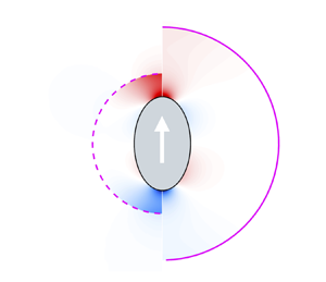
The squirmer model by Lighthill (Reference Lighthill1952) and Blake (Reference Blake1971) is adequate for spherically shaped ciliated organisms like Volvox (figure 1a). However, with a mean length-to-width aspect ratio of approximately 2, non-spherical ciliates are in fact more common (Lisicki et al. Reference Lisicki, Rodrigues, Goldstein and Lauga2019; Rodrigues, Lisicki & Lauga Reference Rodrigues, Lisicki and Lauga2021). Thus, a description of the squirmer that accounts for spheroidal geometry is needed to describe ciliated propulsion. Keller & Wu (Reference Keller and Wu1977) generalized the squirmer model to a prolate spheroidal body of arbitrary eccentricity that better represent organisms such as Paramecium and Tetrahymena (see figure 1b). The theoretical prediction of their spheroidal model found good agreement with experimental data of freely swimming and inert sedimenting Paramecium caudatum. Further generalization of the spheroidal model in Keller & Wu (Reference Keller and Wu1977) has been proposed to include higher modes of swimming to represent other types of swimmers (Ishimoto & Gaffney Reference Ishimoto and Gaffney2014; Theers et al. Reference Theers, Westphal, Gompper and Winkler2016; Pohnl, Popescu & Uspal Reference Pohnl, Popescu and Uspal2020), or to account for the effect of shape on squirming in non-Newtonian fluids (van Gogh et al. Reference van Gogh, Demir, Palaniappan and Pak2022). In addition to representing ciliates with spheroidal bodies, the spheroidal model serves as a first approximation to other non-spherical swimmers (e.g. Escherichia coli) to assess how geometrical shape affects swimming performance. We examine the dependence of caged microorganisms’ propulsion on (1) fluid heterogeneity (to model in vivo biological environments), and (2) squirmer and droplet shapes (for the control and design of micro-robots and drug carriers). The paper is organized as follows. First, we describe the setting and formulate the problem in § 2, which includes a discussion of the analytical (§ 2.2) and numerical (§ 2.3) methods employed in our study. We then derive the propulsion speeds of the spherical squirmer and droplets in § 3, validate our results against previous studies in § 3.1, and proceed to investigate the effects of the fluid resistance on the squirmer-droplet system (§ 3.2) and on its co-swimming state (§ 3.3). The second half of our study, § 4, investigates the effects of non-spherical squirmer and/or droplet shapes on propulsion in a homogeneous, Newtonian fluid. We analyse shape effects on the squirmer's individual (§ 4.1) and co-swimming (§ 4.2) speeds. The consideration of shapes reveal many interesting results that we further analyse by looking at the pressure and velocity profiles from the various configurations (§ 4.3). Finally, we summarize our findings in § 5 and discuss implications for current and future designs of drug delivery systems.

Figure 1. The squirmer represents ciliated microorganisms that can be approximated by (a) spherical shapes such as Volvox (adapted from https://www.britannica.com/science/Volvox/images-videos) or (b) spheroidal shapes such as Tetrahymena thermophila (reproduced from van Gogh et al. (Reference van Gogh, Demir, Palaniappan and Pak2022), which is distributed under the terms of the Creative Common CC BY license). (c) Geometric set-up and schematic of a squirmer in a Newtonian fluid pocket with viscosity  $\mu _1$ enclosed in a droplet in a heterogeneous medium with viscosity
  $\mu _2$. Both the squirmer and droplet are spheroids with semi-major and semi-minor axes
  $r_{maj,k}$ and
  $r_{min,k}$, respectively, where
  $k=s$ denotes the squirmer and
  $k=d$ denotes the droplet. (For spherically shaped squirmers and/or droplets,
  $r_{maj,k} = r_{min,k}$.) Here
  $\boldsymbol {n}$ and
  $\boldsymbol {s}$ denote the unit normal and tangent vectors to the spheroidal surfaces, respectively. The squirmer and droplet propel with speeds
  $U_S$ and
  $U_D$, respectively.
2. Formulation
We consider the propulsion of a spheroidal squirmer in an homogeneous Newtonian pocket encapsulated inside a spheroidal droplet in an heterogeneous medium, as illustrated in figure 1(c). The spheroidal squirmers and droplets have semi-major and semi-minor axes  $r_{maj,k}$ and
  $r_{min,k}$, respectively, where
  $k=s$ denotes the squirmer and
  $k=d$ the droplet. In the case of spherical squirmers and droplets (not displayed in figure 1c),
  $r_{maj,k} = r_{min,k}$. The fluid phases inside and outside the droplet have dynamic viscosities
  $\mu _1$ and
  $\mu _2$, respectively, and the squirmer and droplet propel with speeds
  $U_S$ and
  $U_D$, respectively. Following Reigh et al. (Reference Reigh, Zhu, Gallaire and Lauga2017), we assume that the droplet does not deform. This assumption is reasonable for spherically shaped droplets with sufficiently large surface tension, or for spheroidal droplets covered with shape-preserving surfactants and/or contaminants (Wall et al. Reference Wall, Harmsen, Pal, Zhang, Arianna, Lombardi, Drain and Kircher2017; Glushkova et al. Reference Glushkova, Cholakova, Biserova, Tsvetkova, Tcholakova and Denkov2023). Indeed, the contaminants give rise to surface viscosities that influence the surface dilatation and surface deformation of the droplet. The resulting forces act to stabilize the droplet's shape (Nganguia et al. Reference Nganguia, Das, Pak and Young2023).
The squirmer's surface velocity consists of radial and tangential modes. In the case of a spherical squirmer (Lighthill Reference Lighthill1952; Blake Reference Blake1971; Pedley Reference Pedley2016),
 \begin{equation} \tilde{\boldsymbol{u}}_{sq} = \sum^\infty_{n=0}A_nP_n\left(\cos\theta\right) \boldsymbol{e}_r + \sum^\infty_{n=1}B_nV_n\left(\cos\theta\right) \boldsymbol{e}_\theta, \end{equation}
where  $(\widetilde {\hspace {0.1in}})$ denotes a dimensional variable,
  $P_n(\cos \theta )$ are the Legendre polynomials,
  $V_n(\cos \theta )=-2P^1_n(\cos \theta )/[n(n+1)]$,
  $P^1_n(\cos \theta )$ are the associated Legendre polynomials of the first kind, and
  $A_n$ and
  $B_n$ are radial and tangential swimming modes, respectively. In the study of squirming microorganisms, it is customary to focus on the tangential modes. Furthermore, only the first two tangential modes (
 $B_n=0$ for
  $n>2$) are generally considered, since they help differentiate between various types of squirmers (such as neutral squirmers, pullers and pushers). However, we note that the interpretation and contribution of the tangential swimming modes
  $B_n$ to the propulsion speed and flow fields depend on the shape of the squirmer, as has been established by Pohnl et al. (Reference Pohnl, Popescu and Uspal2020). The propulsion speeds of a translating microorganism in an unbounded Newtonian fluid
  $U_N = 2B_1/3$ (Lighthill Reference Lighthill1952; Blake Reference Blake1971) and heterogeneous medium
  $U_B=6(1+\delta )B_1/(9+9\delta +\delta ^2)$ (Nganguia & Pak Reference Nganguia and Pak2018) depend only on the first actuation mode
  $B_1$. Since our focus is on changes in the propulsion speeds, we keep only the first modes
  $A_1$ and
  $B_1$ in the surface velocity (2.1).
2.1. The Stokes–Brinkman model
We extend the Stokes–Brinkman (N-B) model from our previous study (Nganguia et al. Reference Nganguia, Zheng, Chen, Pak and Zhu2020a) to account for the motion of the droplet. The Newtonian region ( $r_{maj,s}< r< r_{maj,d}$) is modelled as a purely viscous fluid governed by the incompressible Stokes equation
 \begin{equation} \tilde{\boldsymbol{\nabla}} \tilde{p}_1 + \mu_1\tilde{\boldsymbol{\nabla}}\times \left(\tilde{\boldsymbol{\nabla}}\times\tilde{\boldsymbol{u}}_1\right) = \boldsymbol{0}, \end{equation}
whereas the heterogeneous medium is governed by the Brinkman equations (Brinkman Reference Brinkman1949)
 \begin{equation} -\tilde{\boldsymbol{\nabla}} \tilde{p}_2 + \mu_2 \tilde{\nabla}^2\tilde{\boldsymbol{u}}_2 - \mu_2\omega^2\tilde{\boldsymbol{u}}_2 = \boldsymbol{0},\quad \tilde{\boldsymbol{\nabla}}\boldsymbol{\cdot}\tilde{\boldsymbol{u}}_2 = 0. \end{equation}
 To non-dimensionalize the problem, we scale the velocities using the first mode  $B_1$, lengths using the squirmer's semi-major axis
  $r_{maj,s}$ and pressure using
  $\mu _2B_1/r_{maj,s}$. In dimensionless form, the Stokes equation in the Newtonian domain (
 $1< r< b$) becomes
 \begin{equation} \boldsymbol{\nabla} p_1 + \lambda \boldsymbol{\nabla}\times\left(\boldsymbol{\nabla}\times\boldsymbol{u}_1\right) = \boldsymbol{0}, \end{equation}
where the ratio of semi-major axes  $b = r_{maj,d}/r_{maj,s}$ is the dimensionless droplet size that represents the size of the Newtonian domain, and
  $\lambda =\mu _1/\mu _2$ is the viscosity ratio. Similarly, the dimensionless Brinkman equations in the heterogeneous domain (
 $r>b$) is given by
 \begin{equation} -\boldsymbol{\nabla} p_2 + \nabla^2\boldsymbol{u}_2 - \delta^2\boldsymbol{u}_2 = \boldsymbol{0},\quad \boldsymbol{\nabla}\boldsymbol{\cdot}\boldsymbol{u}_2 = 0. \end{equation}
The governing equations are solved in the laboratory frame using the following boundary conditions. In the far field,
 \begin{equation} \boldsymbol{u}_2\left(r\rightarrow\infty\right) = \boldsymbol{0}, \end{equation}
while
 \begin{equation} \boldsymbol{u}_1\left(r=1\right) = \boldsymbol{U}_S + \boldsymbol{u}_{sq} \end{equation}
on the squirmer surface. The dimensionless surface velocity  $\boldsymbol {u}_{sq} = \alpha \cos \theta \boldsymbol {e}_r+ \sin \theta \boldsymbol {e}_\theta$, where
  $\alpha =A_1/B_1$. The boundary conditions on the droplet surface (
 $r = b$) are given by the continuity of normal velocities
 \begin{equation} u_1 = u_2 = U_D\cos\theta, \end{equation}
tangential velocities
 \begin{equation} v_1 = v_2 \end{equation}
and tangential components of surface force
 \begin{equation} \lambda \boldsymbol{n}\boldsymbol{\cdot}\boldsymbol{\mathsf{T}}_1\boldsymbol{\cdot}\boldsymbol{t} = \boldsymbol{n}\boldsymbol{\cdot}\boldsymbol{\mathsf{T}}_2\boldsymbol{\cdot}\boldsymbol{t}, \end{equation}
where  $\boldsymbol{\mathsf{T}}_j = -p_j\boldsymbol{\mathsf{I}} + \dot {{\varepsilon }}_j$,
  $\boldsymbol {t}$ and
  $\dot {{\varepsilon }}_j=\boldsymbol {\nabla }\boldsymbol {u}_j+(\boldsymbol {\nabla }\boldsymbol {u}_j)^{\rm T}$ denote the unit tangential vector and rate-of-strain tensor, respectively, and
  $j=1,2$.
2.2. Analytical solution
The Stokes velocity  $\boldsymbol {u}_1$ is obtained using Lamb's general solutions (Happel & Brenner Reference Happel and Brenner1973)
 $$\begin{gather} u_1 = \sum^\infty_{n=0}\left( O_nr^{n+1}+Q_nr^{n-1}+\frac{R_n}{r^n}+\frac{S_n}{r^{n+2}} \right) P_n\left(\cos\theta\right), \end{gather}$$
 $$\begin{gather}v_1 =\sum^\infty_{n=1}\left(-\frac{n+3}{2}O_nr^{n+1}-\frac{n+1}{2}Q_nr^{n-1}+ \frac{n-2}{2}\frac{R_n}{r^n}+\frac{n}{2}\frac{S_n}{r^{n+2}} \right) V_n\left(\cos\theta\right). \end{gather}$$
 The components  $u_2=\partial \psi _2/\partial \theta /r^2\sin \theta$ and
  $v_2=-\partial \psi _2/\partial r/r\sin \theta$ of the Brinkman velocity
  $\boldsymbol {u}_2$ are obtained from the streamfunction (Zlatanovski Reference Zlatanovski1999; Palaniappan Reference Palaniappan2014; Nganguia & Pak Reference Nganguia and Pak2018)
 \begin{equation} \psi_2 = \sin\theta \sum^\infty_{n=0} F_n(r) P^1_n\left(\cos\theta\right), \end{equation}
where
 \begin{equation} F_n(r) = T_nr^{-n}+Y_nr^{n+1}+\frac{\sqrt{r}}{\delta^2} [Z_n I_{n+{1}/{2}}(\delta r)+W_n K_{n+{1}/{2}}(\delta r)]. \end{equation}
Here,  $I_{n+{1}/{2}}$ and
  $K_{n+{1}/{2}}$ are modified Bessel functions of the first and second kind, respectively;
  $O_n, Q_n, R_n, S_n, T_n, Y_n, Z_n, W_n$ are coefficients determined by applying the boundary conditions. Note that in order to satisfy the boundary condition in the far field (2.6), the coefficients
  $Y_n=0$ and
  $Z_n=0$. Henceforth, we omit the index
  $n$ in the coefficients since we focus on a single-mode squirmer (
 $n=1$). The velocity in the Stokes domain becomes
 $$\begin{gather} u_1 = \left( Or^{2}+Q+\frac{R}{r}+\frac{S}{r^{3}} \right) \cos\theta , \end{gather}$$
 $$\begin{gather}v_1 = \left(-2Or^{2}-Q+\frac{1}{2}\frac{R}{r}+\frac{1}{2}\frac{S}{r^{3}} \right) \sin\theta, \end{gather}$$
and the corresponding velocity in the Brinkman domain is given by
 $$\begin{gather} u_2 = \left[ \frac{2T}{r^3}+ W \frac{{\rm e}^{-r\delta}\left(1+r\delta\right)}{\delta^{{7}/{2}} r^3}\right] \cos\theta, \end{gather}$$
 $$\begin{gather}v_2 = \left[ \frac{T}{r^3}+ W \frac{{\rm e}^{-r\delta}(1+r\delta+r^2\delta^2)}{\delta^{{7}/{2}} r^3} \right]\sin\theta . \end{gather}$$
Upon applying boundary conditions, we obtain the system of equations
 \begin{equation} \left(\begin{array}{@{}cccccc@{}} 1 & 1 & 1 & 1 & 0 & 0 \\ -2 & -1 & -\dfrac{1}{2} & \dfrac{1}{2} & 0 & 0 \\ -b^2 & -1 & -\dfrac{1}{b} & -\dfrac{1}{b^3} & \dfrac{2}{b^3} & s_1 \\ b^2 & 1 & \dfrac{1}{b} & \dfrac{1}{b^3} & 0 & 0 \\ 2b^2 & 1 & \dfrac{1}{2b} & -\dfrac{1}{2b^3} & \dfrac{1}{b^3} & s_2 \\ 3b & 0 & 0 & \dfrac{3}{b^4} & -\dfrac{6}{\lambda b^4} & s_3 \end{array}\right) \left[\begin{array}{@{}c@{}} O\\Q\\R\\S\\T\\W \end{array}\right] = \left[\begin{array}{@{}c@{}} \alpha+U_S\\1-U_S\\0\\U_D\\0\\0 \end{array}\right], \end{equation}
where
 \begin{equation} \left.\begin{gathered} s_1 = \frac{\sqrt{2 {\rm \pi}} {\rm e}^{-b \delta } \sqrt{b \delta } (b \delta +1)}{b^{7/2} \delta ^4}, \\ s_2 = \frac{\sqrt{\dfrac{{\rm \pi} }{2}} {\rm e}^{-b \delta } \sqrt{b \delta } (b^2 \delta ^2+b \delta +1)}{b^{7/2} \delta ^4}, \\ s_3 =-\frac{\sqrt{\dfrac{{\rm \pi} }{2}} {\rm e}^{-b \delta } \sqrt{b \delta } (b \delta (b \delta (b \delta +3)+6)+6)}{b^{9/2} \delta ^4 \lambda }, \end{gathered}\right\} \end{equation}
which yields the velocity field coefficients (see Appendix A). For both §§ 3 and 4, we first discuss the propulsion for purely tangential squirming modes ( $\alpha =0$), followed by an analysis of the co-swimming state (
 $\alpha \neq 0$).
2.3. Numerical simulations
The equations are solved numerically using the finite element method implemented in the COMSOL Multiphysics environment. To take advantage of the axial symmetry of the problem, an axisymmetric computational domain in the  $rz$ plane is used to simulate only half of the full flow domain. The equation describing the surface of the prolate spheroidal body reads
 \begin{equation} \frac{z^2}{r_{maj}^2} + \frac{r^2}{r_{min}^2} =1, \end{equation}
where  $r^2 = x^2+y^2$.
The squirmer and the droplet are modelled as half-prolate spheroids centred at the origin and whose major axes coincide with the axis of symmetry. The semi-major axis of the droplet,  $r_{maj,d}$, is scaled with
  $b>1$ such that
  $r_{maj,d}=b r_{maj,s}$ to model a range of droplet to squirmer size ratios. Semi-minor axes of both the squirmer and the droplet are calculated based on their respective eccentricities using the definition of eccentricity
  $e_k=c_k/r_{maj,k}$, where
  $c_k=(r_{maj,k}^2-r_{min,k}^2)^{{1}/{2}}$. Note that for a spherical shape,
  $e_k=0$.
A large computational domain of size  $500a_{sq} \times 500a_{sq}$ is employed to ensure negligible confinement effects. Here P1+P1 (first order for fluid velocity and first order for pressure) triangular mesh elements are used for the simulations, with local mesh refinement near the squirmer and inside the droplet domain to properly resolve the spatial variation of the flow field. The degree of freedom ranges from
  $1\times 10^5$ to
  $4\times 10^5$ for the simulations depending on
  $b$, which enlarges the finely meshed droplet domain as it gets larger and, therefore, increases the degree of freedom.
The unknown swimming velocity of the squirmer is obtained by solving the momentum and continuity equations simultaneously with the force-free swimming condition applied on the squirmer surface. Solving the fully coupled problem, we obtain the velocity and pressure fields. To find the droplet velocity, we evaluate the flow velocity at the droplet boundary. We used the parallel direct solver (PARDISO) for all simulations. It should be noted here that the numerical simulations compute the instantaneous velocities of the squirmer and the droplet while they are in a concentric configuration.
3. Effects of heterogeneity on propulsion
In this section we only consider the spherical squirmer and droplet. We substitute the velocity fields  $\boldsymbol {u}_j$ into the force-free conditions
 \begin{equation} \int_{\varGamma_1}\boldsymbol{\mathsf{T}}_1\boldsymbol{\cdot}\boldsymbol{n}\,{\rm d}\varGamma_1 = \boldsymbol{0},\quad \int_{\varGamma_2} \boldsymbol{\mathsf{T}}_2\boldsymbol{\cdot}\boldsymbol{n}\,{\rm d}\varGamma_2 = \boldsymbol{0}, \end{equation}
to determine the unknown swimming speeds of the squirmer  $U_S$ and droplet
  $U_D$. Here,
  $\varGamma _1$ and
  $\varGamma _2$ denote the squirmer and droplet interfaces, respectively. The swimming speed of the squirmer is given by
 \begin{align}
U_S &= \frac{1}{3\mathcal{B}}\left\{ (b-1)^2
(3+6b+4b^2+2b^3) ( 18+18b\delta + 3b^2\delta^2 +
b^3\delta^3)\right.\nonumber\\ &\left.\quad + 6
[-9 -9b\delta+15b^2+9b^5+(15b^3+9b^6)\delta +
(b^7-b^2)\delta^2 ] \lambda\right\},
\end{align}
\begin{align}
U_S &= \frac{1}{3\mathcal{B}}\left\{ (b-1)^2
(3+6b+4b^2+2b^3) ( 18+18b\delta + 3b^2\delta^2 +
b^3\delta^3)\right.\nonumber\\ &\left.\quad + 6
[-9 -9b\delta+15b^2+9b^5+(15b^3+9b^6)\delta +
(b^7-b^2)\delta^2 ] \lambda\right\},
\end{align}
and the swimming speed of the droplet is given by
 \begin{equation} U_D = \frac{30b^2\left(1+b\delta\right)\lambda}{\mathcal{B}}, \end{equation}
where
 \begin{equation} \mathcal{B} = (
b^5-1 ) ( 18+ 18b\delta+3b^2\delta^2+b^3\delta^3
) + (2+3b^5) ( 9+9b\delta+b^2\delta^2) \lambda. \end{equation}
\begin{equation} \mathcal{B} = (
b^5-1 ) ( 18+ 18b\delta+3b^2\delta^2+b^3\delta^3
) + (2+3b^5) ( 9+9b\delta+b^2\delta^2) \lambda. \end{equation}
In the presence of the dimensionless radial mode  $\alpha$, the squirmer speed becomes
 \begin{align} U_S &=
\frac{1}{\mathcal{B}_\alpha} \left\{ \frac{1}{\mathcal{B}}
[ 90 \lambda b ^2 (\alpha +1) (\delta b +1) [
5\delta (b ^6-b^3) +9 b ^5-5b^3+ \lambda (6 b^5+4)-4] ]\right.\nonumber\\ &\left.\quad - 2 [(\alpha -2) \delta b ^6+5 (\alpha +1)
\delta b ^3-3 b (2 \alpha \delta +\delta )+3 (\alpha -2)
(\lambda +1) b ^5 \right.\nonumber\\ &\quad \left. +3 (2
\alpha+1) (2 \lambda -3)+15 (\alpha +1) b ^2] \vphantom{\frac{1}{\mathcal{B}}}\right\}, \end{align}
\begin{align} U_S &=
\frac{1}{\mathcal{B}_\alpha} \left\{ \frac{1}{\mathcal{B}}
[ 90 \lambda b ^2 (\alpha +1) (\delta b +1) [
5\delta (b ^6-b^3) +9 b ^5-5b^3+ \lambda (6 b^5+4)-4] ]\right.\nonumber\\ &\left.\quad - 2 [(\alpha -2) \delta b ^6+5 (\alpha +1)
\delta b ^3-3 b (2 \alpha \delta +\delta )+3 (\alpha -2)
(\lambda +1) b ^5 \right.\nonumber\\ &\quad \left. +3 (2
\alpha+1) (2 \lambda -3)+15 (\alpha +1) b ^2] \vphantom{\frac{1}{\mathcal{B}}}\right\}, \end{align}
where
 \begin{equation} \mathcal{B}_\alpha = 6
[(b ^5-1)(\delta b +3)+\lambda (3 b
^5+2)], \end{equation}
\begin{equation} \mathcal{B}_\alpha = 6
[(b ^5-1)(\delta b +3)+\lambda (3 b
^5+2)], \end{equation}
and the droplet speed is given by
 \begin{equation} U_D = \frac{30 (\alpha +1) \lambda b ^2 (\delta b +1)}{\mathcal{B}}. \end{equation}
By setting (3.5) equal to (3.7) ( $U_{S} = U_{D}$), we obtain the ratio
  $\alpha _{SD}$ necessary for the squirmer and droplet to move at the same speeds,
 \begin{align}
\alpha_{SD} &= \frac{1}{\mathcal{B}_{SD} } [(b-1)^2(3+6b+4b^2+2b^3)
(18+18b\delta+3b^2\delta^2+b^3\delta^3) \nonumber\\ &\quad + 6(b^5-1)(9+9b\delta+b^2\delta^2)\lambda],
\end{align}
\begin{align}
\alpha_{SD} &= \frac{1}{\mathcal{B}_{SD} } [(b-1)^2(3+6b+4b^2+2b^3)
(18+18b\delta+3b^2\delta^2+b^3\delta^3) \nonumber\\ &\quad + 6(b^5-1)(9+9b\delta+b^2\delta^2)\lambda],
\end{align}
where
 \begin{align} \mathcal{B}_{SD} =
(b^5+5b^2-6)(18+18b\delta+3b^2\delta^2+b^3\delta^3) + 3(b^5+4)(9+9b\delta+b^2\delta^2)\lambda. \end{align}
\begin{align} \mathcal{B}_{SD} =
(b^5+5b^2-6)(18+18b\delta+3b^2\delta^2+b^3\delta^3) + 3(b^5+4)(9+9b\delta+b^2\delta^2)\lambda. \end{align}
Substituting  $\alpha _{SD}$ into (3.5) or (3.7) yields the co-swimming speed
 \begin{equation} U_{SD} = \frac{90b^2\left(1+b\delta\right)\lambda}{ \mathcal{B}_{SD} }. \end{equation}
3.1. Validation
We validate our analytical model and numerical implementation against the results in Reigh et al. (Reference Reigh, Zhu, Gallaire and Lauga2017), where the set-up consists of an encapsulated squirmer in a homogeneous Newtonian fluid ( $\delta =0$). In the limit of
  $\delta \rightarrow 0$, the propulsion speeds in (3.2) and (3.3) reduce to
 \begin{equation} U_S = \frac{2[3+5b^2(\lambda-1) - 3\lambda+b^5(2+3\lambda)]}{6(\lambda-1)+b^5(6+9\lambda)} \end{equation}
and
 \begin{equation} U_D = \frac{10b^2\lambda}{6(\lambda-1)+b^5(6+9\lambda)}. \end{equation}
These equations are identical to those in Reigh et al. (Reference Reigh, Zhu, Gallaire and Lauga2017, (19)) after letting  $\lambda = 1/\tilde {\lambda }$, where
  $\tilde {\lambda }$ is the viscosity ratio in their paper. Figure 2(a) shows the propulsion speed of the squirmer, while figure 2(b) shows the ratio of the droplet to squirmer speeds as a function of the droplet size
  $b$ with
  $\delta =10^{-3}$. The dashed curves denote the results using the purely viscous system in Reigh et al. (Reference Reigh, Zhu, Gallaire and Lauga2017), the solid curves are obtained from (3.11) and (3.12), and the symbols denote numerical simulations. Similarly, for the co-swimming state (figure 2c), the propulsion speed in (3.10) reduces to
 \begin{equation} U_{SD} = \frac{90\lambda b^2}{18(b^5+5b^2-6) + 27(b^5+4)\lambda}, \end{equation}
which, in the limit  $\delta \rightarrow 0$, is identical to the equation provided in (Reigh et al. Reference Reigh, Zhu, Gallaire and Lauga2017, (28)).

Figure 2. (a) Propulsion speed for the squirmer, (b) ratio of the droplet to squirmer speeds, and (c) propulsion speed for the co-swimming state ( $U_{SD} = U_S = U_D$) as a function of the droplet size
  $b$. In (a,c) the speeds are scaled by
  $U_N=2/3$, the propulsion speed of a squirmer in an unbounded Newtonian fluid. The dashed curves denote the results using the purely viscous system (see Reigh et al. (Reference Reigh, Zhu, Gallaire and Lauga2017), (10) and (11)), the solid curves are obtained from the N-B model ((3.11) and (3.12)), and the symbols denote numerical simulations. The fluid resistance
  $\delta =10^{-3}$ for the N-B model and the numerical simulations.
To further validate the numerical implementation of the Brinkman equations and the effects of the fluid resistance  $\delta$, we consider the flow decay. Figure 3 shows the magnitude of the velocity
  $\|\boldsymbol {u}_1+\boldsymbol {u}_2\|$ as a function of the distance from the squirmer's surface (
 $r=1$) with
  $b=1.025$ and
  $\lambda =10$. The velocity magnitude is plotted for
  $\theta =0$ (figure 3a) and
  $\theta ={\rm \pi} /2$ (figure 3b). The flow decays as
  $1/r^3$ in the far field (Nganguia & Pak Reference Nganguia and Pak2018), and we found excellent agreement between our analytical model (solid lines) and numerical simulations (symbols) for values of the fluid resistance
  $\delta =10^{-3},1,10$.

Figure 3. Velocity magnitude  $\|\boldsymbol {u}\| = \sqrt {u^2+v^2}$ as a function of the distance from the squirmer's surface for (a)
  $\theta =0$ and (b)
  $\theta {\rm \pi}/2$. In both panels,
  $b=1.025$ and
  $\lambda =10$. The solid curves are obtained from the N-B model and the symbols denote numerical simulations.
3.2. Effects of fluid resistance on the propulsion speed of the squirmer ( $\alpha =0$)

We now investigate the effects of the fluid resistance  $\delta$ on the propulsion speed of the squirmer. We focus on the squirmer since our results show that the squirmer's speed exhibits the most interesting variations. As the heterogeneous medium becomes more resistant to fluid motion (
 $\delta \rightarrow \infty$), the droplet's speed is completely suppressed (refer to Appendix B) while the squirmer continues propelling. This configuration is akin to restricting motile organisms in a static droplet to, for instance, investigate the dynamics of organism-surface interactions (Raveshi et al. Reference Raveshi, Halim, Agnihotri, O'Bryan, Neild and Nosrati2021). Also note that throughout this section, and unless otherwise noted, we compare the squirmer speed to that of a squirmer in an unbounded Newtonian fluid.
Figure 4 shows the propulsion speed scaled with  $U_N$ as a function of the fluid resistance
  $\delta$. Taken together, for all values of the viscosity contrast and across the range of fluid resistance, the squirmer is always able to move in its enclosure. Moreover, we note a non-trivial dynamics that depends on the viscosity ratio
  $\lambda$ and droplet size
  $b$. Figure 4(a) shows the speed for
  $\lambda =0.1$. In this case, the squirmer always moves slower than its unbounded counterpart. However, speed enhancement can be achieved relative to the droplet size. Comparing the curves in the range
  $\delta \lessapprox 1$, we observe that the speed is non-monotonic: as
  $b$ increases, the squirmer's speed first decreases before increasing after reaching a minimum. On the other end when
  $\delta >1$, the speed monotonically increases with a larger droplet size. The increase in the speed is not unexpected: as
  $b\rightarrow \infty$, the problem becomes identical to a squirmer in an unbounded Newtonian fluid.

Figure 4. Propulsion speed for the squirmer as a function of fluid resistance  $\delta$. In all panels, the speed is scaled by
  $U_N=2/3$, the propulsion speed of a squirmer in an unbounded domain in a Newtonian fluid. The solid curves are obtained from (3.2).
When  $\lambda =1$ (figure 4b), the squirmer speed is much the same as that experienced by a squirmer in a Newtonian pocket in a heterogeneous medium (Nganguia & Pak Reference Nganguia and Pak2018). Up to
  $\delta \approx 1$, the squirmer swims at the same speed experienced by a squirmer in an unbounded Newtonian fluid. The speed then decreases monotonically to a non-zero value. The magnitude of the speed as
  $\delta \rightarrow \infty$ is determined by the droplet size. Here, as in the case of a lower viscosity ratio, increasing
  $b$ has the effect of raising the squirmer's speed. For
  $\lambda =10$ and fluid resistance up to
  $\delta \approx 1$ (for
  $b=1.025$) or
  $\delta \approx 7$ (for
  $b\geq 1.5$), the squirmer always moves faster compared with a squirmer in an unbounded Newtonian fluid (as illustrated in figure 4c). Similarly to the case with a lower viscosity ratio, the speed varies non-monotonically with the droplet size. This time, as
  $b$ increases, the squirmer's speed reaches a maximum speed
  $U_S/U_N\approx 1.2$ (
 $b=1.5$). For larger values of the fluid resistance, the speeds asymptote to non-zero values, meaning the squirmer is always able to move albeit at a slower speed than that of a squirmer in an unbounded Newtonian fluid. For targeted drug delivery, it is advantageous that the squirmer and droplet move at the same speed as much as possible. A sufficient condition to attain this state is to account for the first radial swimming modes
  $A_1$ (Reigh et al. Reference Reigh, Zhu, Gallaire and Lauga2017) in the squirmer's surface velocity
  $\boldsymbol {u}_{sq}$ (2.1). Since the droplet propels in a heterogenous medium, one may ponder, naturally: How do the radial swimming mode and the co-swimming speed depend on the fluid resistance?
3.3. Dependence of the co-swimming variables on the fluid resistance ($\alpha \neq 0$)

To answer the previous question, we must analyse the dependence of the co-swimming mode ratio  $\alpha _{SD}$ (3.8) on the fluid resistance
  $\delta$. This dependence is illustrated in figure 5 for viscosity ratios
  $\lambda =0.1$ (a),
  $\lambda =1$ (c) and
  $\lambda =10$ (e). In all three panels,
  $\alpha _{SD}$ reveals two distinct regions of near-constant values: one at low fluid resistance and another at high fluid resistance. A transition region
  $\varDelta$ stretches across the interval
  $\delta \in [1,100]$. We observe that
  $\alpha _{SD}$ is larger for low
  $\delta$ compared with the smaller values at large
  $\delta$. The magnitude of the transition phase shows a non-monotonic dependence on the droplet size
  $b$: the difference between
  $\alpha _{SD}$ at small and large
  $\delta$ is such that it first increases with
  $b$ up to
  $\approx 1.5$, then asymptote to a non-zero lower value. These changes are more clearly observed at a high viscosity contrast (figure 5e). Physically, we can deduce that the radial mode is less effective at large fluid resistance. The co-swimming speed
  $U_{SD}$ is shown in figure 5(b,d,f). Taken together, they show that the squirmer-droplet system is fastest at low values of the droplet size and low fluid resistance. The maximum value of the propulsion speed reduces monotonically with increasing
  $b$. Moreover,
  $U_{SD}$ also depends on the viscosity contrast
  $\lambda$. For
  $\lambda =10$, the system moves at least as fast as a squirmer in an unbounded Newtonian fluid (
 $U_{SD} \gtrapprox 1$) with the maximum speed occurring at low
  $b$ and
  $\delta$. As the viscosity contrast
  $\lambda$ decreases (from 10 to 0.1), so does the propulsion speed and the system now propels more slowly compared with a squirmer in an unbounded Newtonian fluid.

Figure 5. Modes ratio  $\alpha _{SD}$ (a,c,e) and co-swimming speed
  $U_{SD}/U_N$ (b,d,f) for the co-swimming state as a function of the fluid resistance
  $\delta$. The values of the viscosity ratio are
  $\lambda = 0.1$ (a,b),
  $\lambda =1$ (c,d) and
  $\lambda =10$ (e,f). The solid, dashed and dash-dotted curves represent values of the droplet size
  $b=1.025, 1.5, 3$, respectively.
4. Effects of squirmer and droplet shapes on propulsion
Studies have shown that spheroidal microorganisms in Newtonian fluids generally swim faster compared with their spherical counterparts (Keller & Wu Reference Keller and Wu1977; Theers et al. Reference Theers, Westphal, Gompper and Winkler2016; Pohnl et al. Reference Pohnl, Popescu and Uspal2020; Guo et al. Reference Guo, Zhu, Liu, Bonnet and Veerapaneni2021), with a propulsion speed given by  $U_N = \tau _0[\tau _0-(\tau ^2-1) \coth ^{-1}\tau _0]$, where the surface of the spheroid
  $\tau _0=1/e$ and
  $e$ is the eccentricity of the squirmer. The gain in speed due to the spheroidal shape, however, depends on the fluid in which the squirmer moves. For instance, a spheroidal neutral squirmer in a shear-thinning fluid propels more slowly for
  $e\lessapprox 0.85$ and faster for
  $e>0.85$ (van Gogh et al. Reference van Gogh, Demir, Palaniappan and Pak2022). In this section we consider various shape configurations for the squirmer and droplet. While the surface velocity given in (2.1) is adequate for spherically shaped organisms, a more general surface velocity for spheroidal squirmers was proposed by Keller & Wu (Reference Keller and Wu1977). The surface velocity was also formulated in terms of the prolate spheroidal coordinate system (
 $\tau,\zeta,\phi$) for a single- and two-mode squirmer (Theers et al. Reference Theers, Westphal, Gompper and Winkler2016; Pohnl et al. Reference Pohnl, Popescu and Uspal2020; van Gogh et al. Reference van Gogh, Demir, Palaniappan and Pak2022), where
  $1\leq \tau \leq \infty, -1\leq \zeta \leq 1$ and
  $0\leq \phi \leq 2{\rm \pi}$. Since previous studies of spheroidal squirmers did not provide a general form of the radial modes, we propose the expression
 \begin{equation}
\tilde{\boldsymbol{u}}_{sq}\boldsymbol{\cdot}\boldsymbol{e}_\tau
= \tau_0^2(\tau_0^2-1)^{-1/2} (\tau_0^2-\zeta^2)^{-1/2}
\sum_{n\geq0}A_nP_n(\zeta) \end{equation}
\begin{equation}
\tilde{\boldsymbol{u}}_{sq}\boldsymbol{\cdot}\boldsymbol{e}_\tau
= \tau_0^2(\tau_0^2-1)^{-1/2} (\tau_0^2-\zeta^2)^{-1/2}
\sum_{n\geq0}A_nP_n(\zeta) \end{equation}
for the radial component of the surface velocity. Note that in the limit  $\tau _0\rightarrow \infty$, the term
  $\tau _0^2(\tau _0^2-1)^{-1/2}(\tau _0^2-\zeta ^2)^{-1/2} P_n(\zeta )\rightarrow P_n(\zeta )$ and
  $\zeta \rightarrow \cos \theta$. It follows that in this limit, (4.1) converges to
  $A_nP_n(\cos \theta )\boldsymbol {e}_r$, and the expression is matched identically to the surface velocity of a spherical squirmer (Lighthill Reference Lighthill1952; Blake Reference Blake1971). Thus, for the spheroidal neutral squirmer considered in the present study, the surface velocity (3.1a,b) becomes
 \begin{align}
\tilde{\boldsymbol{u}}_{sq} =
A_1\zeta\tau_0^2(\tau_0^2-1)^{-1/2}
(\tau_0^2-\zeta^2)^{-1/2} \boldsymbol{e}_\tau -
B_1\tau_0 (1-\zeta^2)^{1/2}(\tau_0^2-\zeta^2)^{-1/2}\boldsymbol{e}_\zeta.
\end{align}
\begin{align}
\tilde{\boldsymbol{u}}_{sq} =
A_1\zeta\tau_0^2(\tau_0^2-1)^{-1/2}
(\tau_0^2-\zeta^2)^{-1/2} \boldsymbol{e}_\tau -
B_1\tau_0 (1-\zeta^2)^{1/2}(\tau_0^2-\zeta^2)^{-1/2}\boldsymbol{e}_\zeta.
\end{align}
In what follows, we again focus on the squirmer's speeds  $U_S$ and
  $U_{SD}$ and leave the discussion of the droplet's speed to Appendix B. We consider the squirmer's eccentricities
  $e_s$ up to 0.9 (corresponding to ciliates with an aspect ratio of 2 (Rodrigues et al. Reference Rodrigues, Lisicki and Lauga2021)), as well as the droplet's eccentricities
  $e_d\leq 0.9$.
4.1. Effects of shapes on the propulsion speed of the squirmer ($\alpha =0$)

We numerically investigate the effects of various squirmer-droplet shape combinations on the swimming dynamics in a Newtonian fluid ( $\delta =10^{-3}$). We consider three cases: S1, a spherical squirmer in a spheroidal droplet; S2, a spheroidal squirmer in a spherical droplet; and S3, a spheroidal squirmer in a spheroidal droplet. Figure 6(a,b) shows the propulsion speed of a spherical squirmer in a spheroidal droplet (system S1) as a function of the droplet size
  $b$. Compared with an unbounded spherical squirmer, the squirmer enclosed in the droplet can move significantly slower (up to 50 % reduction for
  $\lambda =0.1$) or faster (more than 20 % enhancement for
  $\lambda =10$) at low values of the droplet size (
 $b<2.5$). We also note that the propulsion speed is higher for a droplet with lower eccentricity, as illustrated by the dashed curves (
 $e_d=0.3$) versus the solid curves (
 $e_d=0.9$). This shape effect becomes much less pronounced for
  $b>2.5$, as the squirmer's propulsion speeds converge to that of their unbounded counterparts.

Figure 6. Propulsion speed for the spherical squirmer in a spheroidal droplet (a,b), the spheroidal squirmer in a spherical droplet (c,d) and the spheroidal squirmer in a spheroidal droplet (e,f) as a function of droplet size  $b$. Here
  $\lambda =0.1$ for panels in the left column and
  $\lambda =10$ for panels in the right column. All speeds are scaled by
  $U_N=2/3$, the propulsion speed of a spherical squirmer in an unbounded domain in a Newtonian fluid, or by
  $U_N = \tau _0[\tau _0-(\tau _0^2-1) \coth ^{-1}\tau _0]$, the propulsion speed of a spheroidal squirmer in an unbounded domain in a Newtonian fluid.
A spheroidal squirmer in a spherical droplet (S2, figure 6c,d) displays similar features in comparison to S1. The squirmer has slower propulsion speed for  $\lambda =0.1$, while it propels faster at
  $\lambda =10$, compared with unbounded spheroidal squirmers. However, two important features distinguish S1 from S2. First, in S2 with
  $\lambda =0.1$, the spheroidal squirmer with higher eccentricity
  $e_s=0.9$ propels significantly faster compared with the squirmer with
  $e_s=0.3$, while the inverse holds true for
  $\lambda =10$: higher eccentricity yields lower propulsion speed. Second, in both figures 6(c) and 6(d), the shape effects are pronounced for a wider range of domain sizes (at
  $b=5$, one can visibly note a difference between the speeds resulting from
  $e_s=0.3$ and
  $e_s=0.9$).
These shape effects from S2 are also observed in S3, where both the squirmer and droplet have spheroidal shapes (figure 6e,f). In other words, comparing S2 and S3, the eccentricity of the droplet does not appear to have a large influence on the propulsion of the spheroidal squirmer. We note, however, that the maximum gain in propulsion speed ( $\lambda =10$, figure 6f) between a spheroidal squirmer in a more elongated droplet (
 $e_s=0.3,\ e_d=0.9$) and spheroidal squirmer in a lesser elongated droplet (
 $e_s=0.9,\ e_d=0.3$) is of the same order of magnitude: about a 16 % gain compared with unbounded spheroidal squirmers. It is worth noting that our results show all three systems (S1, S2 and S3) yield identical behaviours when
  $\lambda =1$. The difference in propulsion speeds between the squirmers in these respective systems and those in unbounded domains is less than 0.1 %. This suggests that the viscosity contrast can be an effective tool to control the dynamic behaviour of a caged squirmer, providing more options to design micro-robots for drug delivery systems.
4.2. Effects of shapes on the co-swimming variables ($\alpha \neq 0$)

For locomotion in an unbounded Newtonian fluid, the radial mode was found to play a diminishing role for spheroidal squirmers (Keller & Wu Reference Keller and Wu1977). Thus, it is natural to ponder whether the radial mode still enables co-swimming for the systems we discussed in the previous section. We first consider systems S1 and S2, where both spherical and spheroidal shapes are involved. For a fixed eccentricity, we determine the values, when they exist, of the radial mode at which co-swimming ( $U_{SD}=U_S=U_D$) is achieved. Figure 7 shows the mode ratio
  $\alpha _{SD}$ as a function of the eccentricity of the squirmer (a–c; with a spherical droplet) or droplet (d–f; with a spherical squirmer). In each panel, the solid, dashed and dash-dotted curves represent values of the droplet size
  $b=1.5,2.5,3.5$, respectively. The viscosity ratios are
  $\lambda =0.1$ (figure 7a,d),
  $\lambda =1$ (figure 7b,e) and
  $\lambda =10$ (figure 7c,f).

Figure 7. Mode ratio  $\alpha _{SD}$ as a function of the eccentricity for (a–c) a spheroidal squirmer in a spherical droplet and (d–f) a spherical squirmer in a spheroidal droplet. The fluid outside the droplet is Newtonian (
 $\delta =10^{-3}$).
In the case of a spheroidal squirmer in a spherical droplet with  $\lambda \geq 1$ (figure 7b,c),
  $\alpha _{SD}$ decreases with increasing eccentricity. This suggests that the radial mode has less influence on the propulsion speed of a spheroidal squirmer, and is in qualitative agreement with predictions for an unbounded spheroidal squirmer. The droplet size also factors in the observed trend: increasing
  $b$ yields larger values of
  $\alpha _{SD}$. For
  $\lambda <1$ (figure 7a), we observe the same dependence on
  $b$. However, for small
  $b$, increasing the eccentricity also increases
  $\alpha _{SD}$ (albeit not significantly), while it decreases
  $\alpha _{SD}$ for larger
  $b$.
$b$.
Our results also show an increase in the radial mode with increasing droplet size for a spherical squirmer in a spheroidal droplet. However, when comparing with the spheroidal squirmer in a spherical droplet, we observe a few trends that are reversed with more moderate variations over the range of eccentricities. At  $b\leq 2.5$, the radial mode necessary to achieve co-swimming now decreases for
  $\lambda <1$ (figure 7d), or remains constant for
  $\lambda =1$ (figure 7e). For
  $\lambda >1$ (figure 7f), the radial mode shows a strong dependence on the droplet size:
  $\alpha _{SD}$ decreases with increasing
  $e$ for
  $b<2$, and increases for
  $b\in (2,3.5]$. As
  $b\gg 3.5$, the radial mode decouples from the eccentricity.
The propulsion speeds corresponding to the mode ratios in figure 7 are shown in figure 8. Taking all the panels together, we observe a number of features: (1) the co-swimming speed is always smaller compared with the speed of an unbounded squirmer, (2) increasing the viscosity contrast also increases the propulsion speed, and (3) smaller droplet radii yield the largest gain in speed. The influence of eccentricity is more pronounced for a spheroidal squirmer in a spherical droplet, with reduced effects at larger droplet radii (figure 8a–c). For a spherical squirmer in a spheroidal droplet, our results show that the speed is independent of the droplet's eccentricity for  $b>1.5$, as illustrated by the near-constant curves in figure 8(d–f). High eccentricity shows a modest increase of the propulsion speed for
  $\lambda =0.1$ (figure 8d), and a more gradual decrease across the range of eccentricities for
  $\lambda =10$ (figure 8f).

Figure 8. Co-swimming propulsion speed  $U_{SD}$ as a function of the eccentricity for (a–c) a spheroidal squirmer in a spherical droplet and (d–f) a spherical squirmer in a spheroidal droplet. All speeds are scaled by
  $U_N=2/3$, the propulsion speed of a spherical squirmer in an unbounded domain in a Newtonian fluid, or by
  $U_N = \tau _0[\tau _0-(\tau _0^2-1) \coth ^{-1}\tau _0]$, the propulsion speed of a spheroidal squirmer in an unbounded domain in a Newtonian fluid. The fluid outside the droplet is Newtonian (
 $\delta =10^{-3}$).
Next, we investigate the mode ratio and propulsion speed for system S3: a spheroidal squirmer in a spheroidal droplet. We consider droplets at low eccentricity ( $e_d=0.3$, figure 9a,b) and high eccentricity (
 $e_d=0.9$, figure 9c,d), and plot the mode ratio
  $\alpha _{SD}$ (figure 9a,c) and the co-swimming speed
  $U_{SD}/U_N$ (figure 9b,d) as a function of the droplet size
  $b$.
$b$.

Figure 9. (a,c) Mode ratio and (b,d) co-swimming propulsion speed for the spheroidal squirmer in a spheroidal droplet as a function of droplet size  $b$. The droplet's eccentricities are (a,b)
  $e_d=0.3$ and (c,d)
  $e_d=0.9$. The curves denote the values of the squirmer's eccentricities
  $e_s=0.3$ (solid) and
  $e_s=0.9$ (dotted), while the colours differentiate between viscosity ratios: blue for
  $\lambda =10$, red for
  $\lambda =1$ and black for
  $\lambda =0.1$. In (b,d) the propulsion speed is scaled with
  $U_N = \tau _0[\tau _0-(\tau _0^2-1) \coth ^{-1}\tau _0]$, the propulsion speed of a spheroidal squirmer in an unbounded Newtonian fluid.
First, for  $b\gg 1$, the mode ratio
  $\alpha _{SD}$ decreases quite significantly with increasing the squirmer's eccentricity
  $e_s$. Again, this suggests that the radial mode has a reduced influence for elongated squirmers, consistent with the predictions in Keller & Wu (Reference Keller and Wu1977). Second, for a fixed
  $e_s$,
  $\alpha _{SD}$ increases monotonically and appears to asymptote as
  $b\rightarrow \infty$ (unbounded domain). In this limit, the mode ratio no longer varies with the viscosity ratio. The effects of the viscosity ratio on
  $\alpha _{SD}$ are more significant at moderate
  $b$, and also more pronounced for squirmers with lower eccentricity. In this regime, increasing
  $\lambda$ leads to an increase (decrease) in
  $\alpha _{SD}$ for
  $e_s=0.3$ (
 $e_s=0.9$).
Similarly, we can observe a few patterns regarding the spheroidal squirmer's speed (which coincides with the co-swimming speed) in figure 9(b,d). For  $b\gg 1$, the speed decreases monotonically and asymptotes to values near zero. This suggests that while the squirmer is always able to propel, its speed is significantly affected by the shape of the domain in which it moves (in the present case, a spheroidal domain). The observation contrasts with propulsion in an unbounded domain (Theers et al. Reference Theers, Westphal, Gompper and Winkler2016; Pohnl et al. Reference Pohnl, Popescu and Uspal2020), where the spheroidal squirmer's speed is greater than
  $2/3$ (the speed of an unbounded spherical squirmer). The eccentricity of the enclosing spheroidal domain (the droplet) further influences the co-swimming speed, which decreases with increasing
  $e_d$. For instance,
  $U_{SD}/U_N\approx 0.9$ with
  $b=1.5$ and
  $\lambda =10$ at
  $e_d=0.3$ (figure 9b), whereas
  $U_{SD}/U_N=0.8$ at
  $e_d=0.9$ (figure 9d). The difference in speed between the droplet's eccentricities becomes less pronounced for a fixed
  $\lambda$ as
  $b\rightarrow \infty$, and the speeds are nearly identical for the full range of
  $b$ for a small viscosity contrast (here, for
  $\lambda =0.1$).
We can fix the droplet's eccentricity and viscosity ratio to observe that higher squirming propulsion (compared with an unbounded spheroidal squirmer) is achieved when  $b\geq 1.5$ and
  $e_s=0.3$, versus
  $e_s=0.9$. However, in this range of
  $b$ the speed is lower compared with an unbounded spheroidal squirmer. This observation is also valid for
  $b<1.5$ and
  $\lambda <1.25$. When
  $b\lessapprox 1.5$,
  $e_d=0.3$ and
  $\lambda =10$, our results reveal the only set of parameters for which the enclosed spheroidal squirmer propels faster compared with a spheroidal squirmer in an unbounded Newtonian domain (illustrated in figure 9b). More interestingly, the squirmer with high eccentricity (
 $e_s=0.9$) now yields a larger speed compared with the squirmer with a low eccentricity (
 $e_s=0.3$).
4.3. Pressure and flow fields
A close look at figure 7 reveals a number of interesting dynamics, such as (1) in figure 7(a) where larger (smaller) radial modes at  $b=1.5$ (
 $b=2.5$) are observed for
  $e_s=0.8$, (2) in figure 7(f) where smaller (larger) radial modes at
  $b=1.5$ (
 $b=2.5$) are observed for
  $e_d=0.9$, and (3) the spherical squirmer in a spheroidal droplet with lower (higher) values of the radial modes at
  $b=2.5,\ e_d=0.9$ and
  $\lambda =0.1$ (
 $\lambda =10$) in figure 7(d) (figure 7f). In this section we investigate these features in more detail by contrasting the corresponding pressure and flow fields.
In figure 10 we show the pressure (figure 10a) and velocity field (figure 10b) for a spheroidal squirmer ( $e_s=0.8$) in a spherical droplet with viscosity ratio
  $\lambda =0.1$. The left half of each panel represents the case with
  $b=1.5$ while the right half shows the case with
  $b=2.5$. We note that the propulsion speed (figure 8a) is higher at a lower droplet size. Moreover, the speed also increases with high eccentricity and
  $b=1.5$ while remaining nearly independent of eccentricity for
  $b=2.5$. The largest pressure and velocity magnitudes are concentrated at the front and back of the squirmer. The positive pressure distribution (yielding a compressive stress) at the front of the squirmer (which is weaker at
  $b=1.5$ relative to
  $b=2.5$) is consistent with the direction of swimming (indicated by the arrow). Moreover, the drag on the squirmer is larger at
  $b=2.5$ (compared with
  $b=1.5$), providing a plausible justification for the faster propulsion at low droplet size.

Figure 10. (a) Pressure and (b) flow field for the spheroidal squirmer in a spherical droplet in figure 7(a). The eccentricity  $e_s=0.8$ and the viscosity ratio
  $\lambda =0.1$. In each panel, the left half represents
  $b=1.5$ and the right half represents
  $b=2.5$. The white arrow in the centre of the squirmer denotes the motion along the
  $\boldsymbol {e}_z$ direction.
While the pressure distribution in the exterior of the droplet is zero for both S1 and S2, the distributions in the interior of the droplet are drastically different. Unlike S2, where the pressure is concentrated at the front and back of the squirmer and mostly sparse everywhere else, the pressure for S1 with  $e_d=0.9$ and
  $\lambda =10$ (figure 11a) is distributed uniformly in the interior of the droplet, being zero only at the side of the squirmer. Figure 11(b) shows the flow field, where the left half of the panel represents the case with
  $b=1.5$ and the right half shows the case with
  $b=2.5$. As we observed previously, the front of the squirmer experiences the largest drag when
  $b=2.5$ leading to a lower propulsion speed compared with
  $b=1.5$.

Figure 11. (a) Pressure and (b) flow field for the spherical squirmer in a spheroidal droplet in figure 7(f). The eccentricity  $e_d=0.9$ and the viscosity ratio
  $\lambda =10$. In each panel, the left half represents
  $b=1.5$ and the right half represents
  $b=2.5$. The white arrow in the centre of the squirmer denotes the motion along the
  $\boldsymbol {e}_z$ direction.
Figure 12 shows the pressure (figure 12a) and flow (figure 12b) for S1 with  $e_d=0.9$ and
  $b=2.5$. The left half of each panel has
  $\lambda =10$ while the right half shows the case with
  $\lambda =0.1$. The pressure field has the same order of magnitude for both values of the viscosity ratio. For
  $\lambda =0.1$, positive pressure (corresponding to compressive stress) is observed at the front half of the squirmer, while negative pressure (corresponding to tensile stress) dominates at the rear half. The opposite holds for
  $\lambda =10$: positive (negative) pressure at the back (front) of the squirmer. The positive pressure at the front of the squirmer for
  $\lambda =0.1$ works against the forward motion of the swimmer. For this system, we found the propulsion speed to be one order of magnitude smaller at
  $\lambda =0.1$ compared with
  $\lambda =10$. A close inspection of figure 12(b) reveals a stronger flow field on the side of the squirmer (right half of the panel), indicating that the drag on the squirmer is higher at a low viscosity ratio (a plausible explanation for the lower propulsion speed).

Figure 12. (a) Pressure and (b) flow field for the spherical squirmer in a spheroidal droplet in figure 7(d,f). The eccentricity  $e_d=0.9$ and the domain ratio
  $b=2.5$. In each panel, the left half represents
  $\lambda =10$ and the right half represents
  $\lambda =0.1$. The white arrow in the centre of the squirmer denotes the motion along the
  $\boldsymbol {e}_z$ direction.
5. Concluding remarks
We investigated the effects of heterogeneity or shape on the propulsion speed of a caged squirmer (a squirmer enclosed in a droplet). We particularly focused on neutral squirmers, since the propulsion speeds of an unbounded squirmer in a Newtonian fluid and heterogeneous medium considered here have been found to only depend on the first swimming mode  $B_1$.
First, we considered a system consisting of a spherical squirmer enclosed in a spherical droplet that is immersed in a heterogeneous medium. We derived exact analytical solutions that recover the results of Reigh et al. (Reference Reigh, Zhu, Gallaire and Lauga2017) in the limit of small fluid resistance ( $\delta \rightarrow 0$). For a squirmer with a purely tangential mode and finite heterogeneity, our results show a non-trivial dependence of the propulsion speed on the droplet size, viscosity ratio and fluid resistance. We determined that the squirmer is always able to move inside the droplet for all values of the viscosity ratio and across the range of fluid resistance. These parameters combine in a non-trivial way to produce the observed squirmer's speed. In terms of co-swimming, both the mode ratio and speed depend on the structure of the medium being considered. The mode ratio shows two regions of near-constant values, being higher at lower fluid resistance. This indicates that, generally, the radial mode has less influence at large fluid resistance but is more prominent at low values of the fluid resistance.
Second, we numerically investigated the effects of various squirmer and droplet shapes on the propulsion in a Newtonian fluid. Specifically, we considered three distinct configurations: S1, a spherical squirmer in a spheroidal droplet; S2, a spheroidal squirmer in a spherical droplet; and S3, a spheroidal squirmer in a spheroidal droplet. These combinations revealed a rich number of dynamics, pointing to the critical influence of shapes. Compared with a squirmer in an unbounded Newtonian fluid, the propulsion speed shows a strong dependence on the viscosity ratio for a squirmer with purely tangential swimming modes in all three systems: it is lower for  $\lambda =0.1$ and higher for
  $\lambda =10$. The systems are dissimilar in the way they respond to the squirmer's eccentricity: for S1, the drop's eccentricity only affects the spherical squirmer's propulsion at low
  $b$; for S2 and S3, the effects of the squirmer's eccentricity are reversed between low versus high viscosity ratios, although the drop's eccentricity in S3 does not yield any qualitative changes compared with S2. Regarding co-swimming in systems S1 and S2, we determined that the speed is always smaller compared with the squirmer in an unbounded Newtonian fluid. However, gain in speed closer to the optimal
  $U_N$ can be achieved at high viscosity ratio and small droplet size. When factoring the dependence on eccentricity, shapes have the greatest effect for system S2 while S1 displays no significant changes as a result of varying the droplet's eccentricity. The squirmer is also always able to propel in S3. However, the size and eccentricity of the droplet greatly influences the propulsion speed, which nears zero for a large droplet size. We note, however, that in this system and for a smaller droplet size and eccentricity, the spheroidal squirmer is able to achieve propulsion speeds greater than that of its unbounded counterpart.
Our results provide important insights on the factors that affect the motion of microorganisms caged in a droplet. These insights in turn demonstrate how various designs could be employed to increase the effectiveness of carriers in drug delivery systems. In particular, knowledge of the environment's permeability can be incorporated to select the most optimal value of the radial mode that produces a co-swimming state. Alternatively, the size of the system could also be chosen strategically to achieve certain propulsion speeds. Exploring the stability of the squirmer/droplet systems is also of critical importance. Reigh et al. (Reference Reigh, Zhu, Gallaire and Lauga2017) showed that the stability of the co-swimming state depends on the position of the squirmer relative to the droplet's centre, and on the second swimming mode  $B_2$. One would expect those results to hold in our study for low to moderate heterogeneity. However, the influence of high heterogeneity and/or shape on the stability remains to be investigated. Other natural extensions of our work involve combining both heterogeneity and shapes, including investigating the squirming of spheroidal shapes in an unbounded heterogeneous medium. These extensions will be explored in future studies.
Funding
U.A. and H.N. gratefully acknowledge funding support from the National Science Foundation, grant no. 2211633. H.N. also acknowledges support from a Jess and Mildred Fisher Endowed Professor of Mathematics from the Fisher College of Science and Mathematics at Towson University.
Declaration of interests
The authors report no conflict of interest.
Appendix A. Coefficients appearing in the flow field
The coefficients for the flow field obtained from (2.16) are
 \begin{align} O &= \frac{-2
(b^2+b-2) (b \delta +3)-12 \lambda
}{(b-1)^2\mathcal{D}} + \frac{ (b^3+3 b-4) (b \delta +3)-6 (b-2) \lambda
}{(b-1)^3\mathcal{D}} \alpha \nonumber\\ &\quad
+ \frac{3 b [(b^2-1) (b \delta +3)+2 \lambda]}{(b-1)^3\mathcal{D}} U_S
-\frac{6 b [(b^4 - b^3) \delta +b^3+\lambda -1]}{(b-1)^3\mathcal{D}} U_D,
\end{align}
\begin{align} O &= \frac{-2
(b^2+b-2) (b \delta +3)-12 \lambda
}{(b-1)^2\mathcal{D}} + \frac{ (b^3+3 b-4) (b \delta +3)-6 (b-2) \lambda
}{(b-1)^3\mathcal{D}} \alpha \nonumber\\ &\quad
+ \frac{3 b [(b^2-1) (b \delta +3)+2 \lambda]}{(b-1)^3\mathcal{D}} U_S
-\frac{6 b [(b^4 - b^3) \delta +b^3+\lambda -1]}{(b-1)^3\mathcal{D}} U_D,
\end{align}
 \begin{align} Q &= \frac{2 [6
(b^5-1) \lambda + (3 b^5-4 b^4+3 b^3-4 b^2+2) (b \delta
+3)]}{(b-1)^3\mathcal{D}} \nonumber\\
&\quad -\frac{6 (b^5+4) \lambda + (3 b^5+5
b^3-8) (b \delta +3)}{(b-1)^3\mathcal{D}}
\alpha \nonumber\\ &\quad - \frac{6 (3 b^5+2)
\lambda +(9 b^5-5 b^3-4) (b \delta +3)}{(b-1)^3\mathcal{D}} U_S \nonumber\\ &\quad
+ \frac{2 [5 b^7 \delta +b^6 (6 \lambda +9)-5 b^4 \delta +9 b (\lambda
-1)]}{(b-1)^3\mathcal{D}} U_D,
\end{align}
\begin{align} Q &= \frac{2 [6
(b^5-1) \lambda + (3 b^5-4 b^4+3 b^3-4 b^2+2) (b \delta
+3)]}{(b-1)^3\mathcal{D}} \nonumber\\
&\quad -\frac{6 (b^5+4) \lambda + (3 b^5+5
b^3-8) (b \delta +3)}{(b-1)^3\mathcal{D}}
\alpha \nonumber\\ &\quad - \frac{6 (3 b^5+2)
\lambda +(9 b^5-5 b^3-4) (b \delta +3)}{(b-1)^3\mathcal{D}} U_S \nonumber\\ &\quad
+ \frac{2 [5 b^7 \delta +b^6 (6 \lambda +9)-5 b^4 \delta +9 b (\lambda
-1)]}{(b-1)^3\mathcal{D}} U_D,
\end{align}
 \begin{align} R &=-\frac{2 b [ 6
b^5 \lambda +(2 b^5-5b^2) (b \delta +3)+3
b\delta -6 \lambda +9]}{(b-1)^3\mathcal{D}} \nonumber\\
&\quad + \frac{2 b [3 (b^5+4) \lambda
+(b^5+5 b^2-6) (b \delta +3)]}{(b-1)^3\mathcal{D}} \alpha
\nonumber\\ &\quad + \frac{6 b
[(b^5-1) (b \delta +3)+(3 b^5+2) \lambda]}{(b-1)^3\mathcal{D}} U_S
\nonumber\\ &\quad -\frac{3 b [5 b^6 \delta +6 b^5 \lambda +9 b^5-5 b^4 \delta -5 b^3 +4 (\lambda
-1)]}{(b-1)^3\mathcal{D}} U_D, \end{align}
\begin{align} R &=-\frac{2 b [ 6
b^5 \lambda +(2 b^5-5b^2) (b \delta +3)+3
b\delta -6 \lambda +9]}{(b-1)^3\mathcal{D}} \nonumber\\
&\quad + \frac{2 b [3 (b^5+4) \lambda
+(b^5+5 b^2-6) (b \delta +3)]}{(b-1)^3\mathcal{D}} \alpha
\nonumber\\ &\quad + \frac{6 b
[(b^5-1) (b \delta +3)+(3 b^5+2) \lambda]}{(b-1)^3\mathcal{D}} U_S
\nonumber\\ &\quad -\frac{3 b [5 b^6 \delta +6 b^5 \lambda +9 b^5-5 b^4 \delta -5 b^3 +4 (\lambda
-1)]}{(b-1)^3\mathcal{D}} U_D, \end{align}
 \begin{align} S &= \frac{12 b^5 \lambda
+ (4 b^5-2 b^4-2 b^3 ) (b \delta
+3)}{(b-1)^2\mathcal{D}} \nonumber\\ &\quad
+\frac{6 (b-2) b^5 \lambda +2 (b^6-3 b^5+2 b^3)
(b \delta +3)}{(b-1)^3\mathcal{D}} \alpha
\nonumber\\ &\quad -\frac{2 [(b^6-b^3) (b \delta +3)+3 b^6 \lambda]}{(b-1)^3\mathcal{D}} U_S \nonumber\\
&\quad + \frac{5 b^7 \delta +6 b^6 \lambda +9 b^6-9 b^5 \delta +4 b^4\delta -9b^4}{(b-1)^3\mathcal{D}}
U_D, \end{align}
\begin{align} S &= \frac{12 b^5 \lambda
+ (4 b^5-2 b^4-2 b^3 ) (b \delta
+3)}{(b-1)^2\mathcal{D}} \nonumber\\ &\quad
+\frac{6 (b-2) b^5 \lambda +2 (b^6-3 b^5+2 b^3)
(b \delta +3)}{(b-1)^3\mathcal{D}} \alpha
\nonumber\\ &\quad -\frac{2 [(b^6-b^3) (b \delta +3)+3 b^6 \lambda]}{(b-1)^3\mathcal{D}} U_S \nonumber\\
&\quad + \frac{5 b^7 \delta +6 b^6 \lambda +9 b^6-9 b^5 \delta +4 b^4\delta -9b^4}{(b-1)^3\mathcal{D}}
U_D, \end{align}
 \begin{align}
T &= \frac{6 b (b^2 + 3b +1) (b \delta +1) \lambda}{\delta ^2 \mathcal{D}}
\nonumber\\ &\quad -\frac{3 (b^4+2 b^3+8 b^2+4b) (b \delta
+1) \lambda}{\delta ^2 (b-1)\mathcal{D}} \alpha
\nonumber\\ &\quad -\frac{3 (3 b^4+6 b^3+4 b^2+2b) (b
\delta +1) \lambda}{\delta ^2 (b-1)\mathcal{D}} U_S \nonumber\\ &\quad + \left\{\frac{\begin{array}{l} 6
\lambda [6b^5 + 6b^4 +b^3 \delta +6
b^3+6(b^6+{b^5}+b^4) \delta \\ \quad +(2
b^7+b^6-b^4-2b^3)\delta ^2-4 b^2 \delta + b^2 -4b]
\end{array}}{2 \delta ^2 (b-1)\mathcal{D}} \right. \nonumber\\ &\quad \left.
\vphantom{\frac{\begin{array}{l} 6 \lambda [6b^5 + 6b^4
+b^3 \delta +6 b^3+6\left(b^6+{b^5}+b^4\right) \delta \\
\quad +\left(2 b^7+b^6-b^4-2b^3\right)\delta ^2-4 b^2
\delta + b^2 -4b] \end{array}}{2 \delta ^2
\left(b-1\right)\mathcal{D}}} + \frac{ 6 \lambda (4b^3 +
7b^2 + 4b) (b-1)^2 (b^4\delta^3 + 3b^3 \delta^2 +
6b^2\delta +6b)}{2 \delta ^2 (b-1)\mathcal{D}} \right\} U_D, \end{align}
\begin{align}
T &= \frac{6 b (b^2 + 3b +1) (b \delta +1) \lambda}{\delta ^2 \mathcal{D}}
\nonumber\\ &\quad -\frac{3 (b^4+2 b^3+8 b^2+4b) (b \delta
+1) \lambda}{\delta ^2 (b-1)\mathcal{D}} \alpha
\nonumber\\ &\quad -\frac{3 (3 b^4+6 b^3+4 b^2+2b) (b
\delta +1) \lambda}{\delta ^2 (b-1)\mathcal{D}} U_S \nonumber\\ &\quad + \left\{\frac{\begin{array}{l} 6
\lambda [6b^5 + 6b^4 +b^3 \delta +6
b^3+6(b^6+{b^5}+b^4) \delta \\ \quad +(2
b^7+b^6-b^4-2b^3)\delta ^2-4 b^2 \delta + b^2 -4b]
\end{array}}{2 \delta ^2 (b-1)\mathcal{D}} \right. \nonumber\\ &\quad \left.
\vphantom{\frac{\begin{array}{l} 6 \lambda [6b^5 + 6b^4
+b^3 \delta +6 b^3+6\left(b^6+{b^5}+b^4\right) \delta \\
\quad +\left(2 b^7+b^6-b^4-2b^3\right)\delta ^2-4 b^2
\delta + b^2 -4b] \end{array}}{2 \delta ^2
\left(b-1\right)\mathcal{D}}} + \frac{ 6 \lambda (4b^3 +
7b^2 + 4b) (b-1)^2 (b^4\delta^3 + 3b^3 \delta^2 +
6b^2\delta +6b)}{2 \delta ^2 (b-1)\mathcal{D}} \right\} U_D, \end{align}
 \begin{align} W &= 3\sqrt{\frac{2}{{\rm \pi}
}} {\rm e}^{b \delta } \sqrt{b \delta } \left\{ -\frac{2
(b^{5/2} + 3b^{3/2} + b^{1/2}) \delta \lambda
}{\mathcal{D}} \vphantom{\frac{ \sqrt{b} \delta
\left[\left(6b^4+6b^3+6b^2 + b-4\right) \lambda + (4b^2 +
7b+ 4) (b-1)^2\right]}{\left(b-1\right)\mathcal{D}}}\right.
\nonumber\\ &\quad \left. + \frac{(b^{7/2} + 2b^{5/2} +
8b^{3/2} + 4b^{1/2}) \delta \lambda
}{\left(b-1\right)\mathcal{D}} \alpha \right. \nonumber\\
&\quad \left. + \frac{(3b^{7/2} + 6b^{5/2} + 4b^{3/2} +
2b^{1/2}) \delta \lambda }{\left(b-1\right)\mathcal{D}} U_S
\right. \nonumber\\ &\quad \left. -\frac{ \sqrt{b} \delta
[(6b^4+6b^3+6b^2 + b-4) \lambda + (4b^2 +
7b+ 4) (b-1)^2]}{(b-1)\mathcal{D}} U_D \right\}, \end{align}
\begin{align} W &= 3\sqrt{\frac{2}{{\rm \pi}
}} {\rm e}^{b \delta } \sqrt{b \delta } \left\{ -\frac{2
(b^{5/2} + 3b^{3/2} + b^{1/2}) \delta \lambda
}{\mathcal{D}} \vphantom{\frac{ \sqrt{b} \delta
\left[\left(6b^4+6b^3+6b^2 + b-4\right) \lambda + (4b^2 +
7b+ 4) (b-1)^2\right]}{\left(b-1\right)\mathcal{D}}}\right.
\nonumber\\ &\quad \left. + \frac{(b^{7/2} + 2b^{5/2} +
8b^{3/2} + 4b^{1/2}) \delta \lambda
}{\left(b-1\right)\mathcal{D}} \alpha \right. \nonumber\\
&\quad \left. + \frac{(3b^{7/2} + 6b^{5/2} + 4b^{3/2} +
2b^{1/2}) \delta \lambda }{\left(b-1\right)\mathcal{D}} U_S
\right. \nonumber\\ &\quad \left. -\frac{ \sqrt{b} \delta
[(6b^4+6b^3+6b^2 + b-4) \lambda + (4b^2 +
7b+ 4) (b-1)^2]}{(b-1)\mathcal{D}} U_D \right\}, \end{align}
where
 \begin{equation} \mathcal{D} = 6 (b+1)
(2 b^2+b+2) \lambda +(b-1) (4b^2+7b+4) (b \delta
+3). \end{equation}
\begin{equation} \mathcal{D} = 6 (b+1)
(2 b^2+b+2) \lambda +(b-1) (4b^2+7b+4) (b \delta
+3). \end{equation}
Appendix B. Droplet propulsion speed
Studies on the propulsion of a spherical squirmer with tangential surface velocity and enclosed in a clean (Reigh et al. Reference Reigh, Zhu, Gallaire and Lauga2017; Shaik et al. Reference Shaik, Vasani and Ardekani2018) or surfactant-covered (Reigh et al. Reference Reigh, Zhu, Gallaire and Lauga2017; Shaik et al. Reference Shaik, Vasani and Ardekani2018) droplet in a Newtonian fluid have shown that the squirmer always propels faster than the droplet. In investigating the effects of the medium's heterogeneity or both the squirmer and droplet's shapes, our results reveal that neither of these two factors yield droplet speeds larger than the squirmer's. These findings are consistent with the trend observed from those studies in the absence of heterogeneity and for a spherical squirmer and droplet. The figures for the droplet speed, scaled by the squirmer's speed,  $U_D/U_S$ are plotted as a function of the fluid resistance
  $\delta$ (figure 13a) and as a function of the droplet's size
  $b$ (figure 13b). They show that the ordinate
  $U_D/U_S$ is consistently less than 1 and monotonically decreasing to zero. The results imply that the squirmer speed is always larger independently of the fluid resistance or shape configurations. In the case of the dependence on
  $\delta$, the droplet becomes motionless as
  $\delta \rightarrow \infty$, while the squirmer continues propelling (§ 3.2).

Figure 13. Ratio of droplet to squirmer propulsion speeds as a function of (a) the fluid resistance  $\delta$ and (b) the droplet size
  $b$. In (a) the squirmer and droplet are spherical (
 $e_s=e_d=0$) and the curves denote various values of the droplet size
  $b$. In (b) the fluid resistance
  $\delta =10^{-3}$ and the curves denote various shape configurations. In both panels, the viscosity ratio
  $\lambda =10$.


 Open access