


1. Introduction
The geomagnetic field is widely believed to be generated and maintained by dynamo action via convective fluid motion within Earth's iron-rich outer core. Numerical simulations of the geodynamo (and other planetary dynamos) are a vital component for enhancing our understanding of core dynamics and the dynamo process. As computing resources improve, these studies have typically responded by moving input parameters of simulations closer to those of Earth's core. This has led to claims by authors that each new generation of simulations are more appropriate models for the geodynamo (Yadav et al. Reference Yadav, Gastine, Christensen, Wolk and Poppenhaeger2016; Aubert, Gastine & Fournier Reference Aubert, Gastine and Fournier2017; Schaeffer et al. Reference Schaeffer, Jault, Nataf and Fournier2017; Aubert & Gillet Reference Aubert and Gillet2021). Despite this, simulations still remain far from the geophysically accurate parameter regime; the viscosity, in particular, remains hugely enhanced in all models. For this reason many studies attempt to draw conclusions for the geodynamo by looking for trends in the numerical results, making the (implicit) assumption that the various dynamo state(s) produced in simulations are appropriate for thegeodynamo.
In this context it is therefore vital that scaling laws and comparisons with observations are made using simulations relevant to Earth's core dynamics and the geomagnetic field. A possible measure is to consider the strength and balance of forces in simulations and compare these with the expected balances in the core itself. Within simulations, the balance of forces is dependent on spatial scale (and location) and varies with the regime of the saturated state. The leading-order force balance observed in numerical models is usually cited to be ‘quasi-geostrophic’ (QG), namely a balance between the Coriolis force and the pressure gradient. A secondary balance then exists between Lorentz (‘magnetic’, M), buoyancy (‘Archimedean’, A) and Coriolis (C) – the so-called ‘MAC balance’ – as expected in the geodynamo, with remaining forces (inertia and viscous) playing weaker roles (Schwaiger, Gastine & Aubert Reference Schwaiger, Gastine and Aubert2019, Reference Schwaiger, Gastine and Aubert2021). However, the gradient parts of all forces play no role in the dynamics of the incompressible (Boussinesq) flow. One approach motivated by a desire to analyse the Coriolis force as a contributor in the MAC balance instead of the QG balance is to subtract the pressure gradient from the Coriolis force to form a so-called ‘ageostrophic Coriolis force’. However, this quantity (along with all other forces) retains a gradient part, which could be an unsatisfactory side-effect of forming such a simple construction. An alternative approach, which we advocate in this work, is to focus on the dynamically relevant effects and form a ‘solenoidal balance of forces’. This is achieved by eliminating all gradient parts of the force balance; we discuss two methods for this in § 2.2. The main aims of this paper are twofold: (1) to introduce approaches for considering the solenoidal balance of forces in spherical dynamo simulations and (2) to examine the solenoidal force balance for a few selected cases.
2. Mathematical formulation
2.1. Mathematical and numerical set-up
We consider a spherical shell, in spherical coordinates  $(r,\theta,\phi )$, filled with a Boussinesq, electrically conducting fluid of constant density,
  $\rho$, and located between
  $r=r_{i}$ and
  $r=r_{o}>r_{i}$. The shell rotates with rate
  $\boldsymbol {\varOmega }=\varOmega \boldsymbol {\hat {z}}$, where
  $z$ is the vertical coordinate. Gravity acts radially inwards such that
  $\boldsymbol {g}=-g\boldsymbol {r}$. The intrinsic diffusivity parameters (the kinematic viscosity,
  $\nu$, thermal diffusivity,
  $\kappa$, and magnetic diffusivity,
  $\eta$) of the fluid are assumed to be constant. At both boundaries, we use impenetrable, rigid, electrically insulating, isothermal conditions with a temperature difference of
  $\Delta T$ maintained between the boundaries, allowing differential heating to drive convection. The coupled set of partial differential equations governing the evolution of velocity,
  $\boldsymbol {u}$, pressure,
  $p$, temperature,
  $T$, and magnetic induction,
  $\boldsymbol {B}$, are
 \begin{gather} E_\eta\left(\frac{\partial\boldsymbol{u}}{\partial t} + \boldsymbol{u}\boldsymbol{\cdot}\boldsymbol{\nabla}\boldsymbol{u}\right) ={-}\boldsymbol{\nabla} p - 2 \boldsymbol{\hat{z}}\times\boldsymbol{u} + (\boldsymbol{\nabla}\times\boldsymbol{B})\times\boldsymbol{B} + \widetilde{Ra} T \boldsymbol{r} + E \nabla^2\boldsymbol{u}, \end{gather}
 \begin{gather}\frac{\partial T}{\partial t} + \boldsymbol{u}\boldsymbol{\cdot}\boldsymbol{\nabla} T = q \nabla^2 T, \quad \frac{\partial\boldsymbol{B}}{\partial t} - \boldsymbol{\nabla}\times(\boldsymbol{u}\times\boldsymbol{B}) = \nabla^2\boldsymbol{B}, \end{gather}
 \begin{gather}\boldsymbol{\nabla}\boldsymbol{\cdot}\boldsymbol{u} = 0, \quad \boldsymbol{\nabla}\boldsymbol{\cdot}\boldsymbol{B} = 0, \end{gather}
where we have non-dimensionalised using length scale  $d=r_{o}-r_{i}$, time scale
  $d^2/\eta$, temperature scale
  $\Delta T$ and magnetic scale
  $\sqrt {\rho \mu _0\eta \varOmega }$. The non-dimensional parameters appearing in our set of equations are the magnetic Ekman number,
  $E_\eta$, the modified Rayleigh number,
  $\widetilde {Ra}$, Ekman number,
  $E$, and Roberts number,
  $q$, defined as
 \begin{equation} E_\eta=\frac{\eta}{\varOmega d^2}, \quad \widetilde{Ra}=\frac{\alpha g\Delta T d}{\varOmega\eta} , \quad E=\frac{\nu}{\varOmega d^2} , \quad q=\frac{\kappa}{\eta} . \end{equation}
The Rayleigh number we use is a modified version of the classical Rayleigh number,  $Ra$, where
  $\widetilde {Ra}=Ra\,E\,q$. The aspect ratio of the shell,
  $r_{i}/r_{o}$, is set to the Earth-like value of 0.35. Alternative input parameters (sometimes used in dynamo simulations) are the Prandtl number
  $Pr\equiv E/qE_\eta =\nu /\kappa$ and the magnetic Prandtl number
  $Pm\equiv E/E_\eta =\nu /\eta$.
We numerically solve the governing equations (2.1a–e) using the Leeds spherical dynamo code (Willis, Sreenivasan & Gubbins Reference Willis, Sreenivasan and Gubbins2007). The output parameters we report for each dynamo simulation are the magnetic Reynolds number,  $Rm$, the Elsasser number,
  $\varLambda$, and the modified Elsasser number (Dormy Reference Dormy2016),
  $\varLambda '$, which are defined by
 \begin{equation} Rm=\frac{Ud}{\eta} , \quad \varLambda=\frac{B^2}{\rho\mu_0\eta\varOmega} , \quad \varLambda'=\varLambda\frac{d}{Rm\ell_B}=\frac{B^2}{\rho\mu_0\varOmega U\ell_B} , \end{equation}
where  $U$ and
  $B$ are (dimensional) root-mean-square values of the velocity and magnetic field, respectively, and
  $\ell _B^2=\int _V{\boldsymbol {B}^2 \,{\rm d} V}/\int _V{(\boldsymbol {\nabla }\times \boldsymbol {B})^2 \, {\rm d} V}$ is a measure of the typical magnetic dissipation length scale. We also report the dipolarity,
  $f_{dip}$ (Teed, Jones & Tobias Reference Teed, Jones and Tobias2014), and the ratio of the energy being dissipated by viscous forces to the total energy dissipation (viscous and ohmic),
  $f_\nu$ (Dormy, Oruba & Petitdemange Reference Dormy, Oruba and Petitdemange2018). All quantities are averaged over space and time.
2.2. Forces and solenoidal forces
Forces in our model can be identified from (2.1a). They are the inertial  $\boldsymbol {F}_{{I}}$, pressure gradient
  $\boldsymbol {F}_{{P}}$, Coriolis
  $\boldsymbol {F}_{{C}}$, Lorentz
  $\boldsymbol {F}_{{L}}$, Archimedean
  $\boldsymbol {F}_{{A}}$ and viscous
  $\boldsymbol {F}_{{V}}$ forces defined by
 \begin{gather} \boldsymbol{F}_{{I}}=E_\eta\left(\frac{\partial\boldsymbol{u}}{\partial t} + \boldsymbol{u}\boldsymbol{\cdot}\boldsymbol{\nabla}\boldsymbol{u}\right), \quad \boldsymbol{F}_{{P}}={-}\boldsymbol{\nabla} p, \quad \boldsymbol{F}_{{C}}={-}2\boldsymbol{\hat{z}}\times\boldsymbol{u}, \end{gather}
 \begin{gather} \boldsymbol{F}_{{L}}=(\boldsymbol{\nabla}\times\boldsymbol{B})\times\boldsymbol{B}, \quad \boldsymbol{F}_{{A}}=\widetilde{Ra} T \boldsymbol{r}, \quad \boldsymbol{F}_{{V}}=E\nabla^2\boldsymbol{u}. \end{gather}
Several recent studies (Aubert et al. Reference Aubert, Gastine and Fournier2017; Schwaiger et al. Reference Schwaiger, Gastine and Aubert2019, Reference Schwaiger, Gastine and Aubert2021) also analyse an ‘ageostrophic Coriolis force’ constructed by subtracting the pressure gradient from the full Coriolis force:  $\boldsymbol {F}_{{C}}^{{ag}}=\boldsymbol {F}_{{C}}-\boldsymbol {F}_{{P}}$. We make use of shorthand notation on variables and in text:
  ${\rm I}$ (inertia),
  ${\rm P}$ (pressure),
  ${\rm C}$ (Coriolis),
  ${\rm L}$ or
  ${\rm M}$ (Lorentz or magnetic),
  ${\rm A}$ (Archimedean) and
  ${\rm V}$ (viscous). A subscript or superscript ‘ag’ refers to the ageostrophic Coriolis force.
The balances commonly spoken of in reference to Earth's core dynamics are the QG and MAC balances. A purely geostrophic balance leads to the Taylor–Proudman constraint, demanding  $z$-independent flows. However, the constraint itself arises from the curl of the balance which has eliminated gradient parts of forces. The constraint is thus independent of the pressure gradient and, indeed, any gradient part, which has led to attention being given to the ‘ageostrophic Coriolis force’ defined above. However, flows are not perfectly geostrophic and, in fact, all forces listed in (2.4) may have gradient parts which, combined, drive a pressure gradient. This combined gradient force is, in an incompressible flow, immediately balanced by pressure to ensure the incompressible constraint. As such,
  $\boldsymbol {F}_{{C}}^{{ag}}$ also retains a gradient part but none of these gradient parts are relevant to the dynamics. A safer and cleaner mathematical approach is to directly eliminate the gradient part of the Coriolis term and to split the contribution to pressure driven by each force separately. This allows access to the remnant parts (and their balance), which can be thought of as versions of each force with the gradient part removed; we refer to these as ‘solenoidal forces’.
Soderlund et al. (Reference Soderlund, Sheyko, King and Aurnou2015), Yadav et al. (Reference Yadav, Gastine, Christensen, Wolk and Poppenhaeger2016) and Aurnou & King (Reference Aurnou and King2017) used volume-integrated forces to analyse the competition of Coriolis and Lorentz forces. Aubert et al. (Reference Aubert, Gastine and Fournier2017) expanded on this approach by considering scale dependence. A systematic study using this approach was performed by Schwaiger et al. (Reference Schwaiger, Gastine and Aubert2019). They later focused on extraction of potentially relevant length scales from force balances (Schwaiger et al. Reference Schwaiger, Gastine and Aubert2021). In this work, we go further by considering two methods of eradicating gradient parts of the forces to form solenoidal forces: forming the curl of each force; and projecting each force onto its solenodial (i.e. non-gradient) part.
2.2.1. Decomposition of forces
Using a known approach (Aubert et al. Reference Aubert, Gastine and Fournier2017; Schwaiger et al. Reference Schwaiger, Gastine and Aubert2019), each force defined in (2.4) is written as a combination of scalar potentials ( $\mathcal {R}$,
  $\mathcal {S}$ and
  $\mathcal {T}$), which, in turn, are expanded in spherical harmonics of degree
  $l$ and order
  $m$. (Partial) integration of the force vector over the volume (see supplementary material available at https://doi.org/10.1017/jfm.2023.332) allows us to define
 \begin{equation}
F_l^2={\mathcal{F}}(\mathcal{R},\mathcal{S},\mathcal{T})\equiv
2\sum_{{m=0}}^l\hspace{-1mm}{\vphantom{\sum}}'
\int_{r_{i}+b}^{r_{o}-b} [|\mathcal{R}_l^m|^2 + l(l+1)(|\mathcal{S}_l^m|^2 +
|\mathcal{T}_l^m|^2)] r^2 \, {\rm d} r ,
\end{equation}
\begin{equation}
F_l^2={\mathcal{F}}(\mathcal{R},\mathcal{S},\mathcal{T})\equiv
2\sum_{{m=0}}^l\hspace{-1mm}{\vphantom{\sum}}'
\int_{r_{i}+b}^{r_{o}-b} [|\mathcal{R}_l^m|^2 + l(l+1)(|\mathcal{S}_l^m|^2 +
|\mathcal{T}_l^m|^2)] r^2 \, {\rm d} r ,
\end{equation}
which gives the power spectra of an individual force as a function of  $l$. Here, the prime denotes a halving of the
  $m=0$ term and
  $b\sim O(E^{1/2})$ represents the boundary layer thickness.
2.2.2. Decomposition of curl of forces
A straightforward way to form a solenoidal representation of forces is to consider the curl of each force. This approach was followed by Dormy (Reference Dormy2016) and Schaeffer et al. (Reference Schaeffer, Jault, Nataf and Fournier2017). We curl each force in (2.4) and then write them as a combination of scalar potentials ( $\hat {\mathcal {R}}$,
  $\hat {\mathcal {S}}$ and
  $\hat {\mathcal {T}}$). In a process identical to that of § 2.2.1 (see supplementary material), this allows us to define
  $C_l^2={\mathcal {F}}(\hat {\mathcal {R}},\hat {\mathcal {S}},\hat {\mathcal {T}})$, which gives the power spectra of an individual curl of a force as a function of
  $l$.
$l$.
Such spectra have a natural tendency to peak at smaller scales and thus need sufficient resolution (see Hughes & Cattaneo Reference Hughes and Cattaneo2019). It is easy to compensate spectra for this increase at smaller scale. Since the double curl of a solenoidal force relates to its Laplacian, we chose to compensate with  $\hat {C}_l=(l(l+1))^{-1/2}C_l$ (though very similar plots would have been obtained though a compensation via
  $l^{-1}$). It should be stressed that the compensated spectra, of course, present exactly the same crossings between curves as the uncompensated spectra.
The curl of forces offers a unique representation of the solenoidal part of forces. As we see below, this uniqueness does not apply to projected forces. In particular, these compensated spectra should not be confused with an ‘uncurl’ which would have to involve the radial length scale as well as, for a solenoidal uncurl, the gradient of an arbitrary harmonic potential.
2.2.3. Formation and decomposition of projected forces
An alternative, more formal, procedure for forming solenoidal forces is to calculate the projection of forces onto their solenoidal part. This projection stems from the Helmholtz–Hodge decomposition, namely the fact that a smooth vector field in a bounded domain can be uniquely decomposed into a pure gradient field and a divergence-free vector parallel to the boundary (at the boundary). This results in the so-called Leray projector: for a given force,  $\boldsymbol {F}$, if we write
  $\boldsymbol {F}=\boldsymbol {\nabla }\times \boldsymbol {A}+\boldsymbol {\nabla }\varphi$ for some potentials
  $\boldsymbol {A}$ and
  $\varphi$, then
  $\boldsymbol {\nabla }\boldsymbol{\cdot}\boldsymbol {F}=\nabla ^2\varphi$. Given boundary conditions, this can be solved for
  $\varphi$, whence the projected force is defined as
  $\mathbb {P}(\boldsymbol {F})=\boldsymbol {F}-\boldsymbol {\nabla }\varphi = \boldsymbol {F}-\boldsymbol {\nabla }((\nabla ^2)^{-1}\boldsymbol {\nabla }\boldsymbol{\cdot}\boldsymbol {F})$.
Such an approach is often used when computing incompressible flows and is then referred to as the Temam–Chorin algorithm. An impermeable boundary imposes  $\boldsymbol {u}\boldsymbol{\cdot} \boldsymbol {n}=0$ on the boundary of the domain and the flow (or the sum of all forces) can thus be uniquely projected. In other words, the potential
  $\varphi$ is uniquely determined with
  $\partial _n\varphi =\boldsymbol {F}\boldsymbol{\cdot} \boldsymbol {n}$ at the boundary. When considering individual forces, the fact that one wants to reconstruct a divergence-free vector field which has no physical reason to be parallel to the boundary raises the issue of non-uniqueness. Indeed the potential
  $\varphi$ is then determined up to an arbitrary harmonic potential set by the boundary conditions imposed on the projected field (as would be the case for an ‘uncurl’; see above). Here we imposed that each force is projected onto the space of divergence-free vector functions having vanishing normal component along the boundary. This corresponds to the Leray projector; it is a sensible choice, but not imposed by physics. A similar projection was considered by Hughes & Cattaneo (Reference Hughes and Cattaneo2019) in Cartesian geometry simulations though without specifying the harmonic field.
As before,  $\mathbb {P}(\boldsymbol {F})$ is then written as a combination of scalar potentials (
 $\tilde {\mathcal {R}}$,
  $\tilde {\mathcal {S}}$ and
  $\tilde {\mathcal {T}}$), which, following the same method as § 2.2.1, allows us to define
  $P_l^2={\mathcal {F}}(\tilde {\mathcal {R}},\tilde {\mathcal {S}},\tilde {\mathcal {T}})$ giving the power spectra of an individual force projection as a function of
  $l$.
$l$.
3. Results
We illustrate here the effect of considering the solenoidal force balance on a few simple cases which do not claim to be state of the art, but which highlight the effects of dropping the gradient part of all forces. We make use of regime diagrams (Christensen, Olson & Glatzmaier Reference Christensen, Olson and Glatzmaier1999; Dormy Reference Dormy2016; Moffatt & Dormy Reference Moffatt and Dormy2019). Table 1 lists input and output parameters of dynamo simulations included in this study; here the criticality of the Rayleigh number is compared with the onset of (non-magnetic) convection (Dormy et al. Reference Dormy, Soward, Jones, Jault and Cardin2004).
Table 1. Input and output parameters of dynamo simulations performed for this study.

3.1. Hydrodynamic solution
We start by considering a purely hydrodynamic (HD) simulation with no magnetic field. In that case the viscous time scale  $d^2/\nu$ is used to non-dimensionalise the system (as opposed to
  $d^2/\eta$ elsewhere). The relevant parameters are
  $E=10^{-4}$,
  $Pr=\nu /\kappa =1$ and
  $Ra/Ra_c= 10$.
In figures 1(a)–1(c) we present spectra plots for  $F_l$,
  $\hat {C}_l$ and
  $P_l$ respectively for the HD run. The plots of
  $F_l$ show a dominant geostrophic balance across most scales; we refer to balances involving the pressure gradient as zeroth-order balances. A first-order AC
 $^{ag}$ balance exists at large scales while remaining forces are subdominant. At small scales the geostrophic balance is broken by inertia, which enters the zeroth-order balance, replacing the Coriolis force. The viscous force appears negligible at all length scales. In figure 2(a), we plot a meridional section of
  $u_r$, which confirms the near-geostrophy; flow structures are predominantly independent of rotation axis. In solenoidal force plots (figure 1b,c) the necessary absence of the pressure gradient (and, hence, geostrophic balance) better reveals the balance controlling the dynamics. A first-order AC balance is seen at large length scales, equivalent to that of AC
 $^{ag}$ in
  $F_l$. Strikingly, however, the viscous force shows increased significance at smaller length scales effecting a transition in first-order balance from AC to VI for
  $l\gtrsim 40$. This important feature is lost in the plots of
  $F_l$ because of the dominance of the zeroth-order balance combined with the assumption that only the Coriolis force balances the pressure gradient.

Figure 1. Comparison of representation of forces for the HD run ( $E=10^{-4}$,
  $Ra=10Ra_c$). (a) Forces, (b) curl of forces (compensated and uncompensated) and (c) projected force. All quantities have been averaged in time and space, yet boundary layers have been removed.

Figure 2. Meridional sections of  $u_r$ in different regimes: (a) HD, (b) case A and (c) case B.
Figure 1(b) also shows a comparison between uncompensated curled forces,  $C_l$, in dashed lines, and their compensated counterpart
  $\hat {C}_l$ in solid lines. As expected,
  $\hat {C}_l$ partly compensates for the power introduced at smaller scales by the extra spatial gradient. In all remaining plots we use
  $\hat {C}_l$ for better comparison with
  $F_l$ and
  $P_l$.
It is interesting to compare the ageostrophic Coriolis force with  $(C_{{C}})_l$ and
  $(P_{{C}})_l$. The deviation of
  $(F_{{C}}^{{ag}})_l$ in figure 1(a) from its solenoidal counterparts in figure 1(b,c) demonstrates the contribution of the gradient parts of remaining forces. The effect is most pronounced at smaller scales where the geostrophic balance is broken by the inertial force.
Figure 1 neatly shows the misinterpretation that is possible by retaining gradient parts of forces. Solenoidal forces provide a more precise version of the balance by removing these complications.
3.2. Dynamo solutions
The presence of the Lorentz force in dynamo simulations adds to the available force balances. It has long been proposed that ‘weak-field’ (with  $\boldsymbol {F}_{{L}}\ll \boldsymbol {F}_{{C}}$) and ‘strong-field’ (with
  $\boldsymbol {F}_{{L}}\sim \boldsymbol {F}_{{C}}$) regimes are distinct dipolar dynamo solutions on separate regime branches (see Moffatt & Dormy (Reference Moffatt and Dormy2019) for the history of these ideas). Schwaiger et al. (Reference Schwaiger, Gastine and Aubert2019) introduced the term ‘QG hybrid’ for regimes close to the onset of dynamo action where the Lorentz force is weak. A change in regime can be identified by a sharp change in the behaviour of the solution for a small change in input parameter, typically
  $Ra$. For example, this could be whether or not the Lorentz force enters a leading-order balance at a range of length scales. Previous studies (Christensen et al. Reference Christensen, Olson and Glatzmaier1999; Dormy Reference Dormy2016) guide us on suitable input parameters for obtaining various regimes. At
  $E_\eta =8.3\times 10^{-6}$ and
  $E=10^{-4}$ (i.e.
  $Pm=12$), we observe a discontinuous jump between branches as
  $\widetilde {Ra}$ is varied (we have not yet studied bistability). For fixed values of
  $E_\eta$ and
  $E$, this allows us to consider: a regime with weak forcing that is a ‘weak-field’ (Dormy Reference Dormy2016) or ‘QG-hybrid’ (Schwaiger et al. Reference Schwaiger, Gastine and Aubert2019) solution (case A); a regime with stronger forcing where the Lorentz force is important (case B). Case B is likely more typical of the solutions commonly presented in previous literature. Although less relevant for the geodynamo, for completeness, we also discuss a fluctuating multipolar solution (case C).
Figure 3(a–c), for case A, predictably shows that the Lorentz force enters only as an additional secondary force at all scales and never enters the leading-order balance of solenoidal forces. The role of the viscous force is not obvious in  $F_l$ but is clearly revealed in the solenoidal forces; in both
  $\hat {C}_l$ and
  $P_l$,
  $\boldsymbol {F}_{{V}}$ enters the primary balance over a wide range of scales demonstrating that this dynamo model is strongly influenced by viscous effects, contrary to what figure 3(a) indicates. The balance is AC and then VAC beyond
  $l\sim 10$; as expected for such balances, the resultant flow is strongly
  $z$-independent (figure 2b).

Figure 3. Force spectra representations for case A (a–c) for which odd modes (except  $l=1$) are not plotted due to strong symmetry about the equator, case B (d–f) and case C (g–i).
Figure 3(d–f), for case B, is typified by the Lorentz force entering the primary balance of forces. Figure 3(d), for  $F_l$, is similar to plots found in previous work (Schwaiger et al. Reference Schwaiger, Gastine and Aubert2019). Whilst the importance of the Lorentz force can be observed in
  $F_l$, the picture is again different when the solenoidal forces are formed with plots of
  $\hat {C}_l$ and
  $P_l$ (figure 3e,f) revealing a MAC balance for
  $l\lesssim 10$, beyond which an MC balance prevails for
  $10\lesssim l\lesssim 100$. The solenoidal forces again show the viscous force entering the primary balance at small scales. In contrast to previous runs (where it entered either across a wide range of length scales or in a small-scale VI balance), here the balance is VM for
  $l\gtrsim 100$. The effect of the change to a magnetically influenced balance can be seen in a meridional section of the flow (figure 2c). The structure of the flow is no longer vertically aligned, demonstrating departure from rotationally dominated flow. The Lorentz force relaxes the Taylor–Proudman constraint in a way that it (and neither inertial nor viscous forces) was unable to do in the previous regimes. Because the Leray projector suffers from a non-uniqueness due to the harmonic field, we place the emphasis on figure 3(e), which is uniquely defined, and highlights both the primary importance of the Lorentz force at all scales and the irrelevance, from a dynamical point of view, of curve crossings in figure 3(d).
A multipolar dynamo regime is obtained with sufficiently strong driving. Inertia becomes increasingly important over a range of length scales; as shown in figure 3(g–i), for case C, the contribution from the inertial force at all length scales is much greater compared with the less strongly driven cases. Plots of  $F_l$ show the inertial force entering the zeroth-order balance at small scales; Schwaiger et al. (Reference Schwaiger, Gastine and Aubert2019) exhibit a similar plot to figure 3(g) for a multipolar simulation at alternative input parameters. However, in figure 3(h,i) solenoidal force balances reveal the inertial force entering at leading order across all length scales and it becomes the dominant solenoidal force for
  $l\gtrsim 20$. This again demonstrates the potential pitfall in considering the ageostrophic Coriolis force over a more complete approach that removes gradients fully. The Lorentz force is weak and does not enter the leading-order balance at any scale.
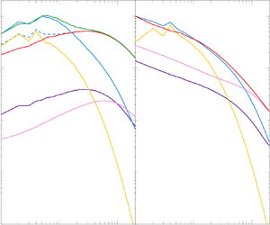
We finally report a simulation (case D) at  $E=E_\eta =10^{-5},$ and a forcing of 10 times critical; figure 4 shows force balances for this simulation. Figure 4(a) is, in many respects, similar to some of the force balances published in the literature for state-of-the-art simulations. A clear crossing is present between the buoyancy and the Lorentz force curves. However, it does not correspond to a dynamically relevant length scale, as revealed by the curl of forces in figure 4(b). In this simulation the solenoidal parts of the buoyancy, Lorentz and Coriolis forces appear to be in general balance, though with some fluctuations. Further work is clearly needed to ascertain whether a more accurate balance of Coriolis and Lorentz forces at all scales (as seen in figure 3e) can be achieved by slightly decreasing
  $E_\eta$ at this value of
  $E$ with fixed forcing.

Figure 4. Force spectra representations for case D.
4. Discussion
We have presented three different representations of force balances in several spherical dynamo simulations. Our length-dependent plots of traditional forces ( $F_l$) are similar to those found previously (Aubert et al. Reference Aubert, Gastine and Fournier2017; Schwaiger et al. Reference Schwaiger, Gastine and Aubert2019; Aubert & Gillet Reference Aubert and Gillet2021; Schwaiger et al. Reference Schwaiger, Gastine and Aubert2021). Broadly speaking,
  $F_l$ is dominated by a zeroth-order geostrophic balance at least at large scales. It can also be argued that, at large scales, a first-order AC
 $^{ag}$ balance then exists. In case B (C) the Lorentz (inertial) force also becomes significant at zeroth order. For case B, the claim could be that a zeroth-order geostrophic balance at large scales gives way to a zeroth-order magnetostrophic balance at smaller scales; however, it is unclear what useful meaning
  $\boldsymbol {F}_{{C}}^{{ag}}$ retains once geostrophy is broken. The remaining forces, namely inertia (in the HD regime and cases A, B and D), Lorentz (in cases A and C) and viscous (in all regimes), appear to be secondary forces across all scales. In particular, the viscous force is always a secondary force in each regime under this representation of the forces. However, this is numerically puzzling as the resolution using a spectral method requires small-scale regularity. The viscous force is thus needed from a numerical point of view to regularise the smallest scales.
Removing the gradient part of each force (including, consequently, the whole pressure gradient force and zeroth-order balance) to form ‘solenoidal forces’ ( $\hat {C}_l$ and
  $P_l$) is desirable because it allows direct access to the balance of forces that controls the dynamics. A projected force
  $P_l$ has a degree of arbitrariness in the choice of the harmonic field, whereas
  $\hat {C}_l$ is uniquely defined. The first-order balance in
  $\hat {C}_l$ and
  $P_l$ is AC at large scales with the Lorentz (inertial) force also entering in case B (C). At smaller scales (near the tail of the spectra), the viscous force now enters the balance in each simulation. When the zeroth-order balance is geostrophic, the leading-order balance in
  $\hat {C}_l$ and
  $P_l$ essentially recovers the first-order balance shown in
  $F_l$. This is because, in such situations, the solenoidal part of the Coriolis force is well approximated by its ageostrophic part; in other words
  $\mathbb {P}(\boldsymbol {F}_{{C}})\approx \boldsymbol {F}_{{C}}^{{ag}}$. However, as
  $l$ increases and
  $\boldsymbol {F}_{{C}}$ loses its predominance in the zeroth-order balance, its ageostrophic part becomes an unreliable approximation for its solenoidal part. We found that
  $\mathbb {P}(\boldsymbol {F}_{{C}})\approx \boldsymbol {F}_{{C}}^{{ag}}$ was only reliably satisfied for
  $l\lesssim 10$; it is a particularly poor measure in case B where the Lorentz force enters the first-order balance even at the largest scales. Notably, this regime is the most relevant for the geodynamo; for this reason we advocate the use of solenoidal forces, which provide an accurate measure for the dynamically relevant balance across all scales. Schwaiger et al. (Reference Schwaiger, Gastine and Aubert2019) and Aubert & Gillet (Reference Aubert and Gillet2021) argue that important length scales for the flow can be derived from the crossings of
  $F_l$ curves. We argue that such crossings of terms containing gradient parts can be misleading when trying to understand the dynamics of an incompressible (Boussinesq) flow. If such crossings are relevant, they should be observed on the curl of forces instead. It is also worth nothing that, in addition to the scale dependence we have presented, force balances may also depend on position; for example, between the regions inside and outside the tangent cylinder. A spectral decomposition, by its nature, cannot capture such inhomogeneity in position.
We constructed two representations of solenoidal forces. Some authors also compare the azimuthal average of the azimuthal component of force balances in order to be free of any gradient effects (this is the case for example in Sheyko et al. (Reference Sheyko, Finlay, Favre and Jackson2018) and Menu, Petitdemange & Galtier (Reference Menu, Petitdemange and Galtier2020)) The advantage of curls is that there is no arbitrariness in the calculation; gradient parts are eliminated in a unique manner. The potential disadvantage of taking curls is their tendency to inflate sharp spatial changes. It is possible to partly compensate  $C_l$ to form
  $\hat {C}_l$; however, this does not account for radial derivatives introduced when curling. Projecting the forces onto their solenoidal part has the advantage of no extra derivative. However, a harmonic field is introduced adding a degree of arbitrariness to
  $P_l$. In our work, the chosen condition on this field was that each force has vanishing radial part on the boundaries. Nevertheless, although plots of
  $\hat {C}_l$ and
  $P_l$ may appear quantitatively different at large scales, they present the same qualitative picture and are equivalent at small scales. In particular, either representation offers a clearer picture of the balance controlling the flow than the comparison of full forces.
Supplementary material
Supplementary material is available at https://doi.org/10.1017/jfm.2023.332.
Acknowledgements
The authors are grateful to S. Tobias for discussions.
Funding
This work was supported by DiRAC Project ACTP245. This work was presented at the Isaac Newton Institute in Cambridge, UK, on 16 May 2022 (E.D.) and on 14 September 2022 (R.J.T.).
Declaration of interests
The authors report no conflict of interest.


 Open access