


1. Introduction
Stability of parallel shear flows of dilute polymer solutions is an outstanding problem of mechanics of complex fluids. While linear stability analyses performed with model viscoelastic fluids suggest that these flows are linearly stable (Gorodtsov & Leonov Reference Gorodtsov and Leonov1967; Wilson, Renardy & Renardy Reference Wilson, Renardy and Renardy1999), it has been proposed that they can lose their stability through a finite-amplitude, sub-critical bifurcation (Morozov & van Saarloos Reference Morozov and van Saarloos2005, Reference Morozov and van Saarloos2007, Reference Morozov and van Saarloos2019), similarly to their Newtonian counterparts (Grossmann Reference Grossmann2000). Recent experiments performed in pressure-driven straight channels support this scenario: for sufficiently high flow rates, there exists a critical strength of flow perturbations required to destabilise the flow (Pan et al. Reference Pan, Morozov, Wagner and Arratia2013), thus demonstrating the sub-critical nature of the transition. Beyond the transition, the flow exhibits features of purely elastic turbulence (Bonn et al. Reference Bonn, Ingremeau, Amarouchene and Kellay2011; Pan et al. Reference Pan, Morozov, Wagner and Arratia2013; Qin & Arratia Reference Qin and Arratia2017), previously reported only in geometries with curved streamlines (Groisman & Steinberg Reference Groisman and Steinberg2000; Steinberg Reference Steinberg2021).
Despite recent progress, the exact origin of purely elastic turbulence remains unknown. One of the major obstacles in understanding its mechanism is the absence of direct numerical simulations of confined flows at sufficiently high flow rates, due to the high Weissenberg number problem (Owens & Phillips Reference Owens and Phillips2002), which is of purely numerical origin. Although significant progress has been made in developing numerical methods capable of controlling this problem (Alves, Oliveira & Pinho Reference Alves, Oliveira and Pinho2021), direct numerical simulations relevant to experiments in parallel shear flows (Bonn et al. Reference Bonn, Ingremeau, Amarouchene and Kellay2011; Pan et al. Reference Pan, Morozov, Wagner and Arratia2013; Qin & Arratia Reference Qin and Arratia2017) are still lacking. Here, we propose to circumvent the high Weissenberg number problem by studying parallel shear flows with free-slip boundary conditions that remove steep near-wall velocity gradients and significantly improve numerical stability.
The influence of wall slip on hydrodynamic stability of various flows has been extensively studied. The motivations behind these studies can be separated into two broad classes. The studies from the first class seek to approximate microscopically sound boundary conditions and thus address the question of linear stability of experimentally realisable flows. Such an approach has indicated, for instance, that the classical two-dimensional Tollmien–Schlichting transition in plane channel flow of Newtonian fluids is significantly suppressed by the presence of wall slip (Gersting Reference Gersting1974; Lauga & Cossu Reference Lauga and Cossu2005; Min & Kim Reference Min and Kim2005), although the non-normal energy growth mechanism was shown to be less affected (Lauga & Cossu Reference Lauga and Cossu2005). When adapted to shear flows of polymeric fluids, this approach revealed the existence of a short-wavelength instability (Black & Graham Reference Black and Graham1996, Reference Black and Graham1999, Reference Black and Graham2001), which is absent in the corresponding no-slip flows.
The second class of studies employs slip boundary conditions exclusively as the means to simplify the underlying no-slip boundary condition problem. The free-slip boundary conditions usually adopted in these works are rather artificial, yet they yield significantly more tractable mathematical problems. This approach was pioneered by Rayleigh (Reference Rayleigh1916) in the context of Rayleigh–Bénard instability. More recently, Waleffe (Reference Waleffe1997) used free-slip boundary conditions to construct exact coherent states in parallel shear flows of Newtonian fluids that revolutionised our understanding of the transition to turbulence in those flows (Eckhardt et al. Reference Eckhardt, Schneider, Hof and Westerweel2007; Tuckerman, Chantry & Barkley Reference Tuckerman, Chantry and Barkley2020; Graham & Floryan Reference Graham and Floryan2021). The most important outcome of these studies is the observation that free-slip systems preserve the main phenomenology of their no-slip counterparts, albeit at increased values of the control parameter. Our work draws its motivation from this class of studies.
Here, we perform a linear stability analysis of plane Couette flow (pCF) and pressure-driven plane Poiseuille flow (pPF) with free-slip boundary conditions. We employ the Oldroyd-B model (Bird, Armstrong & Hassager Reference Bird, Armstrong and Hassager1987) in the absence of inertia, and demonstrate numerically that these flows develop linear instabilities absent in their no-slip counterparts. Importantly, we observe that the main features of no-slip flows are preserved under the free-slip conditions, and we discuss how these instabilities can be employed to gain insight into the nature of elastic turbulence in parallel geometries.
2. Problem set-up
We study incompressible flows of a model viscoelastic fluid confined between two infinite parallel plates. We introduce a Cartesian coordinate system  $\{x_1,x_2,x_3\}$ oriented along the streamwise, gradient and spanwise directions, respectively; the plates are located at
  $x_2=\pm L$. The dynamics of the fluid is assumed to be described by the Oldroyd-B model (Bird et al. Reference Bird, Armstrong and Hassager1987),
 $$\begin{gather} {\boldsymbol \tau} + Wi \left[ \frac{\partial {\boldsymbol \tau}}{\partial t} + {\boldsymbol v}\boldsymbol{\cdot}\boldsymbol{\nabla}{\boldsymbol \tau} - \left(\boldsymbol{\nabla} {\boldsymbol v}\right)^{\rm T}\boldsymbol{\cdot}{\boldsymbol \tau} - {\boldsymbol \tau}\boldsymbol{\cdot}\left(\boldsymbol{\nabla} {\boldsymbol v}\right)\right] = \left(\boldsymbol{\nabla} {\boldsymbol v}\right) + \left(\boldsymbol{\nabla} {\boldsymbol v}\right)^{\rm T}, \end{gather}$$
 $$\begin{gather}Re \left[ \frac{\partial {\boldsymbol v}}{\partial t} + {\boldsymbol v}\boldsymbol{\cdot}\boldsymbol{\nabla}{\boldsymbol v} \right] ={-}\boldsymbol{\nabla} p + \beta \boldsymbol{\nabla}^2{\boldsymbol v} + (1-\beta)\boldsymbol{\nabla}\boldsymbol{\cdot}{\boldsymbol \tau} + {\boldsymbol f}, \end{gather}$$
 $$\begin{gather}\boldsymbol{\nabla}\boldsymbol{\cdot} {\boldsymbol v} = 0, \end{gather}$$
where  $\boldsymbol v$,
  $\boldsymbol \tau$ and
  $p$ are the fluid velocity, the polymeric Cauchy stress tensor and the pressure, respectively, while
  $(\boldsymbol {\nabla } {\boldsymbol v})^{\rm T}$ denotes the transpose of the velocity gradient tensor;
  $\boldsymbol f$ is a body force to be specified below. These equations are rendered dimensionless using the channel's half-width
  $L$ as the unit of length, the maximum velocity of the laminar profile
  $V_0$ as the unit velocity, and
  $L/V_0$ as the unit of time. The governing equations (2.1) feature three dimensionless groups, the Weissenberg number
  $Wi=\lambda V_0/L$, the Reynolds number
  $Re= \rho L V_0/\eta$ and the viscosity ratio
  $\beta =\eta _s/\eta$, where
  $\lambda$ is the Maxwell relaxation time of the fluid,
  $\rho$ is its density, and
  $\eta _s$ and
  $\eta$ are the solvent viscosity and the total viscosity of the fluid, respectively. Unless stated otherwise, below we focus on the purely elastic limit with
  $Re=0$.
The fluid is assumed to satisfy the following free-slip boundary conditions at the walls:
 \begin{equation} \partial_2 v_1 = v_2 = \partial_2 v_3 = 0, \quad \text{for }x_2={\pm} 1,\end{equation}
where  $\partial _2$ denotes the spatial derivative in the gradient direction. In this work, we study unidirectional laminar profiles
  ${\boldsymbol v} = \{U(x_2),0,0\}$, where
  $U$ is chosen to resemble the shape and symmetry of either plane Poiseuille flow (pPF) or plane Couette flow (pCF), while satisfying the boundary conditions (2.2):
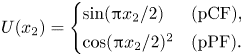 \begin{equation} U(x_2) = \begin{cases}
\sin({\rm \pi} x_2/2) & \text{(pCF),} \\[2pt] \cos({\rm \pi}
x_2/2)^2 & \text{(pPF).}
\end{cases}\end{equation}
\begin{equation} U(x_2) = \begin{cases}
\sin({\rm \pi} x_2/2) & \text{(pCF),} \\[2pt] \cos({\rm \pi}
x_2/2)^2 & \text{(pPF).}
\end{cases}\end{equation}
The corresponding laminar components of the polymeric stress tensor are given by  $\tau _{11} = 2 Wi(\partial _2 U(x_2))^2$ and
  $\tau _{12} = \partial _2 U(x_2)$, with all other components being zero. To drive such flows in the presence of free-slip boundary conditions, we add the body force
  ${\boldsymbol f} = \{-\partial _2^2 U(x_2),0,0\}$ to the right-hand side of (2.1b).
To perform a linear stability analysis of these flows, we linearise the equations (2.1) around the laminar profile given above. In view of the viscoelastic analogue of Squire's theorem (Bistagnino et al. Reference Bistagnino, Boffetta, Celani, Mazzino, Puliafito and Vergassola2007), which also holds for the free-slip boundary conditions studied here, we consider two-dimensional modal perturbations  $\{\delta {\boldsymbol v}(x_2), \delta {\boldsymbol \tau }(x_2), \delta p(x_2) \} \, \textrm {e}^{\textrm {i} k_1 x_1} \, \textrm {e}^{\sigma t}$ of the velocity, stress and pressure, respectively. Here,
  $k_1$ sets the spatial scale of the perturbation, and
  $\sigma =\sigma _r + i \sigma _i$ denotes a complex temporal eigenvalue, with
  $\sigma _r$ and
  $\sigma _i$ being its real and imaginary part, respectively. The
  $x_2$ dependences of the perturbations are expanded in Chebyshev polynomials, and the linearised equations of motion are solved with a fully spectral Chebyshev–Tau method (Canuto et al. Reference Canuto, Hussaini, Quarteroni and Zang1987) by employing the generalised eigenvalue solver eig from the scientific library SciPy for Python (Virtanen et al. Reference Virtanen2020).
3. Results
The no-slip pCF and pPF of Oldroyd-B fluids are linearly stable for a wide range of  $\beta$ and
  $Wi$ (Gorodtsov & Leonov Reference Gorodtsov and Leonov1967; Wilson et al. Reference Wilson, Renardy and Renardy1999). Recently Khalid, Shankar & Subramanian (Reference Khalid, Shankar and Subramanian2021b) reported a purely elastic linear instability in no-slip pPF; however, its region of existence is confined to a small and, most likely, experimentally inaccessible part of the parameter space with
  $\beta >0.9$ and
  $Wi>O(10^3)$. Surprisingly, here we find that free-slip pCF and pPF are linearly unstable for a wide range of
  $\beta$ and
  $Wi$.
$Wi$.
In figure 1, we present examples of such instabilities by plotting the eigenvalue spectra for pCF and pPF. Similarly to those of the no-slip problem (Wilson et al. Reference Wilson, Renardy and Renardy1999), the spectra consist of discrete physical eigenvalues and two lines of eigenvalues corresponding to continuous spectra with  $\sigma _r=-1/Wi$ and
  $\sigma _r = -1/(\beta Wi)$; the finite-resolution approximations to the latter take the balloon-like shapes visible in figure 1. The most profound feature of both spectra in figure 1 is that all leading eigenvalues have positive real parts, indicating the presence of a linear instability. Surprisingly, two of the three leading eigenvalues in pPF have numerically almost identical real parts for all values of the parameters we considered (see also figure 6 below).
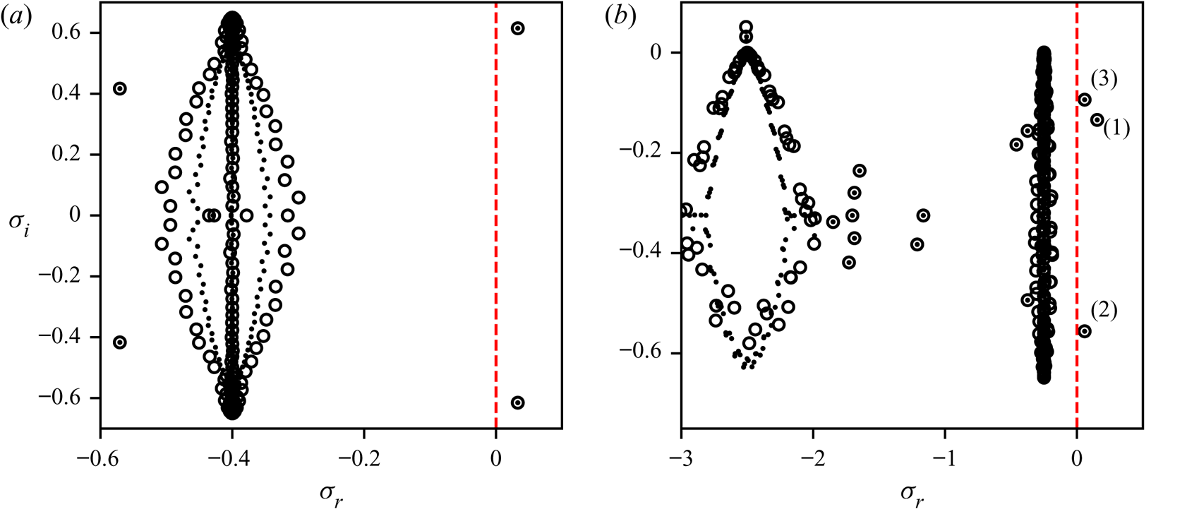
Figure 1. Eigenvalue spectra for  $\beta =0.1$ and
  $k_1=0.65$ for (a) pCF at
  $Wi=2.5$, and (b) pPF at
  $Wi=4.0$. The dashed red lines denote marginal stability. Both figures compare spectra calculated with
  $50$ (open circles) and
  $100$ (dots) Chebyshev polynomials.
To demonstrate numerical convergence, in figure 1 we present the eigenvalue spectra for two spectral resolutions, with  $M=50$ and
  $M=100$ Chebyshev polynomials, respectively, and observe that the physical eigenvalues are well-converged. All calculations presented below are therefore carried out with
  $M=50$. While this spectral resolution is quite low to yield converged results in the no-slip setting (Wilson et al. Reference Wilson, Renardy and Renardy1999; Khalid et al. Reference Khalid, Shankar and Subramanian2021b), it is clearly sufficient for the free-slip boundary conditions. This observation supports our original rationale that the free-slip boundary conditions simplify numerical simulations of such flows by removing steep near-wall velocity gradients.
For no-slip boundary conditions, the least stable eigenmode of pCF and one of the three leading eigenmodes of pPF are mostly localised in the vicinity of the confining boundaries (Gorodtsov & Leonov Reference Gorodtsov and Leonov1967; Wilson et al. Reference Wilson, Renardy and Renardy1999), and are thus referred to as wall modes, while the other two pPF modes are mostly localised in the bulk (Wilson et al. Reference Wilson, Renardy and Renardy1999; Khalid et al. Reference Khalid, Shankar and Subramanian2021b), i.e. they are centre modes. In figure 2 we present the spatial profiles corresponding to the unstable free-slip eigenvalues discussed above, and observe that the distinction between wall and centre mode is significantly weakened. Although the symmetries of the stress distribution and the streamfunction are still different between these modes (compare the vortex structure in figure 2(a,b) with (c,d), for instance), all modes now have significant presence throughout the domain. Notably, the fact that all these modes can be simultaneously unstable indicates the presence of several, rather different instability mechanisms.
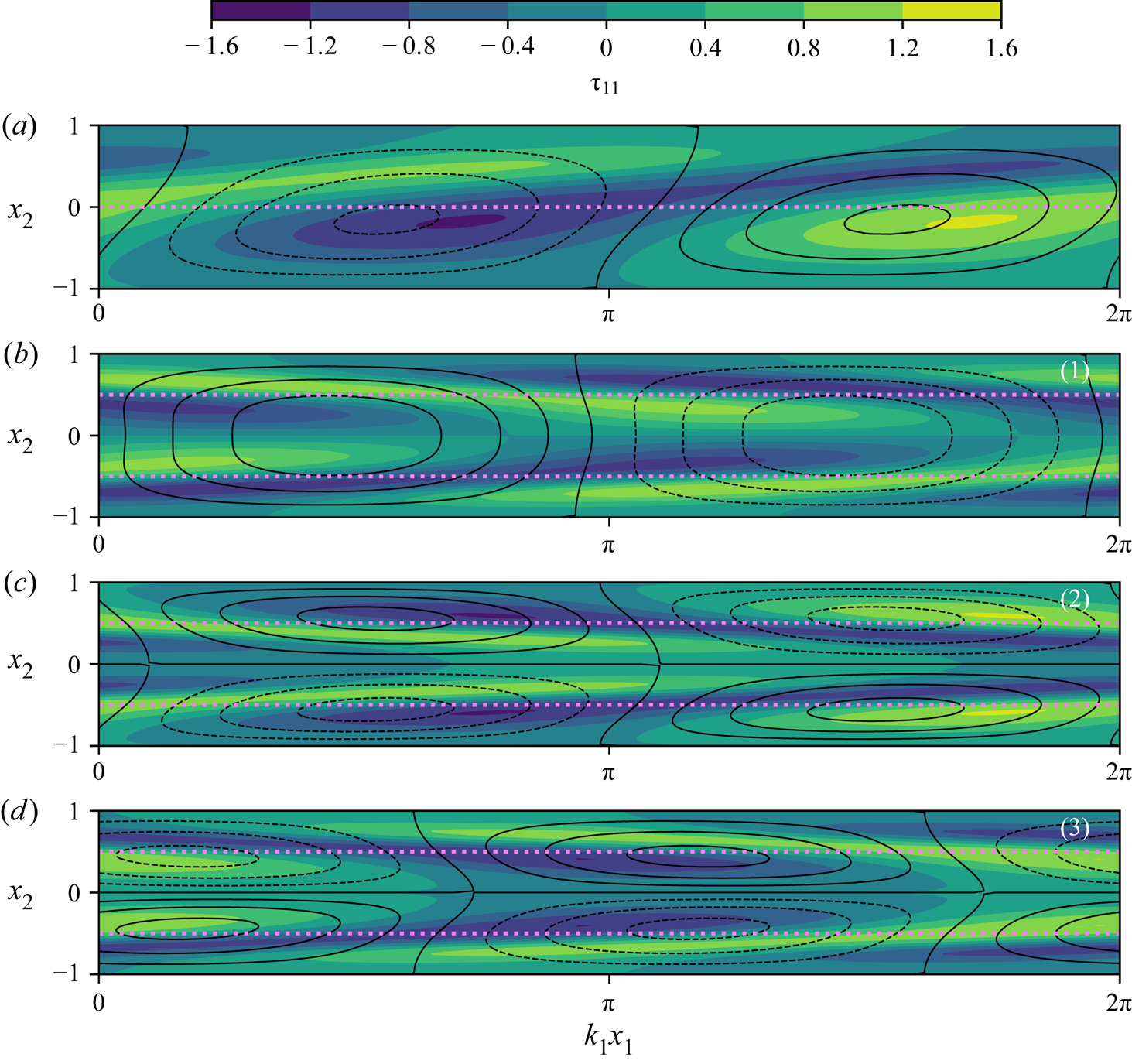
Figure 2. Spatial profiles of the polymeric stress  $\delta \tau _{11}$ (colour) and the streamfunction (contours with negative values denoted by dashed lines) corresponding to the unstable eigenvalues in figure 1 for
  $\beta =0.1$ and
  $k_1=0.65$: (a) pCF at
  $Wi=2.5$; (b)–(d) pPF eigenmodes (1)–(3) at
  $Wi=4.0$ (see figure 1b). The violet dotted lines denote the positions of the maxima of the base components
  $\vert \tau _{12}\vert$ and
  $\vert \tau _{11}\vert$.
In figure 3 we present the neutral stability curves for various values of  $\beta$, while figure 4 shows the critical Weissenberg number
  $Wi_{c}$ and the corresponding critical wavenumber
  $k_{1,c}$ as functions of
  $\beta$. The neutral stability curves are skewed towards small values of
  $k_1$ in a way reminiscent of the elasto-inertial (Chaudhary et al. Reference Chaudhary, Garg, Shankar and Subramanian2019; Khalid et al. Reference Khalid, Chaudhary, Garg, Shankar and Subramanian2021a) and purely elastic modes (Khalid et al. Reference Khalid, Shankar and Subramanian2021b) discovered recently. Despite these similarities, we were unable to use the re-scaling procedure proposed in those works to collapse all our neutral stability data on a single master curve. Furthermore, in figure 4(a) we observe that
  $Wi_c$ increases rapidly as
  $\beta \to 1$, indicating that a sufficiently strong velocity–stress coupling is required to drive the instability. We also note that
  $Wi_c$ is significantly smaller for pPF than for pCF, and that, surprisingly, the critical wavenumber
  $k_{1,c}$ depends in different ways on
  $\beta$ for these flows. As can be seen in figure 4(b), in all cases,
  $k_{1,c}\sim O(1)$, indicating an instability length scale comparable with the wall-to-wall distance.
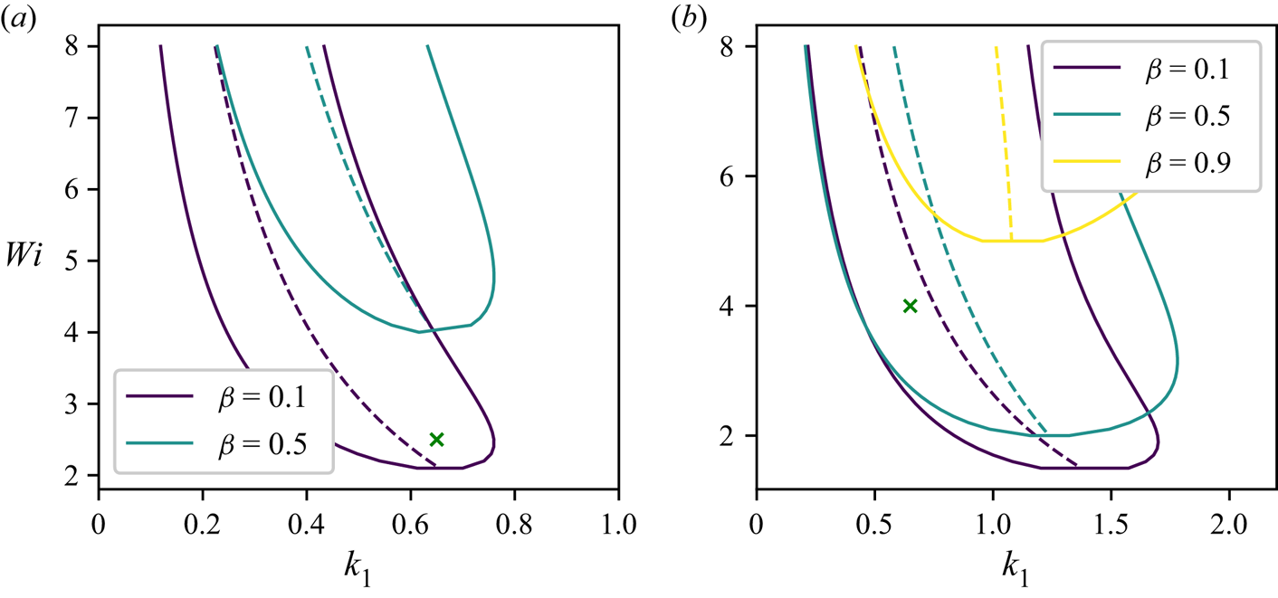
Figure 3. Neutral stability curves (solid lines) and the positions of the most unstable eigenvalue maxima (dashed lines) for (a) pCF and (b) pPF. The green crosses correspond to the parameters used in figure 1.
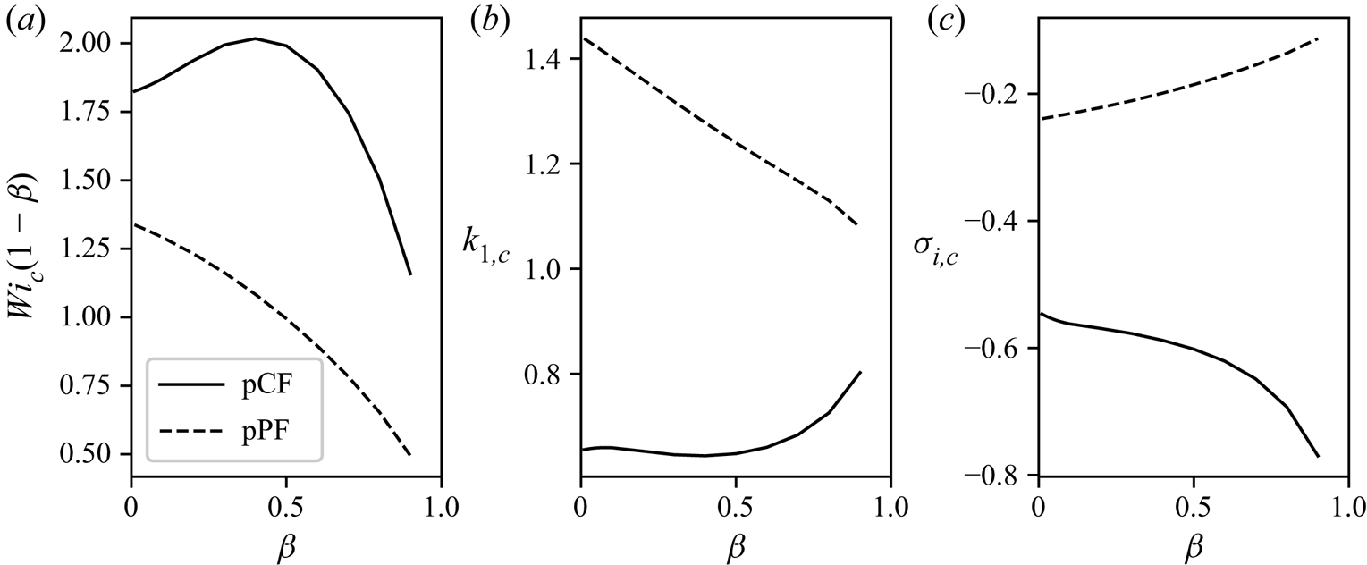
Figure 4. (a) The critical Weissenberg number  $Wi_c$ as a function of
  $\beta$. (b) The corresponding critical wavenumber
  $k_{1,c}$, and (c) the imaginary part of the critical eigenvalue
  $\sigma _{i,c}$, as a function of
  $\beta$.
To assess the influence of weak inertia, in figure 5 we plot the leading eigenvalue of pCF and pPF as a function of the Reynolds number. We see that while small amounts of inertia have a stabilising effect on pCF, the low- $\beta$ instabilities in pPF are only mildly suppressed. For pPF at sufficiently high
  $\beta$, the trend reverses, and we observe a stable purely elastic eigenmode becoming unstable for
  $Re>0$. While a full
  $Wi-\beta -Re$ critical surface is required to draw a definite conclusion regarding the influence of inertia on each mode, we note here that our observations are in line with the recent work on elasto-inertial instabilities (Chaudhary et al. Reference Chaudhary, Garg, Shankar and Subramanian2019; Khalid et al. Reference Khalid, Chaudhary, Garg, Shankar and Subramanian2021a).
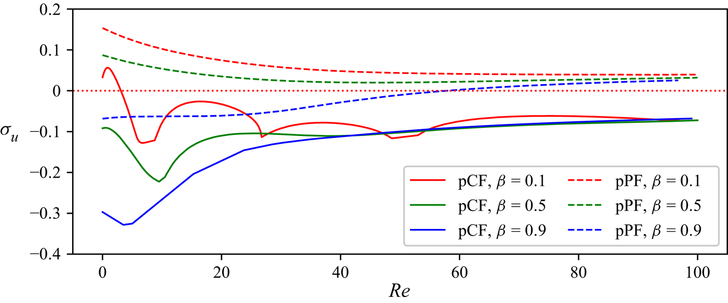
Figure 5. Influence of weak inertia on linear instability of pCF and pPF at  $Wi=2.5$ and
  $Wi=4.0$, respectively, at
  $k_1=0.65$ as denoted by the green cross in figure 3. The dotted red line denotes marginal stability.
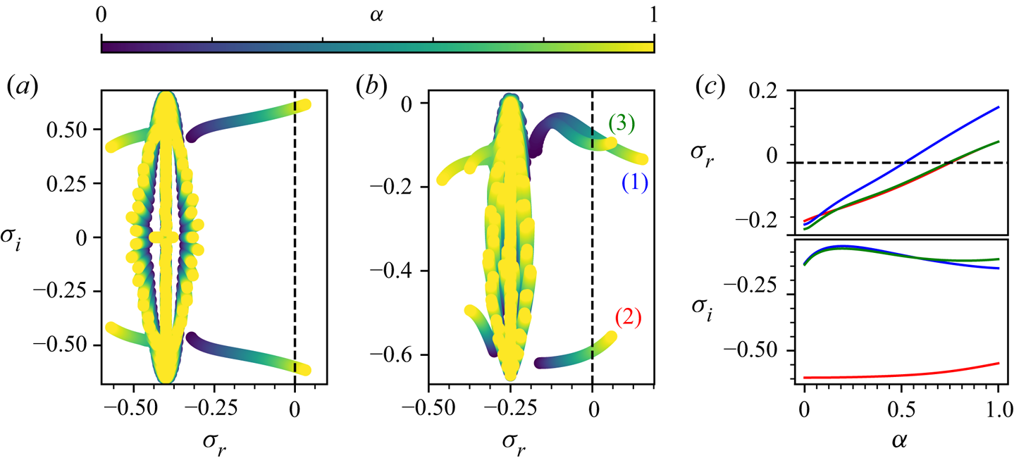
Figure 6. (a,b) Eigenvalue spectrum of system with continuously varied boundary conditions from free-slip (yellow) to no-slip (violet) for (a) pCF at  $Wi=2.5$ and (b) pPF at
  $Wi=4.0$. Data shown in both panels were calculated for
  $\beta =0.1$,
  $Re=0.0$ and
  $k_1=0.65$. The black dashed line denotes marginal stability. Each spectrum is colour-coded according to the value of the homotopy parameter
  $\alpha$. (c) Real and imaginary parts of the three leading eigenvalues from (b) as a function of
  $\alpha$. The dashed line denotes the instability threshold. The leading pCF eigenvalues (not shown) become stable for
  $\alpha <0.88$, while the leading pPF eigenvalues (1), (2) and (3) become stable for
  $\alpha <0.52$,
  $0.75$ and
  $0.74$, respectively.
The spectra presented in figure 1 bear a striking resemblance to the spectra of the corresponding flows of Oldroyd-B fluids with no-slip boundary conditions (Gorodtsov & Leonov Reference Gorodtsov and Leonov1967; Wilson et al. Reference Wilson, Renardy and Renardy1999) but for the position of the leading eigenvalues, which appear to move to positive values of  $\sigma _r$ in the free-slip case. To establish a connection between these eigenvalues and their no-slip counterparts, we perform a homotopy between the two types of boundary conditions. To this end, we introduce a laminar profile that depends on a parameter
  $\alpha$,
 \begin{equation} U(x_2) = \begin{cases}
\alpha \sin({\rm \pi} x_2/2) + (1-\alpha) x_2 &
\text{(pCF),} \\[3pt] \alpha \cos({\rm \pi} x_2/2)^2 + (1-\alpha)
(1-x_2^2) & \text{(pPF),}
\end{cases}\end{equation}
\begin{equation} U(x_2) = \begin{cases}
\alpha \sin({\rm \pi} x_2/2) + (1-\alpha) x_2 &
\text{(pCF),} \\[3pt] \alpha \cos({\rm \pi} x_2/2)^2 + (1-\alpha)
(1-x_2^2) & \text{(pPF),}
\end{cases}\end{equation}
which interpolates between (2.3) ( $\alpha =1$) and the classical no-slip pCF and pPF profiles (
 $\alpha =0$). A similar interpolation is imposed on the boundary conditions:
 \begin{equation} \alpha \partial_2 \delta v_1 \pm (1-\alpha) \delta v_1 = v_2 = \alpha \partial_2 \delta v_3 \pm (1-\alpha) \delta v_3 = 0, \quad \text{for }x_2={\pm} 1. \end{equation}
In figure 6 we show the superimposed spectra for this laminar profile as a function of  $\alpha$ for pCF and pPF. The results of the homotopy procedure clearly indicate that the unstable modes do not appear either from infinity or from the continuous spectra, but instead are continuously connected to the well-known least stable eigenvalues of no-slip parallel shear flows (Gorodtsov & Leonov Reference Gorodtsov and Leonov1967; Wilson et al. Reference Wilson, Renardy and Renardy1999).
4. Conclusions
In this work, we demonstrate that free-slip pCF and pPF of Oldroyd-B fluids are linearly unstable. The instabilities we observe are caused neither by the curvature of the base flow streamlines, where hoop stresses are known to lead to purely elastic instabilities (McKinley, Pakdel & Öztekin Reference McKinley, Pakdel and Öztekin1996), nor by steep gradients of the material properties, as in the co-extrusion problems (Hinch, Harris & Rallison Reference Hinch, Harris and Rallison1992). Suggestively, the base velocity profiles considered here change the sign of their second derivatives inside the domain, which might indicate a connection to Rayleigh's inflection point instability criterion for inviscid fluids (Drazin & Reid Reference Drazin and Reid2004). A similar situation occurs in purely elastic Kolmogorov flows (Boffetta et al. Reference Boffetta, Celani, Mazzino, Puliafito and Vergassola2005), and it would be interesting to examine whether the instabilities observed there are related to those found in this work. By performing a homotopy between free-slip and no-slip boundary conditions, we demonstrate that the unstable eigenmodes are directly related to the least stable modes of the no-slip system. The exact way by which the introduction of an inflection point into the base profile would lead to destabilisation of the no-slip modes is currently unknown.
While the body forcing and the boundary conditions considered here are probably difficult, if not impossible, to realise in practice, the main importance of our work is not related to its direct experimental relevance. Instead, our contribution here is related to the observation that the free-slip problem considered here is significantly simpler to address numerically than its no-slip counterpart. Even at the linear level, a significantly lower number of Chebyshev modes is needed to resolve the eigenspectrum than in the no-slip case. A similar simplification is also expected to occur in fully nonlinear direct numerical simulations and to alleviate the high Weissenberg number problem plaguing such studies. By rendering the leading eigenmodes unstable, free-slip flows offer an easier route to the study of strongly sub-critical structures that propagate from those eigenmodes in the no-slip case (Morozov & van Saarloos Reference Morozov and van Saarloos2005, Reference Morozov and van Saarloos2007, Reference Morozov and van Saarloos2019).
Once coherent states are resolved in direct numerical simulations of free-slip flows, a boundary condition homotopy similar to the one employed here can be used to track those solutions back to the no-slip conditions (Waleffe Reference Waleffe2003). Recent work on elasto-inertial parallel shear flows (Garg et al. Reference Garg, Chaudhary, Khalid, Shankar and Subramanian2018; Chaudhary et al. Reference Chaudhary, Garg, Shankar and Subramanian2019, Reference Chaudhary, Garg, Subramanian and Shankar2021; Khalid et al. Reference Khalid, Chaudhary, Garg, Shankar and Subramanian2021a) associates linear instabilities at high  $Wi$ and
  $Re$ with the very leading eigenvalues studied here. As already mentioned above, the same instability can be traced to the purely elastic case,
  $Re=0$, for sufficiently large values of
  $\beta$ and
  $Wi$ (Khalid et al. Reference Khalid, Shankar and Subramanian2021b). It has also been shown that these instabilities are sub-critical in nature (Page, Dubief & Kerswell Reference Page, Dubief and Kerswell2020). Taken together with the original proposal of Morozov & van Saarloos (Reference Morozov and van Saarloos2005, Reference Morozov and van Saarloos2007, Reference Morozov and van Saarloos2019) and the experimental and numerical studies of nonlinear states in elasto-inertial flows (Dubief, Terrapon & Soria Reference Dubief, Terrapon and Soria2013; Samanta et al. Reference Samanta, Dubief, Holzner, Schäfer, Morozov, Wagner and Hof2013; Choueiri, Lopez & Hof Reference Choueiri, Lopez and Hof2018; Sid, Terrapon & Dubief Reference Sid, Terrapon and Dubief2018; Lopez, Choueiri & Hof Reference Lopez, Choueiri and Hof2019), this points towards the existence of exact coherent states related to the least stable eigenvalues, even though they are linearly stable for most values of
  $\beta$ and
  $Wi$. Our work suggests using a homotopy from free-slip flows to discover these structures.
Finally, we note that our results suggest that all three leading eigenvalues of free-slip pPF can become unstable; see figure 1, for example. In elasto-inertial flows, there is an ongoing discussion whether the most dynamically relevant coherent structures are related to wall or centre-line modes (Shekar et al. Reference Shekar, McMullen, Wang, McKeon and Graham2019; Datta et al. Reference Datta2021). In figure 7, we present the neutral stability curve for the first three eigenvalues and observe that by selecting the wavenumber and the Weissenberg number, one can control the type of the instability thus produced. As figure 2 suggests, the different spatial symmetries of those modes should result in structures that connect to either wall or centre-line modes, when traced back to the no-slip conditions, thus allowing one to assess their relative importance independently.
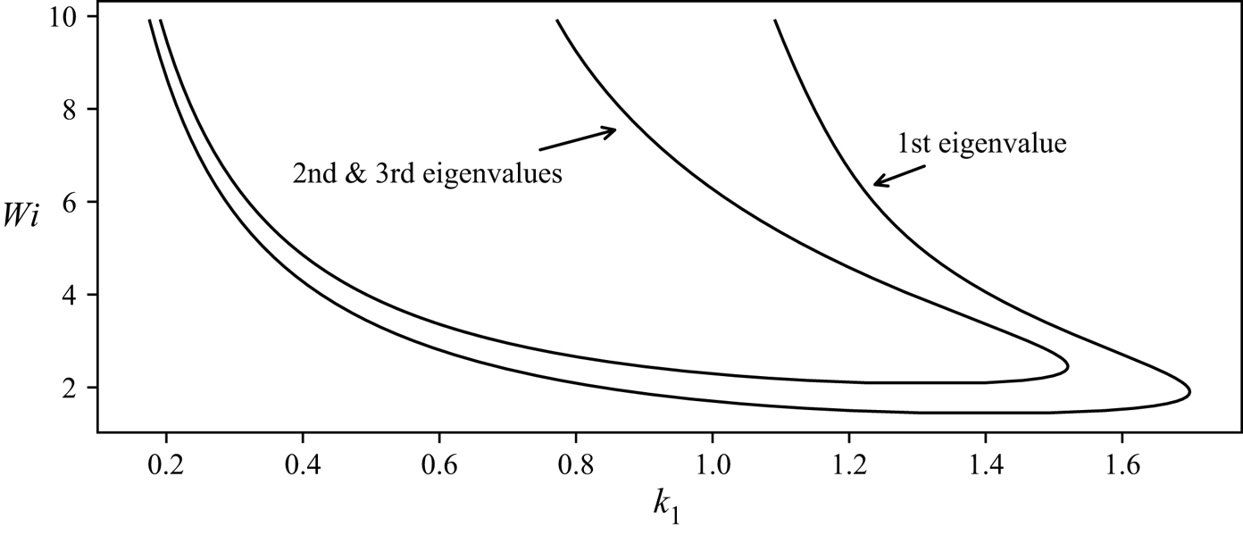
Figure 7. Neutral stability curves of the first three eigenvalues of pPF for  $\beta =0.1$. As mentioned in § 3, the second and third eigenvalues have the same real parts, and their instability regions coincide.
Acknowledgements
Professor Eckhardt took active part in conceiving this project and interpreting the free-slip plane Couette flow results. He did not see the part of this work on plane Poiseuille flow, which we hope we continued in line with his high scientific standards. All shortcomings should be attributed to A.M.
Declaration of interest
The authors report no conflict of interest.


 Open access