


1. Introduction
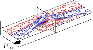
We consider a specific case of heterogeneous roughness where the roughness varies in the spanwise direction. Spanwise heterogeneity is imposed by alternating rough and smooth strips to form a test surface over which a turbulent boundary layer is developed (figure 2). This type of roughness heterogeneity induces secondary flows in the form of counter-rotating streamwise rollers, which are apparent in the time-averaged velocity field. An examination of the instantaneous velocity field, however, reveals the secondary flows as elongated meandering high- and low-speed streaks, not unlike the large-scale/very-large-scale motions (LSMs/VLSMs) that occur naturally in wall-bounded turbulence. Throughout this study, we refer to ‘secondary flows’ as structures generated by spanwise heterogeneity, and ‘large-scale structures’ or LSMs as those which naturally occur in wall-bounded turbulence.
LSMs have commonly been associated with hairpin packets (Adrian, Meinhart & Tomkins Reference Adrian, Meinhart and Tomkins2000; Tomkins & Adrian Reference Tomkins and Adrian2003) and  $\delta$-scaled meandering high- and low-momentum streaks (Hutchins & Marusic Reference Hutchins and Marusic2007a,Reference Hutchins and Marusicb) in the outer layer of wall-bounded turbulent flows, where
  $\delta$ is either the boundary-layer thickness, channel half-height or pipe radius. In the logarithmic region, clusters of hairpin packets agglomerate to form VLSMs or ‘superstructures’ (Kim & Adrian Reference Kim and Adrian1999; Guala, Hommema & Adrian Reference Guala, Hommema and Adrian2006; Balakumar & Adrian Reference Balakumar and Adrian2007; Hutchins & Marusic Reference Hutchins and Marusic2007a; Dennis & Nickels Reference Dennis and Nickels2011b; Lee & Sung Reference Lee and Sung2011; Hutchins et al. Reference Hutchins, Chauhan, Marusic, Monty and Klewicki2012; Wu, Baltzer & Adrian Reference Wu, Baltzer and Adrian2012). The imprint of symmetrical hairpin vortex packets is evident in certain statistical analyses of these structures. For example, two-point correlations of the fluctuating flow field exhibit an elongated low-momentum streak flanked by high-momentum streaks in the spanwise direction (Ganapathisubramani, Longmire & Marusic Reference Ganapathisubramani, Longmire and Marusic2003; Tomkins & Adrian Reference Tomkins and Adrian2003; Ganapathisubramani et al. Reference Ganapathisubramani, Hutchins, Hambleton, Longmire and Marusic2005; Hutchins, Hambleton & Marusic Reference Hutchins, Hambleton and Marusic2005; Hutchins & Marusic Reference Hutchins and Marusic2007a; Marusic, Mathis & Hutchins Reference Marusic, Mathis and Hutchins2010; Dennis & Nickels Reference Dennis and Nickels2011a). However, Johansson, Alfredsson & Kim (Reference Johansson, Alfredsson and Kim1991) cautioned against this interpretation of the two-point correlation contours. Ensemble averaging and assumptions of spanwise homogeneity, as typically applied in the computation for smooth wall-bounded turbulence, enforce a plane of symmetry in the resulting conditional average. Asymmetrical large-scale structures (one-sided roll modes) have, in fact, been observed instantaneously in turbulent boundary layers formed over smooth walls (Lozano-Durán, Flores & Jiménez Reference Lozano-Durán, Flores and Jiménez2012; Kevin, Monty & Hutchins Reference Kevin, Monty and Hutchins2019a), heterogeneous roughness (Vanderwel et al. Reference Vanderwel, Stroh, Kriegseis, Frohnapfel and Ganapathisubramani2019; Wangsawijaya et al. Reference Wangsawijaya, Baidya, Chung, Marusic and Hutchins2020) and converging–diverging (C–D) riblets (Kevin et al. Reference Kevin, Monty, Bai, Pathikonda, Nugroho, Barros, Christensen and Hutchins2017). Elsinga et al. (Reference Elsinga, Adrian, Van Oudheusden and Scarano2010) observed that hairpin packets are most likely comprised of arch-like or cane-shaped structures. Similar to the near-wall cycle, an alternative model for the formation mechanism has been suggested for coherent structures in the outer layer. Large-scale elongated streaks with a sinuous instability and associated asymmetric staggered quasi-streamwise vortices have been observed in the logarithmic region and beyond (Flores & Jiménez Reference Flores and Jiménez2010; Cossu & Hwang Reference Cossu and Hwang2017; de Giovanetti, Sung & Hwang Reference de Giovanetti, Sung and Hwang2017), which are similar to, but at a much larger scale than, structures associated with the streak-vortex instability, which was initially developed as a model for near-wall streak formation (Jeong et al. Reference Jeong, Hussain, Schoppa and Kim1997; Waleffe Reference Waleffe2001; Schoppa & Hussain Reference Schoppa and Hussain2002).
The secondary flows are regarded as a result of production–dissipation imbalance of turbulent kinetic energy induced by spanwise heterogeneity (Hinze Reference Hinze1967). For a surface comprised of spanwise-alternating rough–smooth strips, production exceeds dissipation above the rough strips, and vice versa for the smooth strips, resulting in counter-rotating secondary flows, with upwelling above the smooth strips and downwelling above the rough strips. Within the flow, these are associated with the formation of low-momentum pathways and high-momentum pathways (for upwelling and downwelling, respectively (Barros & Christensen Reference Barros and Christensen2014; Willingham et al. Reference Willingham, Anderson, Christensen and Barros2014; Anderson et al. Reference Anderson, Barros, Christensen and Awasthi2015). Previous studies have shown that spacing/roughness strip width dictates the behaviour of the (time-averaged) secondary flows. In general, three regimes of the flow, differently affected by the resulting secondary flows, have been observed: where the strip width  $S$ is either larger/much larger than
  $\delta$ (
 $S/\bar {\delta } \gg 1$), comparable to
  $\delta$ (
 $S/\bar {\delta } \approx 1$) and smaller/much smaller than
  $\delta$ (
 $S/\bar {\delta } \ll 1$) (Chung, Monty & Hutchins Reference Chung, Monty and Hutchins2018; Medjnoun, Vanderwel & Ganapathisubramani Reference Medjnoun, Vanderwel and Ganapathisubramani2018; Yang & Anderson Reference Yang and Anderson2018). In the regime where
  $S/\delta \gg 1$, domain-sized secondary flows are observed (Yang & Anderson Reference Yang and Anderson2018), along with the recovery to outer layer similarity at spanwise locations far removed from the secondary flows (Chung et al. Reference Chung, Monty and Hutchins2018). This regime has been referred to as the ‘heterogeneity’ regime by Yang & Anderson (Reference Yang and Anderson2018). In the intermediate regime (
 $S/\delta \approx 1$), the flow becomes truly ‘heterogeneous’ as the secondary flows occupy the entire space provided by the boundary layer/channel (Medjnoun et al. Reference Medjnoun, Vanderwel and Ganapathisubramani2018). This regime has been referred to as ‘transitional’ by Yang & Anderson (Reference Yang and Anderson2018) or the ‘intermediate’ regime by Chung et al. (Reference Chung, Monty and Hutchins2018) and Wangsawijaya et al. (Reference Wangsawijaya, Baidya, Chung, Marusic and Hutchins2020). Here, the strength of the secondary flows is most significant compared with the other two regimes (Vanderwel & Ganapathisubramani Reference Vanderwel and Ganapathisubramani2015; Yang & Anderson Reference Yang and Anderson2018; Medjnoun et al. Reference Medjnoun, Vanderwel and Ganapathisubramani2018; Chung et al. Reference Chung, Monty and Hutchins2018; Wangsawijaya et al. Reference Wangsawijaya, Baidya, Chung, Marusic and Hutchins2020), and so is the skin friction drag (Chung et al. Reference Chung, Monty and Hutchins2018; Medjnoun et al. Reference Medjnoun, Vanderwel and Ganapathisubramani2018). Two phenomena have been documented in the previous studies within this intermediate regime. Firstly, the flow slows down above the smooth instead of rough strips, as opposed to the limiting case behaviour observed for
  $S/\bar {\delta } \gg 1$ (Chung et al. Reference Chung, Monty and Hutchins2018; Xie, Chung & Hutchins Reference Xie, Chung and Hutchins2020; Wangsawijaya et al. Reference Wangsawijaya, Baidya, Chung, Marusic and Hutchins2020). Secondly, for ridges (where secondary flows are induced by spanwise variation in the virtual origin), reversal of the secondary flow direction has also been documented (Yang & Anderson Reference Yang and Anderson2018). As
  $S$ decreases further (
 $S/\delta \ll 1$), the size of the secondary flow diminishes and these flows are constrained close to the surface, with the flow approaching a ‘homogeneous’ roughness state away from the surface (Yang & Anderson Reference Yang and Anderson2018). Here, the region close to the surface containing secondary flows is analogous to the roughness sublayer, beyond which we would expect the flow to approach spanwise homogeneity (Chan et al. Reference Chan, MacDonald, Chung, Hutchins and Ooi2018; Chung et al. Reference Chung, Monty and Hutchins2018).
Instantaneously, the secondary flows and the naturally occurring large-scale structures share some similarities, as both are characterised by roll modes and elongated high- and low-momentum streaks. The LSM/VLSM exhibits a known streamwise coherence between 3 $\delta$ (Kovasznay, Kibens & Blackwelder Reference Kovasznay, Kibens and Blackwelder1970; Guala et al. Reference Guala, Hommema and Adrian2006) up to 20
 $\delta$ (Hutchins & Marusic Reference Hutchins and Marusic2007a). The secondary flow emerging from surface roughness heterogeneity investigated here, on the other hand, has a streamwise infinite mode in the time-averaged sense. However, there is also evidence that these secondary flows have a time-dependent and spatially varying form (Anderson Reference Anderson2019; Vanderwel et al. Reference Vanderwel, Stroh, Kriegseis, Frohnapfel and Ganapathisubramani2019; Wangsawijaya et al. Reference Wangsawijaya, Baidya, Chung, Marusic and Hutchins2020). This behaviour can be inferred from the one-dimensional (1-D) energy spectrograms (Nugroho, Hutchins & Monty Reference Nugroho, Hutchins and Monty2013; Awasthi & Anderson Reference Awasthi and Anderson2018; Medjnoun et al. Reference Medjnoun, Vanderwel and Ganapathisubramani2018; Zampiron, Cameron & Nikora Reference Zampiron, Cameron and Nikora2020; Wangsawijaya et al. Reference Wangsawijaya, Baidya, Chung, Marusic and Hutchins2020), two-point correlation maps (Kevin et al. Reference Kevin, Monty, Bai, Pathikonda, Nugroho, Barros, Christensen and Hutchins2017; Kevin, Monty & Hutchins Reference Kevin, Monty and Hutchins2019b; Wangsawijaya et al. Reference Wangsawijaya, Baidya, Chung, Marusic and Hutchins2020), and POD (proper orthogonal decomposition) of the turbulent fluctuation fields (Vanderwel et al. Reference Vanderwel, Stroh, Kriegseis, Frohnapfel and Ganapathisubramani2019). Time dependence of secondary flows has been further demonstrated by Anderson (Reference Anderson2019), who noted instantaneous reversal in polarity of secondary flows for ridge-type spanwise heterogeneous surfaces. It was suggested by Wangsawijaya et al. (Reference Wangsawijaya, Baidya, Chung, Marusic and Hutchins2020) that this unsteadiness is a function of the spanwise roughness wavelength
  $\varLambda = 2S$, where
  $S$ is the width of the roughness strip. The secondary flows strongly meander when
  $S/\delta \approx 1$, with a greater meandering amplitude as compared with both the LSM/VLSM of smooth-wall turbulent flows and the secondary flows in the limiting cases where
  $S/\delta \gg 1$ or
  $S/\bar {\delta } \ll 1$.
These observed similarities and differences pose questions about the nature of the secondary flows imposed by surface roughness in comparison with the large-scale structures in wall-bounded turbulence. The similarities suggest that secondary flows and large-scale structures share the same formation mechanism (a notion alluded to by Townsend Reference Townsend1976, pp. 328–331). If that is the case, (i) is it possible that secondary flows are just phase-locked large-scale structures (and, large-scale structures are just non-phase-locked secondary flows)? Given the unsteadiness of secondary flows noted above, especially in the case when  $S/\bar {\delta } \approx 1$ and (ii) can this be explained as the natural meandering process of the large-scale structures? In the study by Chung et al. (Reference Chung, Monty and Hutchins2018), the isovels of the mean streamwise velocity showed that, in the limiting case scenarios where
  $S/\delta \gg 1$ or
  $S/\bar {\delta } \ll 1$, the secondary flows are confined within certain parts of turbulent boundary layer while other regions approach locally homogeneous conditions, which implies the possibility of coexistence between the naturally occurring LSM/VLSM and roughness-induced secondary flows. This has previously been suggested by Zampiron et al. (Reference Zampiron, Cameron and Nikora2020) for cases where
  $S/\delta \gg 1$, and also by Awasthi & Anderson (Reference Awasthi and Anderson2018) over spanwise ridges, who observed large-scale correlation of the fluctuating velocity, implying the presence of VLSM, between two ridges. This leads to the final question regarding (iii) the extent to which the secondary flows and the naturally present turbulent structures coexist in boundary layers formed over spanwise heterogeneous roughness. In this study, we aim to answer these three research questions regarding the interplay between secondary flows (imposed by surface roughness) and the large-scale structures in wall-bounded turbulence: (i) whether the secondary flows are phase-locked turbulent structures, (ii) if this notion can explain the reported meandering behaviour of secondary flows and, finally, (iii) if those two can coexist with each other? We conduct an analysis of the fluctuating velocity components obtained from particle image velocimetry (PIV) measurements on turbulent boundary layers developing over surfaces composed of streamwise-aligned, spanwise-alternating sandpaper and cardboard strips (figure 2). The test surfaces cover a range of spanwise wavelengths
  $0.32 \leq S/\bar {\delta } \leq 3.63$, that are of interest in the study:
  $S/\bar {\delta } \approx 1$, where strong meandering has been observed, and the limits
  $S/\bar {\delta } \gg 1$ and
  $S/\bar {\delta } \ll 1$ (where we would expect coexistence between secondary flows and large-scale turbulent structures). The analyses and discussions in this study will be limited to the turbulent structures and their response to spanwise heterogeneous roughness configurations. The experiments are limited to PIV measurements at a constant
  $Re_x \equiv x U_{\infty }/\nu$ (
 $U_{\infty }$ is the free-stream velocity and
  $\nu$ is the kinematic viscosity of air, see table 1) with no drag measurements. Hence, the question of the Reynolds number (
 $Re$) effects on these structures, and further, the effect of these structures on the surface drag cannot be explored and must be left for future work.
Table 1. Summary of spanwise heterogeneous roughness cases and the reference smooth-wall cases at  $x=4$ m. Here,
  $\bar {\delta }$ is the spanwise-averaged 98 % boundary-layer thickness of the surface with spanwise heterogeneity, while
  $\delta _s$ is the 98 % boundary-layer thickness of the reference smooth-wall case;
  $\bar {\theta }$ is the spanwise-averaged momentum thickness of the spanwise heterogeneous surfaces, while
  $\theta _s$ is the momentum thickness of the reference smooth-wall case. Reynolds number definitions are:
  $Re_x \equiv xU_{\infty }/\nu$,
  $Re_{\delta } \equiv \delta U_{\infty }/\nu$, and
  $Re_{\theta } \equiv \theta U_{\infty }/\nu$;
  $z_{sheet}$ is the wall-normal location of the wall-parallel PIV laser sheet, measured from the wall.

The axis system in this study  $\boldsymbol {x} = (x, y, z)$ is defined as the streamwise, spanwise and wall-normal directions, respectively, which correspond to the instantaneous velocity components
  $\boldsymbol {u} = (u, v, w)$. As illustrated in figure 1,
  $\boldsymbol {u}$ is triple decomposed into its temporal, spatial average, and the fluctuations (Raupach & Shaw Reference Raupach and Shaw1982; Finnigan Reference Finnigan2000; Coceal et al. Reference Coceal, Thomas, Castro and Belcher2006),
 \begin{align} \boldsymbol{u}(y,z,t) & = \boldsymbol{U}(y,z) + \boldsymbol{u'}(y,z,t), \end{align}
 \begin{align} & = \boldsymbol{\langle U \rangle}_{\varLambda}(z) + \boldsymbol{\tilde{U}}(y,z) + \boldsymbol{u'}(y,z,t), \end{align}
 \begin{align} & = \boldsymbol{\langle U \rangle}_{\varLambda}(z) + \boldsymbol{\tilde{u}'}(y,z,t), \end{align}
where  $\boldsymbol {U}$ (figure 1a) is the Reynolds (temporal) average, and
  $\boldsymbol {u'}$ (figure 1f) is the turbulent fluctuations about this Reynolds average. Here,
  $\boldsymbol {U}$ is further decomposed into its
  $yt$-average
  $\boldsymbol {\langle U \rangle }_{\varLambda }$ (figure 1d) and the spatial fluctuations about this mean
  $\boldsymbol {\tilde {U}}$ (figure 1e). Since
  $\langle V \rangle _{\varLambda } = \langle W \rangle _{\varLambda } = 0$,
  $\boldsymbol {\tilde {U}} = (\tilde {U}, V, W)$. With this chosen decomposition method for spanwise heterogeneous roughness,
  $\boldsymbol {\tilde {U}}$ can be considered as the stationary components of the secondary flows (or the dispersive components) and
  $\boldsymbol {u'}$ are both the advecting turbulence and the unsteadiness of the secondary flows. We also introduce the quantity
  $\boldsymbol {\tilde {u}'}$ (see (1.3)), which is defined as
  $\boldsymbol {\tilde {u}'} \equiv \boldsymbol {\tilde {U}} + \boldsymbol {u'}$ (figure 1h). It should be noted that for the reference smooth-wall case SW-2, as a result of spanwise homogeneity,
  $\boldsymbol {\tilde {U}} = 0$ and
  $\boldsymbol {\tilde {u}'} = \boldsymbol {u'}$.

Figure 1. Triple decomposition of (a) instantaneous snapshot streamwise velocity  $u$ into (d)
  $yt$-average
  $\langle U \rangle _{\varLambda }$, (e) time-average spatial fluctuation
  $\tilde {U}$ and ( f) instantaneous snapshot of turbulent fluctuation
  $u'$ for case SR50 (
 $S/\bar {\delta } = 0.62$). In (b),
  $\varLambda _{ci}$ is the mean swirl strength multiplied by the sign of streamwise vorticity
  $\varOmega _x/|\varOmega _x|$ and normalised by
  $\bar {\delta }/U_{\infty }$. Red dashed lines illustrate the extent of non-zero
  $\varLambda _{ci}$, whose width is
  $l_y$. (c) Shows the variance of streamwise turbulent fluctuation
  $\overline {u'u'}$. (g) Contours of time-averaged streamwise velocity
  $U$. Vectors indicate
  $V$ and
  $W$, downsampled for clarity. Solid white lines mark the three spanwise locations related to the mean secondary flows: common flow up (
 $\unicode{x24E4}$), centre of a mean secondary flow (
 $\unicode{x24D2}$) and common flow down (
 $\unicode{x24D3}$). Black and white patches indicate ‘rough’ and ‘smooth’ strips, respectively. (h) Contours of
  $\tilde {u}'$, which is defined as
  $\tilde {u}' \equiv \tilde {U} + u'$.
2. Experimental set-up
2.1. Test surfaces
The measurements are performed in an open return boundary-layer wind tunnel in the Walter Basset Aerodynamics Laboratory at the University of Melbourne using the same experimental set-up and test surfaces as Wangsawijaya et al. (Reference Wangsawijaya, Baidya, Chung, Marusic and Hutchins2020). The spanwise heterogeneous roughness (‘SR’) surfaces are constructed from spanwise-alternating strips of P-36 grit sandpaper (‘rough’ patch) and cardboard (‘smooth’ patch) of equal width  $S$ (figure 2), with minimal variations in surface elevation between the two. Throughout this report, the rough patches are shaded black and the smooth strips are shaded white. This study considers measurements over heterogeneous surfaces of various
  $S$ at
  $x = 4$ m downstream of the sandpaper trip located at the inlet of the wind tunnel test section, covering a range of
  $0.32 \leq S/\bar {\delta } \leq 3.63$. For comparison with SR cases, measurements are also conducted over a reference smooth-wall (‘SW’) case at the same
  $Re_x$ as the SR cases. The reference smooth-wall case has the friction Reynolds number of
  $\delta _s^+ \equiv \delta _s U_{\tau }/\nu \approx 2000$ (table 2), where
  $\delta _s$ is the smooth-wall boundary-layer thickness and
  $U_{\tau }$ is the friction velocity, obtained by fitting the streamwise velocity profile
  $U$ to the composite profile of Chauhan, Monkewitz & Nagib (Reference Chauhan, Monkewitz and Nagib2009). Based on the smooth-wall value for
  $U_{\tau }$, this corresponds to
  $917 \leq S^+ \leq 9167$ for the range of spanwise heterogeneous half-wavelengths tested in the present study, so any effects relating to viscous scaling of spanwise heterogeneity are unlikely to manifest. The details of spanwise heterogeneous and smooth-wall reference cases are summarised in table 1. Note that the ‘
 $-2$’ suffix in SR250 and SW cases refer to measurements at
  $x = 4$ m, such that it is consistent with the nomenclature in the study by Wangsawijaya et al. (Reference Wangsawijaya, Baidya, Chung, Marusic and Hutchins2020).

Figure 2. Schematic of PIV experimental set-up: stereoscopic PIV (SPIV) in  $y - z$-plane and wall-parallel PIV (WPPIV) in plane
  $x - y$-plane. Measurements in these planes are not conducted simultaneously.
Table 2. Summary of the reference smooth-wall case SW-2 in viscous-scaled units;  $\delta _s \equiv \delta _s U_{\tau }/\nu$, and the skin friction coefficient
  $C_f \equiv 2(U_{\tau }/U_{\infty })^2$. The last two columns show the spatial resolution of the PIV measurements.

2.2. Particle image velocimetry
PIV measurements are conducted over the test surfaces in two planes: stereoscopic PIV (SPIV) in the cross-stream ( $y$–
$y$– $z$) plane and wall-parallel PIV (WPPIV) in the streamwise–spanwise (
 $x$–
$x$– $y$) plane (figure 2). Measurements in both planes are non-time resolved and non-simultaneous. The SPIV plane is located at
  $x = 4$ m downstream of the trip, coinciding with the WPPIV plane which spans
  $3.5 \leq x \leq 4.01$ m. SPIV images are captured by two pco.4000 cameras in forward scatter arrangement, which gives a field of view (FOV) of
  $4\delta _s \times 3\delta _s$ (
 $y \times z$). For WPPIV, the FOV is obtained by stitching images from three pco.4000 cameras, resulting in a FOV of total size
  $9\delta _s \times 5\delta _s$ (
 $x \times y$). The wall-normal location of the WPPIV laser sheet relative to the wall
  $z_{sheet}$ varies between SR cases (see table 1), depending on whether the secondary flow sizes are governed by
  $\bar {\delta }$ or
  $S$ (see equation (3.1) in Wangsawijaya et al. Reference Wangsawijaya, Baidya, Chung, Marusic and Hutchins2020). For the cases where
  $S/\bar {\delta } \geq 1$ (SR250-2, SR160 and SR100), the sheet is located at
  $z_{sheet}/\bar {\delta } \approx 0.5$, while for
  $S/\bar {\delta } < 1$ (SR50 and SR25), the sheet is located at
  $z_{sheet}/S \approx 0.5$. To accommodate the variation of
  $z_{sheet}$, WPPIV measurements for the reference smooth-wall case SW-2 are conducted in two
  $x - y$-planes, at
  $z_{sheet}/\delta _s = 0.46$ and 0.24. It should be noted that, for SR250-2 and SR160 cases, only half of the spanwise roughness wavelength is captured in the SPIV and WPPIV images due to the limited FOV width. The complete description of the SPIV and WPPIV experimental set-ups are given in the appendices A and B of Wangsawijaya et al. (Reference Wangsawijaya, Baidya, Chung, Marusic and Hutchins2020).
3. Meandering of secondary flows
Meandering of the low-momentum pathways, the manifestation of the secondary flows in the instantaneous flow field, can be inferred from the  $y$–
$y$– $z$ plane by a spanwise-leaning behaviour and asymmetry of the low-speed features. It has been observed that these features lean sideways (in
  $y$) depending on the sign of
  $v'$, with the intermediate cases (
 $S/\bar {\delta } \approx 1$) showing the strongest leaning amplitude (Kevin et al. Reference Kevin, Monty, Bai, Pathikonda, Nugroho, Barros, Christensen and Hutchins2017; Vanderwel et al. Reference Vanderwel, Stroh, Kriegseis, Frohnapfel and Ganapathisubramani2019; Wangsawijaya et al. Reference Wangsawijaya, Baidya, Chung, Marusic and Hutchins2020). In the wall-parallel (
 $x$–
$x$– $y$) plane, meandering was implied by the two-point correlations of
  $u'$, showing a strong periodicity in
  $x$ for the cases where
  $S/\bar {\delta } \approx 1$ when computed at certain
  $y$ locations (Kevin et al. Reference Kevin, Monty and Hutchins2019b; Wangsawijaya et al. Reference Wangsawijaya, Baidya, Chung, Marusic and Hutchins2020). In the current study, analysis of the WPPIV data (for the reference smooth-wall case and spanwise heterogeneous roughness) is extended to permit further examination of this meandering behaviour, and also the similarities (and differences) between the secondary flows and the naturally occurring LSMs/VLSMs.
We attempt to reconstruct the meandering of large-scale structures and secondary flows through conditional averaging of the fluctuating velocity field. Figure 3 shows the instantaneous low-speed structures from a single representative snapshot taken from the WPPIV measurements for the reference smooth-wall case SW-2 (figure 3a) at  $z/\delta _s = 0.46$ and all SR cases (figure 3b–f) at a wall-normal location that corresponds to the approximate centre of the roll modes associated with the mean secondary flows. Grey coloured contours show negative fluctuations of
  $\tilde {u}' \equiv \tilde {U} + u'$ (total velocity with the global
  $yt$-average subtracted),
  $\tilde {u}'/U_{\infty } < -0.03$. To limit the analysis to long, large-scale structures, the velocity field is filtered with a box filter of size
  $0.1\delta _s \times 0.1\delta _s$ for SW-2 and
  $0.1\bar {\delta } \times 0.1\bar {\delta }$ for SR cases and only structures with length
  $\geq 3\bar {\delta }$ (
 $\geq 3\delta _s$ for SW-2) are retained for analysis. The ‘spine’ of each detected low-speed region is constructed from the spanwise midpoint of the structure at all streamwise locations along the length of the detected feature (grey solid lines, light grey solid line in figure 3). This ‘spine’ is further smoothed with a 1-D low-pass filter whose length is
  $\bar {\delta }$ (
 $\delta _s$ for SW-2), shown by the black solid lines (black solid line) in figure 3. Conditional averaging of the turbulent fluctuation
  $u'$ (instead of
  $\tilde {u}'$) is computed at the ‘minima’ in
  $y$ of the smooth spines fitted to the detected low-speed structures, as marked by the ‘+’ symbols in figure 3, and also at the ‘maxima’ in
  $y$ (not shown in figure 3). The ‘minima’ and ‘maxima’ represent the point in the fitted spines
  $y(x)$ where
  $\mathrm {d}y/\mathrm {d}\kern0.06em x = 0$. Physically, these points correspond to locations where a fitted spine deviates furthest from the midpoint in
  $y$, where the structure either leans to the right (
 $+y$) or left (
 $-y$), before it leans to the other direction, which are associated with meandering of the structure.

Figure 3. Detected low-speed structures for (a) reference case SW-2 at  $z_{sheet}/\delta _s = 0.46$ and SR cases: (b) SR250-2
  $(S/\bar {\delta } = 3.63)$, (c) SR160
  $(S/\bar {\delta } = 2.28)$, (d) SR100 (
 $z/\bar {\delta } = 0.46$,
  $S/\bar {\delta } = 1.35$), (e) SR50
  $(S/\bar {\delta } = 0.62)$, ( f) SR25
  $(S/\bar {\delta } = 0.32)$, about the centre of the secondary flows. Grey coloured contours are the low-speed structures,
  $\tilde {u}'/U_{\infty } < -0.03$. ‘+’ marks the minima (in terms of
  $y$ location) of a low-speed structure. The spines of the detected low-speed structures are shown in solid lines (from PIV data: light grey solid line, smoothed: black solid line). Dashed lines (black dashed line) are the spanwise locations of the common flow up of the secondary flows (marked by
  $\unicode{x24E4}$, see figure 1(g) for these locations in the
  $y - z$-plane). The low-speed structures related to the secondary flows due to spanwise heterogeneity are assumed to occur inside the red-shaded area, spanning
  $2l_y$ about the location of common flow up, as shown in (b) and figure 4. In (b–f), white and black patches illustrate the arrangement of smooth and rough strips, respectively, underneath the WPPIV planes. (a) SW2.
Figure 3(d,e) also shows how the meandering of low-speed structures is clearly ‘phase locked’ about the spanwise location of the common flow up of the mean secondary flows (marked by dashed lines, black dashed line and  $\unicode{x24E4}$). This is expected since
  $\widetilde {u'}$ and
  $\tilde {U}$ is phase locked. Ensemble averaging of the total velocity field, as shown in the contours of swirl strength
  $\varLambda _{ci}$ (figure 4), reveal time-averaged large-scale secondary flows, even for cases where
  $S/\bar {\delta } \gg 1$ (figure 4a) and
  $S/\bar {\delta } \ll 1$ (figure 4c). Based on the time-averaged secondary flows depicted in figure 4, it can be assumed that the secondary flows in the instantaneous velocity fields meander about a certain spanwise location for all
  $S/\bar {\delta }$ cases. Here, it is assumed that the secondary flows due to spanwise heterogeneity cause low-speed streaks to meander about
  $y_u$, the spanwise location of common flow up (
 $\unicode{x24E4}$ in figures 3 and 4), spanning the area shaded by red in figure 3. This area spans
  $y_u \pm l_y$ (figure 3b), where
  $l_y$ is the width of the mean secondary flow roll mode, as illustrated in figures 1(b) and 4. Under this assumption, all detected low-speed structures could be classified as either secondary flows due to spanwise heterogeneity (red shaded area) or LSM/VLSM over homogeneous roughness regions in the cases where
  $S/\bar {\delta }> 1$ (blue shaded area in figure 3b–d). In the cases where
  $S/\bar {\delta } < 1$ (figure 3e, f),
  $l_y = S$ and all detected low-speed structures will be categorised as belonging to the secondary flows; hence, this categorisation is somewhat flawed. It should be noted that, although the secondary flows fill the entire spanwise extent of the turbulent boundary layers in these cases, larger structures whose scale is
  $\bar {\delta }$ also coexist with the secondary flows. However, these two cannot be distinguished in cases where
  $S/\bar {\delta } \leq 1$ because the currently available WPPIV snapshots in the
  $x$–
$x$– $y$ plane are obtained at a
  $z_{sheet}$ height that is centred on the roll modes and also because the method used to separate secondary flows and LSM/VLSM is based only on the spanwise location of the secondary flows (and not the spanwise length scale or wall-normal extent of the detected structure). A method to discriminate secondary flows from large-scale structures for the case where
  $S/\bar {\delta } \ll 1$ based on POD filtering is proposed in § 4.2.2. The locations of the wall-parallel slices relative to the secondary flows and the locations of red- and blue-shaded regions in the
  $y$–
$y$– $z$ plane are illustrated in figure 4. For all subsequent conditional averaging, features are assigned to the red or the blue regions based on which region the detected
  $y$-minimum of the low-speed structures (which is the condition vector) resides.

Figure 4. Contours of mean swirl strength  $\varLambda _{ci}$ in
  $y - z$-plane multiplied by the sign of vorticity
  $\varOmega _x/|\varOmega _x|$ for case: (a) SR250-2 (
 $S/\bar {\delta } = 3.63$), (b) SR100 (
 $S/\bar {\delta } = 1.35$), (a) SR25 (
 $S/\bar {\delta } = 0.32$). Contours are normalised by
  $\delta _s/U_{\infty }$. Vectors indicate
  $V$ and
  $W$, downsampled for clarity.
  $\unicode{x24E4}$ is the location of common flow up. Red (red solid line) and blue (blue solid line) solid lines illustrate the WPPIV laser sheets (
 $x - y$-plane in figure 3) of each case. Secondary flows are assumed to occur along the red lines, LSM/VLSM along the blue lines. Red arrows indicate
  $l_y$, the spanwise extent of the mean secondary flows.
Figure 5 shows the histogram of the detected low-speed streaks (identified in the manner depicted in figure 3) for all SR cases, split into those that we crudely classified as secondary flows (occurring within the red regions of figure 3) and LSM/VLSM (occurring within the blue regions). The histogram counts the observed  $y_{ref}$ minima (denoted by the black
  $+$ sign in figure 3) in these two regions. The probability of the occurrence of long, low-speed structures are distributed equally across the span of the FOV in the reference smooth-wall case SW-2 (figure 5a). For the case SR250-2 (
 $S/\bar {\delta } = 3.63$, red bars in figure 5b) and SR160 (
 $S/\bar {\delta } = 2.28$, figure 5c), the low-speed structures related to the secondary flows comprise 41 % and 74 % of all structures detected across the FOV, respectively (as a reference the red shaded regions associated with the secondary flows consist of 38 % and 53 % respectively of the available total area in these cases). The secondary flows dominate as
  $S/\bar {\delta }$ approaches 1 (86 % of detections occur within the red regions for case SR100, which occupy 40 % of the total area, see figure 5d), and they are also clearly ‘phase locked’ to the location of common flow up (case SR50, figure 5e). It is also noted that as
  $S \rightarrow \bar {\delta }$, the ‘locking’ of the detected low-speed structures over the location of the common flow up (smooth strips) implies the occurrence of persistent momentum deficits over low-momentum pathway locations. For the smallest
  $S/\bar {\delta }$ case (case SR25, figure 5f), the spines are more evenly distributed across the span compared with cases SR100 and SR50 (figure 5d,e), with a hint of some residual spanwise locking of the structures (higher probabilities over common flow up regions).

Figure 5. Histogram of the spanwise location of the detected minima of low-speed structures  $y_{ref}$ for (a) reference case SW-2 at
  $z/\delta _s = 0.46$ and SR cases (b) SR250-2
  $(S/\bar {\delta } = 3.63)$, (c) SR160
  $(S/\bar {\delta } = 2.28)$, (d) SR100
  $(S/\bar {\delta } = 1.35)$, (e) SR50
  $(S/\bar {\delta } = 0.62)$, ( f) SR25
  $(S/\bar {\delta } = 0.32)$ about the centre of the secondary flows. Red bars (
 $\blacksquare$, red) indicate
  $y_{ref}$ detected inside the red-shaded area in figure 3, while blue bars (
 $\blacksquare$, blue) are detected inside the blue-shaded area in the same figure. Dashed lines (black dashed line) are the spanwise locations of the common flow up of the mean secondary flows (marked by
  $\unicode{x24E4}$).
Figure 6 shows the conditional average of filtered streamwise  $u_f'$ (figure 6a,c) and spanwise
  $v_f'$ (figure 6b,d) turbulent fluctuations for the reference smooth-wall case SW-2 at
  $z/\overline {\delta _s} = 0.46$. The subscript ‘
 $f$’ denotes the velocity fields filtered with a box filter of
  $0.1\delta _s \times 0.1\delta _s$ size (
 $0.1\bar {\delta } \times 0.1\bar {\delta }$ for SR cases). Figure 6(a,b) shows
  $u_f'$ conditionally averaged at the local
  $y$ minima of the spines of the detected low-speed structures as illustrated in figure 3(a), while figure 6(c,d) is conditionally averaged at the maxima of the detected low-speed structures (not shown in figure 3a). The contours of
  $u_f'$ show a low-speed structure flanked by two high-speed structures meandering to the left and right depending on the reference location (minima or maxima) where the conditional average is computed. The meandering tendency is also shown in
  $v_f'$, where the conditional average at the minima of low-speed structures largely correspond to
  $v_f' > 0$ (figure 3b) and the maxima to
  $v_f' < 0$ (figure 3d). Diagonal alignment of
  $v'$, similar to that observed in the studies by Sillero, Jiménez & Moser (Reference Sillero, Jiménez and Moser2014) and de Silva et al. (Reference de Silva, Kevin, Baidya, Hutchins and Marusic2018), is also apparent in these contours.

Figure 6. Contours of filtered turbulent fluctuation (a,c)  $u_f'$ and (b,d)
  $v_f'$ conditionally averaged at (a,b) the minima and (c,d) maxima of the detected low-speed structures illustrated in figure 3 for the reference case SW-2 at
  $z/\delta _s = 0.46$. (a) SW-2. (b) SR250-2
  $(S/\bar {\delta } = 3.63)$. (c) SR160
  $(S/\bar {\delta } = 2.28)$. (d) SR100
  $(S/\bar {\delta } = 1.35)$. (e) SR50
  $(S/\bar {\delta } = 0.62)$. ( f) SR25
  $(S/\bar {\delta } = 0.32)$.
To obtain a complete picture of how the secondary flow meanders, similar conditional averaging is also computed in the  $y - z$ plane from SPIV measurements. Since the minima and maxima of the spine-fitted low-speed structure cannot be observed in the
  $y - z$-plane, a different conditional averaging approach must be taken to detect these same events. Informed by the conditional averages shown in figure 6, we elect to use the simultaneous detection criteria of negative
  $\tilde {u}'$ and either
  $v' > 0$ or
  $< 0$ to approximately detect the minima and maxima of the fitted structure spines (cases shown in figures 6a,b and 6c,d, respectively). The conditional average is computed at the common flow up (
 $\unicode{x24E4}$ in figure 1g) in
  $y$ and at
  $z/\bar {\delta } = 0.1$, as close to the wall as the FOV permits. For the reference case SW-2, the average is computed at any point in
  $y$ along
  $z/\delta _s = 0.1$ where the conditions are satisfied. The conditions
  $\tilde {u}' < 0$,
  $v' > 0$ and
  $\tilde {u}' < 0$,
  $v' < 0$ are each satisfied for 25 % of the smooth-wall realisations. The velocity fields in the
  $y - z$-plane are filtered with a box filter of size
  $0.1\delta _s \times 0.1\delta _s$ (
 $0.1\bar {\delta } \times 0.1\bar {\delta }$ for SR cases). It should be highlighted that these condition vectors for the ensemble averaging differ between the
  $x$–
$x$– $y$ and
  $y$–
$y$– $z$ planes and are only intended to show the representation of the high- and low-speed structures to complement the conditional averages in the
  $x$–
$x$– $y$ plane. As a direct comparison, the conditional average at the exact same condition points in
  $x$–
$x$– $y$ and
  $y$–
$y$– $z$ planes has also been computed, showing a good agreement between both planes (not shown here for brevity, but available in Wangsawijaya Reference Wangsawijaya2020, pp. 157–158).
Conditionally averaged  $u_f'$ for the reference smooth-wall case SW-2 and all SR cases computed for features within the red-shaded region in figure 3 are shown in figure 7. The plots show a low-speed structure flanked by two high-speed structures in both the
  $y - z$- (i) and
  $x - y$-planes (ii). Panel (i) shows the tendency of the structures in the cross-plane to lean sideways to the right when
  $v_f' > 0$, corresponding to the minima of
  $y_{ref}$ in the wall-parallel plane (ii). The left-leaning tendency in the cross-plane for
  $v_f' < 0$, corresponding to the maxima of
  $y_{ref}$ in the wall-parallel plane, is not shown for brevity. The leaning is strongly one sided for the cases where
  $S/\bar {\delta } \approx 1$ in figure 7(d,e) (i), where the low-speed structures lean to one side and are flanked by asymmetric high-speed structures which are highly one sided. For the reference smooth-wall case SW-2 in figure 7(a) and the heterogeneous cases where
  $S/\bar {\delta } \gg 1$ (figure 7b,c), the sideways leaning of the low-speed event is less prominent with a more symmetric arrangement of flanking high-speed events. The conditionally averaged velocity fields in the
  $x - y$-plane (ii) further confirm the differences between the smooth wall and the limiting cases compared with the
  $S/\bar {\delta } \approx 1$ cases. In the wall-parallel plane, the structures exhibit stronger meandering and asymmetry (appearing as a clear streamwise anti-phase pattern) in figure 7(d,e) (ii) when
  $S \rightarrow \bar {\delta }$ compared with the reference smooth wall and the limiting cases where
  $S \gg \bar {\delta }$ or
  $S \ll \bar {\delta }$ in figure 7(a–c, f). The approximate streamwise wavelength observed in figure 7 is
  $\lambda _x/\bar {\delta } \approx 4$ (see figure 7e (ii), similar to that observed in the spectrograms from hot-wire anemometry measurements for the same surfaces in Wangsawijaya et al. (Reference Wangsawijaya, Baidya, Chung, Marusic and Hutchins2020). Structures resulting from this conditional average for the limiting cases where
  $S/\bar {\delta } \gg 1$ and
  $S/\bar {\delta } \ll 1$ are further discussed in §§ 4.2.1 and 4.2.2, respectively.

Figure 7. Contours of conditionally averaged turbulent fluctuation  $u'$ for (a) reference case SW-2 at
  $z/\delta _s = 0.46$ and all SR cases: (b) SR250-2, (c) SR160, (d) SR100, (e) SR50 and ( f) SR25. Conditions: (i)
  $\tilde {u}' < 0$ and
  $v' > 0$ at the
  $y$ location of common flow up (
 $\unicode{x24E4}$ in figure 3), (ii) minima of detected low-speed structures (
 $\tilde {u}'/U_{\infty } < -0.03$) assumed to be the secondary flows (red-shaded regions in figure 3). In (a (ii)), solid black line (black solid line) is the ‘spine’ extracted from the conditionally averaged low-speed structure and
  $\hat {y}$ is the amplitude of meandering.
We next attempt to quantify the meandering of the conditionally averaged structures in the  $x$–
$x$– $y$ plane. This will supplement the quantification of the leaning angle in the
  $y$–
$y$– $z$ plane conducted in Wangsawijaya et al. (Reference Wangsawijaya, Baidya, Chung, Marusic and Hutchins2020). ‘Spines’, similar to those fitted to the instantaneous low-speed structures in figure 3, are now fitted to the conditionally averaged low-speed structures in figure 7. The meandering amplitude
  $\hat {y}$ is defined as the average distance between the
  $y$ location of the spines at
  $\Delta x/\bar {\delta } = 0$ and
  $\Delta x/\bar {\delta } \pm 2$ (see figure 7a (ii)). It should be noted that the wall-normal location of the
  $x$–
$x$– $y$ plane (i.e. the WPPIV laser sheet location
  $z_{sheet}$) differs between cases, depending on the size of the secondary flows (table 1) – hence the measured
  $\hat {y}$ is not directly comparable between SR and SW cases. Alternatively, meandering can also be quantified with the spanwise-leaning angle in the
  $y$–
$y$– $z$ plane,
  $\psi \equiv 2 \tan ^{-1}(\hat {y}/2 z_{sheet})$ (figure 8a).

Figure 8. (a) Illustration of meandering (spanwise leaning) angle  $\psi$ in
  $y$–
$y$– $z$ plane, constructed from meandering amplitude
  $\hat {y}$ and the wall-normal location of the WPPIV laser sheet
  $z_{sheet}$. (b) Meandering amplitude
  $\hat {y}$ measured from the ‘spines’ of the conditionally averaged structures (see figure 7a (ii)) and normalised by
  $z_{sheet}$ as a function of
  $S/\bar {\delta }$.
  ${-\!-}\!{\blacksquare }\!{-\!-}$, blue:
  $\hat {y}$ measured from the structures assumed to be LSM, when available (blue-shaded regions in figure 3) and
  ${-\!-}\!{\blacksquare }\!{-\!-}$, red:
  $\hat {y}$ measured from the structures assumed to be secondary flows (red-shaded regions in figure 3). Measured
  $\hat {y}$ of the reference smooth-wall case SW-2, black dashed dotted line:
  $z_{sheet}/\delta _s = 0.24$ and black dashed line:
  $z_{sheet}/\delta _s = 0.46$.
  $\times$, blue:
  $\hat {y}$ of structures assumed to be LSM,
  $\times$, red:
  $\hat {y}$ of structures assumed to be secondary flows, both extracted from
  $u'$ instead of
  $\tilde {u}'$ (see Appendix A for details).
Figure 8(b) shows  $\hat {y}$ normalised by
  $z_{sheet}$ (left-hand side abscissa) and
  $\psi$ (right-hand side abscissa) of the secondary flows (
 ${-\!-}\!{\blacksquare }\!{-\!-}$, red) as a function of
  $S/\bar {\delta }$ (
 $z_{sheet}$ is roughly the radius of the secondary flows, see figure 4). The red symbols on this figure show the meandering amplitude of the secondary flows as a function of
  $S/\bar {\delta }$, and clearly this amplitude is maximum at
  $S/\bar {\delta } = 0.62$ (SR50,
  $S/\bar {\delta } \approx 1$), similar to the trend previously reported for the
  $y$–
$y$– $z$ plane (Wangsawijaya et al. Reference Wangsawijaya, Baidya, Chung, Marusic and Hutchins2020). The amplitude of the meandering normalised by the wall-normal sheet location
  $\hat {y}/z_{sheet}$ is approximately equal to or less than 1 for the smooth-wall case SW-2 and for the limiting cases (
 $S/\bar {\delta } \gg 1$ and
  $\ll 1$) and larger than 1 for the intermediate cases (
 $S/\bar {\delta } \approx 1$). For the limiting cases
  $S/\bar {\delta } \gg 1$ (
 $S/\bar {\delta } = 2.28$ and 3.63), the magnitude of
  $\hat {y}$ measured at
  $z_{sheet}/\bar {\delta } \approx 0.5$ is closer to that of the reference smooth-wall case SW-2 at
  $z_{sheet}/\delta _s = 0.46$ (dashed line in figure 8b), while in the limit
  $S/\bar {\delta } \ll 1$,
  $\hat {y}$ measured at
  $z_{sheet}/\bar {\delta } = 0.18$ is approximately equal to that of SW-2 at
  $z_{sheet}/\delta _s = 0.24$ (dash-dot line in figure 8b). This suggests that in the limiting cases where
  $S \gg \bar {\delta }$ or
  $S \ll \bar {\delta }$, the meandering of the secondary flows reverts to smooth-like behaviour.
It is also important to note that, while the contours in figure 7 show the conditionally averaged (and filtered) fluctuating velocity field  $u'$, the condition points (‘+’ in figure 3) are extracted from
  $\tilde {u}'$ for SR cases (which contains the stationary component of the secondary flows
  $\tilde {U}$) and from
  $u'$ for the reference smooth-wall case SW-2 (
 $\tilde {U} = 0$ for this case). As a direct comparison, we compute the same conditional average of the maxima and minima of the low-speed structures with the spines extracted from
  $u'$ (the non-stationary component of secondary flow) instead of
  $\tilde {u}'$ for all SR cases. An example of this analysis is given in Appendix A for case SR50 (
 $S/\bar {\delta } = 0.62$). The magnitude of
  $\hat {y}$ extracted from the
  $u'$ field (‘
 $\times$, red’ symbol in figure 8b) is approximately equal to that extracted from
  $\tilde {u}'$ for the limiting cases
  $S/\bar {\delta } \gg 1$ and
  $\ll 1$, and slightly smaller for the intermediate cases
  $S/\bar {\delta } \approx 1$. However, in general, this illustrates that the choice of
  $u'$ or
  $\tilde {u}'$ for the condition vector makes very little difference in terms of the salient trends exhibited in figure 8(b). Regardless of the condition vector, the meandering amplitude of the secondary flows exhibits a clear peak when
  $S/\bar {\delta } \approx 1$.
4. Secondary flows and large-scale structures
The similarities and differences between secondary flows (intermediate cases, figure 7d,e) and the LSMs (SW case, figure 7a) raise many important questions. Firstly, is it possible that secondary flows due to spanwise heterogeneity and LSMs share similar formation mechanisms? Some parallels regarding the formation mechanism have been suggested. For example, Lee, Sung & Adrian (Reference Lee, Sung and Adrian2019), when studying VLSMs in canonical smooth-wall pipe flow, have associated their formation with instantaneous lateral variations of the wall shear stress of homogeneous turbulent pipe flows. Secondary flows, on the other hand, are also associated with stationary or persistent lateral variations in the wall shear stress (Townsend Reference Townsend1976). In this sense, both naturally occurring large-scale structures and secondary flows are both triggered by lateral stress variations (the former convecting and transient, and the latter stationary). Figure 9(a,b) shows the 3-D reconstruction of the large-scale streaks from  $x - y$- and
  $y - z$-planes for cases SW-2 and SR100 (
 $S/\bar {\delta } = 1.35$), respectively. It should be noted that the condition vectors for the ensemble averaging differ between the
  $x - y$- and
  $y - z$-planes and these figures are only intended to show the representation of the high- and low-speed structures above the reference smooth-wall case and an intermediate case. The yawed and inclined asymmetric roll modes can be inferred from the in-plane vorticity (grey-shaded contours in figure 9b) calculated from the conditionally averaged velocity fields:
  $\omega _x' \equiv \partial w_f'/\partial y - \partial v_f'/\partial z$ in the
  $y$–
$y$– $z$ plane and
  $\omega _z' \equiv \partial v_f'/\partial x - \partial u_f'/\partial y$ in the
  $x$–
$x$– $y$ plane. A cursory look at figure 9 reveals that the meandering is more prominent in the intermediate cases where
  $S/\bar {\delta } \approx 1$ (secondary flows, figure 9b) than that of the reference smooth-wall case (LSM/VLSM, figure 9a). However, both structures show similarities to the streak-vortex models for the near-wall cycle and the naturally occurring large-scale structures proposed by Jeong et al. (Reference Jeong, Hussain, Schoppa and Kim1997), Waleffe (Reference Waleffe2001), Schoppa & Hussain (Reference Schoppa and Hussain2002), Flores & Jiménez (Reference Flores and Jiménez2010), Cossu & Hwang (Reference Cossu and Hwang2017) and de Giovanetti et al. (Reference de Giovanetti, Sung and Hwang2017). These asymmetric streak-vortex structures have also been elucidated in the log region from both PIV of C–D riblets, which also induce secondary flows, and in direct numerical simulations of smooth-wall channel flow (Kevin et al. Reference Kevin, Monty and Hutchins2019a). The possibility of both secondary flows and large-scale structures sharing a similar formation mechanism leads to other questions regarding the concept of secondary flows as being phase-locked large-scale structures, and also the reason why strong meandering is only observed when
  $S/\bar {\delta } \approx 1$ (figure 8b). Finally, there is also a question regarding coexistence between secondary flows and large-scale structures at certain heterogeneous wavelengths. These questions will be addressed in the following sections of this study.

Figure 9. Illustrations of meandering low-speed structures flanked by two high-speed structures constructed by conditionally averaged  $u'$ from SPIV and WPPIV plane for (a) the reference case SW-2 and (b) case SR100 (
 $S/\bar {\delta } = 1.35$, structures extracted from the red region in figure 3d), conditioned at the minima of the detected low-speed structures illustrated in figure 3. Solid red lines (red solid line) show
  $u_f'U_{\infty } = 0.05, 0.1, 0.2,\ldots, 0.5$, blue solid lines (blue solid line):
  $-0.5, -0.4,\ldots, -0.1, -0.05$. In (b), grey-shaded contours indicate vorticity of the conditionally averaged velocity field
  $\omega '_x \bar {\delta }/U_{\infty } = 0.2$ and
  $\omega '_z \bar {\delta }/U_{\infty } = 0.8$ for case SR100 in
  $y$–
$y$– $z$ and
  $x$–
$x$– $y$ planes, respectively.
4.1. Phase locking
The 1-D spanwise energy spectra, related to spanwise wavenumber  $k_y$ and wavelength
  $\lambda _y$, are computed from the fluctuating velocity field obtained from SPIV measurements. At any wall-normal location
  $z$ in the FOV, the non-normalised two-point correlation of the fluctuating velocity component
  $u'$ is given by
 \begin{equation} \hat{R}_{u'u'} (\Delta y, z) = \overline{u'(y,z)u'(y+\Delta y,z)}, \end{equation}
where the overbar denotes ensemble averaging at all  $y$ and for all SPIV realisations and
  $\Delta y$ is the spanwise shift. The Fourier transformation of
  $\hat {R}_{u'u'}$ yields the energy spectra of the fluctuating velocity component
  $u'$
$u'$
 \begin{equation} \varPhi_{u'u'} = \int_{-\infty}^{\infty} \hat{R}_{u'u'} \exp({-j 2{\rm \pi} k_y \Delta y})\,\mathrm{d}(\Delta y), \end{equation}
where  $k_y$ is the spanwise wavenumber and
  $\lambda _y = 2{\rm \pi} /k_y$ is the spanwise wavelength. The relationship between the Reynolds stress component
  $\overline {u'u'}$ and
  $\varPhi _{u'u'}$ is given by
 \begin{equation} \overline{u'u'} = \int_{0}^{\infty} \varPhi_{u'u'} \, \mathrm{d}(k_y). \end{equation}
Due to the limited spanwise extent of the FOV, the velocity field is padded with zeros in  $y$ to increase the length of the signal to three times the total width of the FOV (from
  $4\delta _s$ to about
  $12\delta _s$) and thus increase the resolution in
  $k_y$ and
  $\lambda _y$. This method for 1-D spanwise energy spectrum computation, however, must be applied with caution for the spanwise heterogeneous roughness cases. Figure 1( f) shows the instantaneous turbulent fluctuation component
  $u'$ for case SR50 (
 $S/\bar {\delta } = 0.62$), whose mean (for all snapshots) across the repeating period of the spanwise heterogeneous roughness is zero. Its variance
  $\overline {u'u'}$, however, is heterogeneous in
  $y$ (see figure 1c). Using this method, integration of the energy spectra across
  $k_y$ in (4.3) results in the average of
  $\overline {u'u'}$ in
  $y$, and yields no information regarding the spanwise heterogeneity of the flow.
Figure 10(i) shows the premultiplied energy spectra  $k_y \varPhi _{u'u'}$ for the reference smooth-wall case SW-2 (figure 10a (i)) and SR cases: SR250-2, SR50 and SR25 (figures 10b (i)–10d (i), respectively). In general, all SR cases have higher energy than the reference smooth-wall case SW-2, which is expected since the presence of surface roughness results in higher magnitude of energy (when normalised by
  $U_{\infty }$). Further, all cases (SR and SW-2) also show an outer peak (‘+’) at
  $z/\bar {\delta } \approx 0.2$ and
  $\lambda _y/\bar {\delta } \approx 1$ (
 $z/\delta _s \approx 0.2$ and
  $\lambda _y/\delta _s \approx 1$ for SW-2) which is associated with the width and spacing between large-scale low- and high-speed streaks for the LSM and VLSM. It is important to note that
  $k_y \varPhi _{u'u'}$ does not contain information regarding the stationary (time-averaged) secondary flows. Instead, this is contained in
  $\tilde {U}$ (figure 10(ii)). Figure 10(i) contains information about non-stationary turbulent fluctuations, and these seem largely similar between the smooth and heterogeneously rough surfaces. The contours of spanwise energy spectra for SR cases calculated from the SPIV data also do not contain a clear imprint of the time-dependent (meandering) secondary flows, unlike the 1-D streamwise energy spectra
  $k_x \varPhi _{u'u'}$ (Medjnoun et al. Reference Medjnoun, Vanderwel and Ganapathisubramani2018; Wangsawijaya et al. Reference Wangsawijaya, Baidya, Chung, Marusic and Hutchins2020). This is expected since the assumed meandering behaviour is related primarily to the phase of the spanwise Fourier modes which are not analysed in the amplitude spectra (although increased meandering might affect the magnitude of the resolved
  $k_y \varPhi _{u'u'}$ energy).

Figure 10. Contours of premultiplied energy spectra (i)  $k_y \varPhi _{u'u'}$ and (ii)
  $k_y \varPhi _{\tilde {U}\tilde {U}}$ as functions of
  $\lambda _y$ and
  $z$ for (a) reference case SW-2 and SR cases: (b) SR250-2 (
 $S/\bar {\delta } = 3.63$), (c) SR50 (
 $S/\bar {\delta } = 0.62$), (d) SR25 (
 $S/\bar {\delta } = 0.32$). Data are obtained from SPIV measurements. In (i), ‘+’ marks the peak of energy spectra in the outer layer at
  $z/\bar {\delta } = 0.2$ and
  $\lambda _y/\bar {\delta } = 1$ (b–d),
  $z/\delta _s = 0.2$ and
  $\lambda _y/\delta _s = 1$ in (a). Black boxes are the area of integration in (4.4) In (ii), ‘+, red’ marks the spanwise wavelengths related to the mean secondary flows. White boxes are the area of integration in (4.5) and (4.6).
It is also worth noting that, compared with other SR cases, the magnitude of  $k_y \varPhi _{u'u'}$ is the lowest for case SR50 (figure 10c (i)). This case is within the range of
  $S/\bar {\delta } \approx 1$, which shows a strong outer peak in
  $k_x \varPhi _{u'u'}$ (Medjnoun et al. Reference Medjnoun, Vanderwel and Ganapathisubramani2018; Wangsawijaya et al. Reference Wangsawijaya, Baidya, Chung, Marusic and Hutchins2020) and the most prominent meandering (figure 8b). To understand this phenomenon, another attempt is made to examine the characteristics of the secondary flows that appear in the spanwise energy spectra. Instead of the turbulent fluctuations, the energy spectrograms are computed for the time-averaged spatial velocity fluctuation
  $\tilde {U}$ (figure 1e), which carries the footprint of the stationary (time-averaged) secondary flows. The method for computation is similar to that of turbulent fluctuations in (4.1)–(4.3). To ensure zero mean across
  $y$, the FOV is reflected for the largest
  $S$ cases (SR250-2 and SR160) so that it captures one spanwise roughness wavelength
  $\varLambda = 2S$. For the cases where
  $S/\bar {\delta } \lesssim 1$: SR100, SR50 and SR25, the FOV is clipped so that it captures an integer number of spanwise wavelengths,
  $\varLambda$, 2
 $\varLambda$ and 4
 $\varLambda$, respectively.
Figure 10(ii) shows the premultiplied energy spectra of  $\tilde {U}$. As expected, the magnitude of
  $k_y \varPhi _{\tilde {U}\tilde {U}}$ is zero for the reference smooth-wall case SW-2 in figure 10(a) (ii). Clear, prominent modes in the energy spectra are observed in all SR cases in figures 10(b) (ii)–10(d) (ii). These peaks are related to the mean secondary flows and are expected to occur at
  $\lambda _y = 2S$, i.e. the spanwise roughness wavelength, except for the case where
  $S/\bar {\delta } > 1$. Here, for case SR250-2 (
 $S/\bar {\delta } = 3.63$, figure 10b (ii)), the peak is observed at
  $\lambda _y/S \approx 0.6$ (
 $\lambda _y/\bar {\delta } \approx 2$). This shows that the secondary flow size is capped by
  $\bar {\delta }$ instead of
  $S$ for this case (see figure 12a). The prominent mode is locked at
  $\lambda _y = 2S$ for cases where
  $S/\bar {\delta } \leq 1$. Contours of
  $k_y \varPhi _{\tilde {U}\tilde {U}}$ show a very strong mode at
  $\lambda _y/S = 2$ for case SR50 (
 $S/\bar {\delta } = 0.62$, figure 10c (ii)) and a much weaker one for case SR25 (
 $S/\bar {\delta } = 0.32$, figure 10d (ii)). This is similar to previous observations regarding the strength of mean secondary flows, that the swirling strength is maximum at
  $S/\bar {\delta } = 0.62$ and decreases for larger or smaller
  $S/\bar {\delta }$ (Wangsawijaya et al. Reference Wangsawijaya, Baidya, Chung, Marusic and Hutchins2020). Similar behaviour regarding the strength/significance of the secondary flows in this regime were previously reported by Vanderwel & Ganapathisubramani (Reference Vanderwel and Ganapathisubramani2015), Medjnoun et al. (Reference Medjnoun, Vanderwel and Ganapathisubramani2018) and Yang & Anderson (Reference Yang and Anderson2018). Here, the strongest magnitude of energy in
  $\tilde {U}$ occurs at SR50 (
 $S/\bar {\delta } = 0.62$) and it decreases as
  $S$ approaches
  $S/\bar {\delta } \ll 1$.
The premultiplied energy spectra of  $u'$ and
  $\tilde {U}$ seem to show the opposite tendency for the SR50 case: when compared with the rest of the SR cases, the magnitude of
  $k_y \varPhi _{u'u'}$ exhibits a minimum while the magnitude of
  $k_y \varPhi _{\tilde {U} \tilde {U}}$ is maximum (see figure 10c (i) and 10c (ii)) when
  $S/\bar {\delta } \approx 1$. To further examine this,
  $k_y \varPhi _{u'u'}$ is integrated across the area enclosing the outer peak (black boxes in figure 10(i)):
  $0.6 \leq \lambda _y/\bar {\delta } \leq 1.4$ and
  $0.1 \leq z/\bar {\delta } \leq 0.4$,
 \begin{equation} I_{\varPhi_{u'u'}} = \frac{1}{0.3\bar{\delta}} \int_{0.1\bar{\delta}}^{0.4\bar{\delta}} \int_{10{\rm \pi}/3\bar{\delta}}^{10{\rm \pi}/7\bar{\delta}} \frac{\varPhi_{u'u'}}{U_{\infty}^2} \,\mathrm{d}k_y \, \mathrm{d}z. \end{equation}
For the reference smooth-wall cases SW-2,  $\delta _s$ is used instead of
  $\bar {\delta }$;
  $k_y \varPhi _{\tilde {U} \tilde {U}}$ for SR cases is integrated across the area enclosing the prominent
  $\tilde {U}$ modes (white boxes in figures 10b (ii)–10d (ii)):
  $0.5 \leq \lambda _y/S \leq 3$ and
  $0.1 \leq z/\bar {\delta } \leq 1$,
 \begin{equation} I_{\varPhi_{\tilde{U} \tilde{U}}} = \frac{1}{0.9\bar{\delta}} \int_{0.1\bar{\delta}}^{\bar{\delta}} \int_{4{\rm \pi}/S}^{2{\rm \pi}/3S} \frac{\varPhi_{\tilde{U} \tilde{U}}}{U_{\infty}^2}\, \mathrm{d}k_y \, \mathrm{d}z. \end{equation}
For the reference smooth-wall case in figure 10(a) (ii), the integration area encompasses  $0.5 \leq \lambda _y/\delta _s \leq 3$ and
  $0.1 \leq z/\delta _s \leq 1$,
 \begin{equation} I_{\varPhi_{\tilde{U} \tilde{U}}} = \frac{1}{0.9\delta_s} \int_{0.1\delta_s}^{\delta_s} \int_{4{\rm \pi}/\delta_s}^{2{\rm \pi}/3\delta_s} \frac{\varPhi_{\tilde{U} \tilde{U}}}{U_{\infty}^2}\, \mathrm{d}k_y \, \mathrm{d}z. \end{equation}
 Integrated energy spectra of  $u'$ and
  $\tilde {U}$ are shown in figure 11 as functions of
  $S/\bar {\delta }$ (dashed lines show the reference smooth-wall case SW-2). The lines in figure 11 suggest a relationship between
  $u'$ and
  $\tilde {U}$: as
  $S/\bar {\delta }$ approaches 1,
  $\tilde {U}$ and
  $u'$ reach a maximum and minimum, respectively. As
  $S/\bar {\delta } \gg 1$, the rise of
  $u'$ is accompanied by a decrease in
  $\tilde {U}$. In some sense this fits with the conceptual picture that the secondary flows are spanwise-locked large-scale structures. Under this assumption, SR50 (
 $S/\bar {\delta } = 0.62$) is the case where the locking is most complete, since the secondary flows are the strongest and fill the entire wall-normal and spanwise extents of the boundary layer (figure 1b,e). If the secondary flows can really be viewed as locked turbulent structures, it seems reasonable to assume that, for heterogeneous surfaces that generate secondary flows, some of the large-scale structure energy will be transferred from turbulent fluctuations
  $u'$ to the dispersive component
  $\tilde {U}$. This interplay between turbulent fluctuations and the dispersive components (as one goes up, the other one goes down and vice versa) is strongly reminiscent of similar observations by Nikora et al. (Reference Nikora, Stoesser, Cameron, Stewart, Papadopoulos, Ouro, McSherry, Zampiron, Marusic and Falconer2019) of secondary flows in rough-bed open channel flows and by Modesti et al. (Reference Modesti, Pirozzoli, Orlandi and Grasso2018) of secondary flows in a square duct. In the latter case, Modesti et al. (Reference Modesti, Pirozzoli, Orlandi and Grasso2018) also observed that when the secondary flows are artificially suppressed, the turbulent fluctuations rise to compensate the loss of dispersive component. Taken together, one interpretation of these results would be that the
  $\tilde {U}$ component is an indicator of the efficacy of the surface at locking turbulent structures in place. For example, in the smooth surface,
  $\tilde {U}$ is zero (blue dashed line in figures 11 and 10a (ii)), and the turbulent structures are randomly occurring (completely unlocked), so all energy ends up in the
  $u'$ component. It is noted that the cases where
  $S/\bar {\delta } \ll 1$ and
  $S/\bar {\delta } \gg 1$ in figure 11 (SR25,
  $S/\bar {\delta } = 0.32$ and SR250-2,
  $S/\bar {\delta } = 3.63$) approach this condition, with the integrated energy in
  $\tilde {U}$ approaching the smooth-wall reference case. From the analysis above, it can be concluded that for
  $S/\bar {\delta } \approx 1$, the turbulent structures are optimally locked or trapped by the surface, and hence energy from
  $u'$ is surrendered into
  $\tilde {U}$ (which respectively reach a minimum and a maximum at these
  $S/\bar {\delta }$). However, this behaviour is complicated somewhat by the observed meandering behaviour in § 3. It is noted that the meandering of the secondary flows increases above that of the naturally occurring turbulent structures when
  $S/\bar {\delta } \rightarrow 1$ (figure 8b). Such behaviour is not easily reconcilable with the notion of secondary flows as locked turbulent structures and is perhaps indicative of some additional instability or forcing when secondary flows are locked at particular spanwise wavelengths.

Figure 11. Integrated energy spectra of  $u'$ (
 $I_{\varPhi _{u'u'}}$,
  ${-\!-}\!{\blacksquare }\!{-\!-}$, red) and
  $\tilde {U}$ (
 $I_{\varPhi _{\tilde {U}\tilde {U}}}$,
  ${-\!-}\!{\blacksquare }\!{-\!-}$, blue) as a function of
  $S/\bar {\delta }$ for SR cases. Red and blue dashed lines are
  $I_{\varPhi _{u'u'}}$ and
  $I_{\varPhi _{\tilde {U}\tilde {U}}}$ for the reference smooth wall SW-2, respectively.
4.2. Coexistence of secondary flows and the large-scale structures
Coexistence of the VLSM and secondary flows was hinted at by Zampiron et al. (Reference Zampiron, Cameron and Nikora2020) at larger spanwise wavelengths, where these two features exist at a very different scales in the energy spectrograms. At both limits, when  $S/\bar {\delta } \gg 1$ and when
  $S/\bar {\delta } \ll 1$, the secondary flows are confined to certain areas of the surface such that we expect the LSM/VLSM to exist in a relatively unaltered form for large areas of the flow, especially when we are far from the secondary flows, e.g. far from the roughness transition for the case with
  $S \gg \bar {\delta }$, or
  $z > S$ for the case where
  $S \ll \bar {\delta }$ (figure 12). What follows is an attempt to separate the secondary flows due to spanwise heterogeneity and (presumably) unaltered, naturally occurring LSM/VLSM in the limiting cases:
  $S/\bar {\delta } \gg 1$ (§ 4.2.1) and
  $S/\bar {\delta } \ll 1$ (§ 4.2.2). Conditional averaging and POD analysis are conducted for the two largest wavelength cases: SR250-2 (
 $S/\bar {\delta } = 3.63$) and SR160 (
 $S/\bar {\delta } = 2.28$), and the smallest wavelength, SR25 (
 $S/\bar {\delta } = 0.32$).

Figure 12. Illustration of the limiting cases in spanwise heterogeneous roughness: (a)  $S/\bar {\delta } \gg 1$ and (b)
  $S/\bar {\delta } \ll 1$. Areas bounded by black dotted line show regions approaching spanwise homogeneity.
4.2.1. Limiting case:  $S/\bar {\delta } \gg 1$

Figure 3(b,c) shows the detected low-speed structures and the minima of the spines of these structures at an instantaneous velocity field of limiting cases SR250-2 ( $S/\bar {\delta } = 3.63$) and SR160 (
 $S/\bar {\delta } = 2.28$), respectively, taken from WPPIV measurements approximately at the centre of the mean secondary flows (
 $z/\bar {\delta } \approx 0.5$). Instantaneously, the large-scale structures induced by spanwise heterogeneity meander about a certain spanwise location, which results in
  $\delta$-scaled secondary flows in the time-averaged velocity field near the interface between rough and smooth strips (figure 12a). Here, it is assumed that the low-speed structures related to the secondary flows (upwelling motions) meander about the spanwise location of common flow up
  $y_u \pm l_y$, where
  $l_y$ is the spanwise extent of the mean secondary flows. This area is shaded red in figure 3. Far removed from the secondary flows, the flow becomes locally homogeneous (either homogeneously smooth or homogeneously rough). In figure 3(b), areas shaded in blue (closer to the centreline of smooth and rough strips) represent this condition. It is assumed that secondary flows occur in the red-shaded area, while LSM/VLSM occur in the blue-shaded area (these two terms are used here to distinguish between structures that are imposed or locked by the roughness heterogeneity and naturally occurring turbulent structures, respectively). Histograms in figure 5(b,c) show that the secondary flows (red bars) comprise 41 % and 74 % of all low-speed structures detected across the FOV for case SR250-2 and SR160, respectively (compared with respective areas occupied by the red regions of 37 % and 54 % of the FOV), and thus LSM/VLSM (blue bars) comprise the rest (59 % and 26 %).
Similar to the analysis conducted in § 3, the conditional average is also calculated at the  $y$-minima and
  $y$-maxima of the spines fitted to detected low-speed structures and in the
  $y - z$-plane from SPIV measurements, using a different but related condition vector. For the
  $y - z$-plane, the average is computed at
  $z_{ref}/\bar {\delta } = 0.1$, based on the condition of
  $\tilde {u}'$ and
  $v'$ (see § 3). Figure 13 shows the conditional average of case SR250-2 (figure 13b,c) compared with the reference smooth-wall case SW-2 (figure 13a). The conditional average for the secondary flows (‘SF’) due to spanwise heterogeneity given in figure 13(b) is computed at the spanwise location of common flow up (
 $\unicode{x24E4}$) in panels (i) and (iii). It is computed at the minima and maxima of the detected low-speed structures inside the red-shaded area (figure 3b) in panels (ii) and (iv). The conditional average for the LSM/VLSM is computed at
  $y_{ref}/S = -0.72$, close to the centreline of a rough strip (
 $y/S = -1$). A one-sided-leaning tendency is observed in the conditionally averaged secondary flows (figure 13b). However, both secondary flows and LSM/VLSM (figure 13c) have similar shape and size (when scaled by
  $\bar {\delta }$) to the LSM/VLSM in the reference smooth-wall case.

Figure 13. Contours of conditionally averaged turbulent fluctuation  $u'$ for (a) reference case SW-2 at
  $z/\delta _s = 0.46$ and (b,c) SR250-2: conditioned at low-speed structures associated with (b) secondary flows (SF) and (c) LSMs/VLSMs. Conditions: (i)
  $\tilde {u}' < 0$ and
  $v' > 0$, (iii)
  $\tilde {u}' < 0$ and
  $v' < 0$, (ii)
  $y$-minima and (iv)
  $y$-maxima of detected spine-fitted low-speed structures (
 $\tilde {u}'/U_{\infty } < -0.03$) illustrated in figure 3(b).
A cursory inspection of figures 13(b) and 13(c) suggests that the LSM/VLSM are stronger (higher in magnitude) than the secondary flows. This is expected since the secondary flows are assumed to occur above the interface between rough and smooth strips, while the detected LSMs/VLSMs are mostly obtained above rough strips (figure 4a), where the turbulent energy is higher (note that the conditionally averaged  $u_f'$ in figure 13 is normalised by
  $U_{\infty }$). This observation, although not shown for brevity, also holds for SR160 (
 $S/\bar {\delta } = 2.28$). Comparing figures 13(a) and 13(b), we observe that the LSM/VLSM of the reference smooth-wall case SW-2 is slightly stronger than the secondary flows of SR250-2 case. However, despite these minor differences, the overarching impression from figure 13 is the striking similarity between the smooth-wall LSMs/VLSMs and both the secondary flows and LSMs/VLSMs that occur in the large-scale limiting spanwise heterogeneity case (
 $S \gg \bar {\delta }$).
A comparison of the magnitude of meandering between the secondary flows and LSM/VLSM is shown by the blue and red symbols in figure 8(b). Recall that this meandering amplitude is measured from the ‘spines’ extracted from the conditionally averaged low-speed structures (figure 7a). This comparison is only possible for the range of spanwise heterogeneous wavelengths ( $1.35 \leq S/\bar {\delta } \leq 3.63$), where the red and blue regions of figure 3 can both be defined. At smaller wavelengths, the secondary flow regions (defined as
  $y_u \pm l_y$) occupy the entire spanwise domain and so the LSM/VLSM region cannot be identified. The trend shows that
  $\hat {y}$ (normalised by the
  $z_{sheet}$/size of the roll modes) of secondary flows increases as
  $S/\bar {\delta }$ approaches 1, but
  $\hat {y}$ of the LSM/VLSM, whether it is extracted from
  $\tilde {u}'$ or
  $u'$ fields, remains approximately constant. More importantly, as
  $S/\bar {\delta }$ becomes large in case SR250-2, we note from figure 8(b) that the meandering amplitude of both the secondary flows and the LSMs/VLSMs seem to converge to the same value, which is close to that recorded for the smooth wall. Again, this reconfirms the general underlying similarity between the conditional features presented for the smooth wall and case SR250-2 in figure 13.
4.2.2. Limiting case: $S/\bar {\delta } \ll 1$

For the smallest  $S/\bar {\delta }$ case, SR25 (
 $S/\bar {\delta } = 0.32$), the WPPIV measurement plane is set as close as possible to the centre of the secondary flows at
  $z/\bar {\delta } = 0.18$, while the diameter of the secondary flows is approximately
  $0.32\bar {\delta }$. As shown in figure 4(c), the secondary flows fill the entire spanwise extent at this wall height (see also red shaded area in figure 3f). A similar conditional average at the minima and maxima of the detected low-speed structures in the
  $x$–
$x$– $y$ plane and at the common flow up in the
  $y$–
$y$– $z$ plane as that in §§ 3 and 4.2.1 is also computed for SR25 case. Figure 7( f) shows that the conditionally averaged low-speed structures for this case do not seem to show a marked difference from the LSM/VLSM in the reference smooth-wall case. The meandering amplitude for this case (figure 8b) is also approximately equal to that of the reference smooth-wall case at
  $z/\delta _s = 0.24$.
These observations for the  $S/\bar {\delta } \ll 1$ case reveal the problem of using spanwise locations to separate secondary flows and LSM/VLSM. This strategy works for
  $S/\bar {\delta } \gg 1$ cases because both secondary flows and LSM/VLSM are both
  $\delta$-scaled and the secondary flows are confined about the roughness interface, while the rest of the flow approaches local homogeneity (smooth wall or homogeneous rough wall). However, for the other limit where
  $S/\bar {\delta } \ll 1$, the secondary flows and LSM/VLSM coexist in different scales. The LSM/VLSM are
  $\delta$-scaled, while the secondary flows are scaled by
  $S$ (
$S$ ( $S \ll \delta$) and aligned according to the roughness strips. For case SR25, specifically, the spanwise scale of the secondary flows is approximately
  $0.32\bar {\delta } \approx S$. Hence, to study the coexistence of LSM/VLSM and secondary flows in this limit where
  $S/\bar {\delta } \ll 1$, a different method is necessary to separate the two.
We propose ‘snapshot’ POD as a method to separate LSM/VLSM and secondary flows in the SR25 case. POD for fluid mechanics applications was first introduced by Lumley (Reference Lumley1967) and the algorithm used in the present study is the so-called ‘snapshot’ POD (Sirovich Reference Sirovich1987; Meyer, Pedersen & Özcan Reference Meyer, Pedersen and Özcan2007). Using this method, the dominant spanwise Fourier mode  $\lambda _y$ of each POD mode is computed at
  $z/\bar {\delta } = 0.1$ and separated into a ‘large’-scale group (dominant
  $\lambda _y/\bar {\delta } > 0.64$, presumably related to LSM/VLSM) and ‘small’-scale group (dominant
  $\lambda _y/\bar {\delta } \leq 0.64 = 2S$). For case SR25, the small-scale group contains a mix of secondary flows due to spanwise heterogeneity as well as smaller-scale non-stationary turbulent features. Details of the proposed LSM–secondary flow separation method are given in Appendix B. Figure 14 shows an instantaneous fluctuating velocity field
  $u'$ of case SR25 (
 $S/\bar {\delta } = 0.32$) in the
  $y - z$-plane, with figure 14(a) showing the broadband PIV measurement result (all resolved scales), figure 14(b) is the instantaneous
  $u'$ reconstructed only from POD modes whose dominant
  $\lambda _y/\bar {\delta } > 0.64$ (‘large’ scales), and figure 14(c) is reconstructed only from ‘small scales’ (
 $\lambda _y/\bar {\delta } \leq 0.64$).

Figure 14. Turbulent velocity fluctuations  $u'$ of case SR25 in the
  $y - z$-plane: (a) all resolved scales, (b) large scales (constructed from
  $u'$ POD modes with dominant
  $\lambda _y/\bar {\delta } > 0.64$), (c) small scales (constructed from
  $u'$ POD modes with dominant
  $\lambda _y/\bar {\delta } \leq 0.64$).
A similar strategy to separate turbulent scales related to LSM/VLSM and the secondary flows (Appendix B) is also applied for the fluctuating velocity fields in the  $x$–
$x$– $y$ plane (WPPIV data) at
  $z/\bar {\delta } = 0.18$. This wall-normal location of the
  $x - y$-plane is close to the centre of the secondary flows, which is estimated at
  $z/\bar {\delta } \approx 0.16$,
  $z/S \approx 0.5$. Figure 15 illustrates the fluctuating velocity fields
  $u'$ reconstructed from both ‘large’- and ‘small’-scale POD modes. The conditional average of turbulent fluctuation
  $u'$ is computed at the minima and maxima of the low-speed structures in the
  $x$–
$x$– $y$ plane. The same algorithm to detect ‘spines’ of the structures and the minima/maxima in § 4.2.1 is also applied for SR25. However, for previously analysed cases where
  $S/\bar {\delta } \gg 1$ in § 4.2.1 the low-speed structures were separated into LSM/VLSM and secondary flows based on their spanwise locations. Here, where
  $S/\bar {\delta } \ll 1$, each instantaneous turbulent fluctuation field is separated into the ‘large’ scales (presumably LSM/VLSM) and ‘small’ scales (presumably containing the secondary flows) based on the dominant
  $\lambda _y$ of the POD modes. Examples of detected low-speed structures for case SR25 (
 $z/\bar {\delta } = 0.18$) are shown in figure 16(a) for the ‘large’ scales and in figure 16(b) for the ‘small’ scales (grey filled contours are
  $\tilde {u}'/U_{\infty } < -0.03$). Due to the decreasing length of the structures detected as the ‘small’ scales (figures 15c and 16b), only structures whose length is
  $\geq 2\bar {\delta }$ are included in the computation (this criterion for low-speed structure detection is lower than that in § 4.2.1). Figure 17 shows the histogram of the
  $y$-minima of the detected low-speed structures constructed from large (figure 17a) and small scales (figure 17b). The smaller scales exhibit a phase-locking behaviour of the structures, with higher possibility of the spines detected over the common flow up. This phase-locking behaviour is still apparent (to lesser extent) in the larger scales since
  $\tilde {u}'$ is used for detection (cf. figure 3( f) for spine detection without scale separation). With this criterion for low-speed structure detection, 40 % of the detected streaks belong to the small scales, and 60 % belong to the large scales.

Figure 15. Turbulent velocity fluctuations  $u'$ of case SR25 in
  $x - y$-plane (
 $z/\bar {\delta } = 0.18$): (a) all resolved scales, (b) large scales (constructed from
  $u'$ POD modes with dominant
  $\lambda _y/\bar {\delta } > 0.64$), (c) small scales (constructed from
  $u'$ POD modes with dominant
  $\lambda _y/\bar {\delta } \leq 0.64$).

Figure 16. Detected low-speed structures  $\tilde {u}'$ for case SR25 (
 $z/\bar {\delta } = 0.18$): (a) large scales (constructed from
  $u'$ POD modes with dominant
  $\lambda _y/\bar {\delta } > 0.64$), (b) small scales (constructed from
  $u'$ POD modes with dominant
  $\lambda _y/\bar {\delta } \leq 0.64$). Grey coloured contours are the low-speed structures,
  $\tilde {u}'/U_{\infty } < -0.03$. ‘+’ marks the minima of a low-speed structure. The spines of the detected low-speed structures with length
  $\geq 2\bar {\delta }$ are shown in solid lines (from PIV data: light grey solid line, smoothed: black solid line). Dashed lines (black dashed line) are the spanwise locations of the common flow up of the secondary flows (marked by
  $\unicode{x24E4}$).

Figure 17. Histogram of the minima detected low-speed structures  $y_{ref}$ for case SR25 (
 $z/\bar {\delta } = 0.18$): (a) large scales (figure 16a) and (b) small scales (figure 16b). Dashed lines (black dashed line) are the spanwise locations of the common flow up of the secondary flows (marked by
  $\unicode{x24E4}$).
Conditional averages of  $u'$ are computed in the
  $y$–
$y$– $z$ and
  $x$–
$x$– $y$ planes for both ‘large’ and ‘small’ scales. In the
  $y$–
$y$– $z$ plane, the condition point of
  $u'$ (‘+’ in figure 18i,iii) is at
  $z/\bar {\delta } = 0.1$ (as close to the wall as the FOV permits) and at the spanwise locations of common flow up (marked by
  $\unicode{x24E4}$, centre of the smooth strips for this case) for consistency with the previous analysis in §§ 3 and 4.2.1 (for ‘larger’ scales, the resulting conditionally averaged structures are insensitive to the spanwise location of the condition vector). The conditions for the
  $y$–
$y$– $z$ plane are as follows:
  $\tilde {u}' < 0$ (low-speed streaks) and
  $v' > 0$ or
  $\tilde {u}' < 0$ (low-speed streaks) and
  $v' < 0$. In the
  $x$–
$x$– $y$ plane, the condition point is at the
  $y$-minima and
  $y$-maxima of the spines fitted to the detected low-speed streaks, which correspond to
  $v' > 0$ and
  $v' < 0$ (see figure 6 for an example). To provide a valid comparison, the same POD and conditions are also applied to the reference smooth-wall case SW-2 with appropriate scaling (
 $\delta _s$ instead of
  $\bar {\delta }$). For the smooth case, the velocity field is also separated into ‘large’ (POD modes with dominant
  $\lambda _y/\delta _s > 0.64$) and ‘small’ scales (
 $\lambda _y/\delta _s \leq 0.64$). In the smooth
  $y$–
$y$– $z$ plane, the condition point of
  $u'$ is at
  $z/\delta _s = 0.1$ and spanwise homogeneity is assumed. For the smooth
  $x$–
$x$– $y$ plane, only structures with length
  $\geq 2\delta _s$ are included and spanwise homogeneity is also assumed. With this criterion for low-speed structure detection, 13 % of the detected streaks belong to the small scales, and 87 % belong to the large scales.

Figure 18. Contours of conditionally averaged large-scale turbulent fluctuation  $u'$ (constructed from
  $u'$ POD modes with dominant
  $\lambda _y/\bar {\delta } > 0.64$ or
  $\lambda _y/\delta _s > 0.64$) for (a) reference case SW-2 at
  $z/\delta _s = 0.24$ and (b) SR25 at
  $z/\bar {\delta } = 0.18$,
  $S/\bar {\delta } = 0.32$. Conditions: (i)
  $\tilde {u}' < 0$ and
  $v' > 0$, (ii)
  $\tilde {u}' < 0$ and
  $v' < 0$ at ‘+’, (iii) minima and (iv) maxima of detected low-speed structures (at ‘+’,
  $\tilde {u}'/U_{\infty } < -0.03$) illustrated in figure 16(a) (refer to § 3 for the method used to extract the ‘spines’ of low-speed structures). In (b) (iii) and (iv), dashed lines (black dashed line) show the width of the roughness strips
  $S$.
$S$.
Figure 18(a,b) shows the contours of conditionally averaged ‘large’-scale  $u'$ for the reference smooth-wall case SW-2 and case SR25 (
 $S/\bar {\delta } = 0.32$), respectively. Conditionally averaged
  $u'$ in the
  $y$–
$y$– $z$ plane is shown in panels (i) and (iii). The
  $x$–
$x$– $y$ plane (panels ii and iv) is located at
  $z/\delta _s = 0.24$ for SW-2 and
  $z/\bar {\delta } = 0.18$ for SR25 (close to the centre of the secondary flows). The contours show the structures leaning to the left and right, similar to those shown in §§ 3 and 4.2.1. It is interesting to note, however, that, when only ‘large’ scales (i.e. scales that are larger than the spanwise heterogeneity) are considered, the structures of SW-2 and SR25 are identical, showing that, in the case of spanwise heterogeneity where the roughness
  $S/\bar {\delta } \ll 1$, scales that are
  $\gtrsim S$ can be considered as the naturally occurring turbulent structures and they exist in a relatively unchanged form compared with those observed in the reference smooth wall. This is also in line with Townsend's outer layer similarity for rough walls. As
  $S/\bar {\delta }$ becomes very small, the wall condition approaches large-scale homogeneity, and we expect that beyond the roughness sublayer (
 $z> S$, see Chan et al. Reference Chan, MacDonald, Chung, Hutchins and Ooi2018), outer layer similarity should be preserved. Locking of large scales now would be minimal, and it would only be scales that were close to
  $\lambda _y = 2S$ that we would perhaps expect to be locked by the spanwise heterogeneity.
Figure 19(a,b) shows the contours of conditionally averaged ‘small’-scale  $u'$ for the reference smooth-wall case SW-2 and case SR25 (
 $S/\bar {\delta } = 0.32$), respectively. In the
  $y$–
$y$– $z$ plane, the structures for both SW-2 and SR25 are capped in the wall-normal direction at
  $z/\bar {\delta } \lesssim 0.32$ (
 $z/\delta _s \lesssim 0.32$), as suggested by Chan et al. (Reference Chan, MacDonald, Chung, Hutchins and Ooi2018), who observed that the roughness sublayer height is approximately half of the spanwise wavelength of the roughness. However, a clear spanwise periodic pattern is observed in the SR25 case (figure 19b, panels i and iii), which is less apparent in the smooth-wall reference (figure 19a, panels i and iii). The wavelength of this spanwise periodic pattern is
  $2S$ (which is also the spanwise roughness wavelength
  $\varLambda$), as shown by the dashed lines in figure 19(b) (iii). A slight misalignment is attributed to the condition of
  $v'$, such that structures lean slightly to the left and right. In the
  $x - y$-plane, a similar pattern is also observed. The pronounced spanwise periodicity for the SR25 case is largely absent for the smooth-wall reference. Furthermore, the streaks for case SR25 appear to be elongated in
  $x$ (approximately
  $3\bar {\delta }$ long, figure 19(b) (ii) and (iv)) to a greater extent than those observed for SW-2 (
 $\sim 2\delta _s$). This length is similar to the streamwise wavelength
  $\lambda _x/\bar {\delta } \approx 3$ associated with the
  $k_x \varPhi _{u'u'}$ spectrum peak (Wangsawijaya et al. Reference Wangsawijaya, Baidya, Chung, Marusic and Hutchins2020), which has been previously associated with meandering of the secondary flows. It is important to note that the conditional averages shown in figure 19 are for
  $u'$, the convecting non-stationary turbulent component. A locked fluctuation such as this is distinct from the stationary secondary flows (which would appear in
  $\tilde {u}'$, as shown in figure 19c). These elongated streaks can be explained as a result of meandering behaviour of the secondary flows occurring at the interface between the rough and smooth strips. The pronounced spanwise periodicity exhibited for case SR25 in figure 19 is more difficult to explain, but implies cross-talk between adjacent secondary flows such that their meandering is in phase. The results presented in figures 18 and 19 show that the secondary flows and naturally occurring
  $\bar {\delta }$-scaled LSM/VLSM co-exist in the case where
  $S/\bar {\delta } \ll 1$. With
  $S$-scaled features residing close to the wall (
 $z < S$) that are locked to the phase of the spanwise heterogeneity, and with superimposed large-scale features that are virtually unchanged from those occurring over smooth surfaces, exhibiting no spanwise locking or alteration due to the heterogeneity.

Figure 19. Contours of conditionally averaged small-scale turbulent fluctuation  $u'$ (constructed from
  $u'$ POD modes with dominant
  $\lambda _y/\bar {\delta } \leq 0.64$ or
  $\lambda _y/\delta _s \leq 0.64$) for (a) reference case SW-2 at
  $z/\delta _s = 0.24$, (b) SR25 at
  $z/\bar {\delta } = 0.18$,
  $S/\bar {\delta } = 0.32$ and (c) conditionally averaged
  $\tilde {u}'$ (small-scale
  $u'$ supplemented with
  $\tilde {U}$) for case SR25 at
  $z/\bar {\delta } = 0.18$,
  $S/\bar {\delta } = 0.32$. Conditions: (i)
  $\tilde {u}' < 0$ and
  $v' > 0$, (ii)
  $\tilde {u}' < 0$ and
  $v' < 0$ at ‘+’, (iii) minima and (iv) maxima of detected low-speed structures (at ‘+’,
  $\tilde {u}'/U_{\infty } < -0.03$) illustrated in figure 16(b) (refer to § 3 for the method used to extract the ‘spines’ of low-speed structures). In (b) (iii) and (iv), dashed lines (black dashed line) show the width of the roughness strips
  $S$.
$S$.
5. Conclusions
We conduct an analysis of secondary flows and perturbed turbulent boundary layers resulting from spanwise varying surface conditions within a range of spanwise half-wavelength  $0.32 \leq S/\bar {\delta } \leq 3.63$. In the study by Wangsawijaya et al. (Reference Wangsawijaya, Baidya, Chung, Marusic and Hutchins2020), it was observed that
  $S/\bar {\delta }$ governs the size and strength of the secondary flows. The latter is maximum for intermediate cases (
 $S/\bar {\delta } \approx 1$), which suggests two possible scenarios: either (i) that these cases induce the strongest secondary streamwise vortices or (ii) if secondary flows are spatially locked turbulent structures, that these are more effectively locked in place for these heterogeneous wavelengths. Present results show that (ii) is viable. Following this scenario, we consider the secondary flows (instantaneously) as spanwise-locked large-scale turbulent structures. The 1-D spanwise energy spectra (figures 10 and 11) reveal an interplay between the stationary secondary flows and the turbulent fluctuations, where energy of the former leeches into the latter, and this is also governed by
  $S/\bar {\delta }$. In the intermediate cases (
 $S/\bar {\delta } \approx 1$), where the secondary flows are space filling (hence, effectively locked), the energy deposited into the stationary component and turbulent fluctuations reach maximum and minimum, respectively. This further suggests that
  $S/\bar {\delta }$ determines the efficacy of roughness wavelengths in locking the secondary flows/turbulent structures in place.
In addition to being spanwise locked, secondary flows exhibit a quantifiable streamwise unsteadiness, which was interpreted as statistical evidence for meandering with a preferred streamwise wavelength when  $S/\bar {\delta } \approx 1$. In the current study we reveal the strongly meandering structures through conditional averaging of
  $u'$ for both SR cases and the reference smooth-wall case. The resulting structures for both of these cases are strongly reminiscent of the streak-vortex instability model proposed by Jeong et al. (Reference Jeong, Hussain, Schoppa and Kim1997), Waleffe (Reference Waleffe2001), Flores & Jiménez (Reference Flores and Jiménez2010), Cossu & Hwang (Reference Cossu and Hwang2017) and de Giovanetti et al. (Reference de Giovanetti, Sung and Hwang2017) (figure 9).
In the limits where  $S/\bar {\delta } \gg 1$ and
  $S/\bar {\delta } \ll 1$, it is possible to examine the coexistence of secondary flows and the naturally occurring large-scale structures. In the cases where
  $S/\bar {\delta } \gg 1$ both the secondary flows and large-scale structures are
  $\delta$-scaled. The former are locked about the roughness transition and still carry the imprint of meandering secondary flows, although not as strong as the intermediate cases, while the latter occur farther from the transition and are identical to those observed in the reference smooth-wall case (figure 13). In the other limit where
  $S/\bar {\delta } \ll 1$, secondary flows and large-scale structures scale on
  $S$ and
  $\delta$, respectively. Using a POD-based filter, each velocity field snapshot can be separated into scales
  $> S$ or
  $\leq S$. The conditional average of
  $u'$ of the larger scales show that the structures of turbulence in the limiting case (
 $S/\bar {\delta } \ll 1$) and the reference smooth wall are identical (figure 18), suggesting that structures with spanwise scales
  $> 2S$ are unaffected by the heterogeneity. The smaller scales for the spanwise heterogeneous cases, however, exhibit the imprint of secondary flows leeching into
  $u'$, characterised as long meandering spanwise-alternating streaks that are locked and aligned with the roughness strips.
One outstanding question that remains unanswered in the present study is the cause of the prominent meandering of the turbulent structures, which is only observed when  $S/\bar {\delta } \approx 1$, where phase-locked, elongated low-speed streaks appear over the smooth strips. Coincidentally, maximum drag penalty has also been observed in this regime by Chung et al. (Reference Chung, Monty and Hutchins2018) and Medjnoun et al. (Reference Medjnoun, Vanderwel and Ganapathisubramani2018). This can also be inferred (within the limitations of the momentum balance approach) from the spanwise-averaged momentum thickness
  $\bar {\theta }$ shown in table 1 for all cases (overbar indicates spanwise averaging over a single heterogeneous roughness wavelength). Here,
  $\bar {\theta }$ is shown as
  $Re_{\bar {\theta }} = \bar {\theta } U_{\infty }/\nu$ (
 $U_{\infty }/\nu$ is approximately constant) and it notably has a similar trend compared with that of the skin friction coefficient
  $C_f$ observed in Chung et al. (Reference Chung, Monty and Hutchins2018) and Medjnoun et al. (Reference Medjnoun, Vanderwel and Ganapathisubramani2018). The reason for prominent meandering in
  $S/\bar {\delta } \approx 1$ regime and whether this behaviour has implications for drag penalty will be interesting questions to address in the future.
As a summary, the following phenomena regarding roughness-induced secondary flows have been observed so far: (i) maximum strength of the secondary flows when  $S/\delta \approx 1$ (Vanderwel & Ganapathisubramani Reference Vanderwel and Ganapathisubramani2015; Medjnoun et al. Reference Medjnoun, Vanderwel and Ganapathisubramani2018; Yang & Anderson Reference Yang and Anderson2018; Wangsawijaya et al. Reference Wangsawijaya, Baidya, Chung, Marusic and Hutchins2020), (ii) prominent time-dependent behaviour (i.e. strong meandering) when
  $S/\delta \approx 1$ (Vanderwel et al. Reference Vanderwel, Stroh, Kriegseis, Frohnapfel and Ganapathisubramani2019; Wangsawijaya et al. Reference Wangsawijaya, Baidya, Chung, Marusic and Hutchins2020; Zampiron et al. Reference Zampiron, Cameron and Nikora2020), (iii) limiting case behaviour when
  $S/\delta \gg 1$ and
  $S/\delta \ll 1$ (Yang & Anderson Reference Yang and Anderson2018; Chung et al. Reference Chung, Monty and Hutchins2018; Wangsawijaya et al. Reference Wangsawijaya, Baidya, Chung, Marusic and Hutchins2020) and (iv) maximum drag when
  $S/\delta \approx 1$ (Chung et al. Reference Chung, Monty and Hutchins2018; Medjnoun et al. Reference Medjnoun, Vanderwel and Ganapathisubramani2018). The consistency of secondary flow behaviours reported in these studies suggests (although does not prove) that these behaviours are robust across the range of
  $Re$ of these studies (
 $500 \lesssim \delta ^+ \lesssim 5000$). However, at lower
  $Re$ we also note that there are signs of drag dependency on
  $Re$, which has been observed over secondary flows induced by superhydrophobic surfaces (Lee, Jelly & Zaki Reference Lee, Jelly and Zaki2015,
  $180 \leq \delta ^+ \leq 590$). Furthermore, for very low
  $Re$ cases (
 $100 \lesssim \delta ^+ \lesssim 300$), Stroh et al. (Reference Stroh, Hasegawa, Kriegseis and Frohnapfel2016) have reported a more complex behaviour of the secondary flows. In both cases, these low Reynolds number effects likely result from the spanwise heterogeneity scale encroaching on the scales associated with the near-wall cycle (i.e.
  $S^+ \rightarrow O(100)$). In the future, it would also be interesting to examine the extent to which these behaviours are contingent of
  $Re$,
$Re$,  $\Delta \tau$ (the magnitude of the wall shear stress variation between smooth and rough strips) and the geometry of the spanwise heterogeneity (i.e. demarcation between ridge- and strip-type roughness).
Funding
This research is supported by the Australian Research Council Discovery Project (DP160102279) and the Office of Naval Research (BRC N00014-17-1-2307).
Declaration of interests
The authors report no conflict of interest.
Data availability statement
The data that support the findings of this study are available from the corresponding author (D.D.W.).
Author contributions
D.D.W. designed, performed all experiments, and analysed the data with the supervision of N.H. D.D.W. and N.H. wrote the manuscript.
Appendix A. Stationary vs non-stationary component of the secondary flows
Figure 20 compares the extracted spines from an instantaneous velocity field  $\tilde {u}' \equiv \tilde {U} + u'$ (figure 20a) and
  $u'$ (figure 20b) of case SR50 (
 $S/\bar {\delta } = 0.62$). The spine extraction method for both
  $\tilde {u}'$ and
  $u'$ velocity fields is the same: both are filtered with a box filter of
  $0.1\bar {\delta } \times 0.1\bar {\delta }$ size, the grey-coloured contours in figure 20 are
  $\tilde {u}'/U_{\infty } < -0.03$ and
  $u'/U_{\infty } < -0.03$, respectively, and only structures longer than or equal to
  $3\bar {\delta }$ are kept for the analysis. For comparison between
  $\tilde {u}'$ and
  $u'$, we introduce three parameters related to the extracted spines: the length of the spine
  $l_{spine}$ relative to the streamwise extent of the FOV
  $l_{FOV}$, the location of the minima/maxima
  $x_{ref}$ relative to the spine and the location of the spine relative to the common flow up (
 $\unicode{x24E4}$ in figure 20). Figure 21(a,e) shows the histogram of the length of the extracted spines
  $l_{spine}$ from
  $\tilde {u}'$ and
  $u'$ velocity fields, respectively. When the
  $\tilde {u}'$ field is used for extraction, the spines are likely to extend across the streamwise extent of the FOV (
 $l_{spine}/l_{FOV} = 1$). The spines are mostly shorter (
 $l_{spine}/l_{FOV} = 0.5$) when
  $u'$ is used instead of
  $\tilde {u}'$. This is expected since the stationary component of the secondary flows
  $\tilde {U}$ has an infinite mode in
  $x$, which is present for
  $\tilde {u}'$ but removed for
  $u'$. The histograms of the streamwise location
  $x_{ref}$ of the minima of the extracted structures relative to the start of the detected structure (see ‘+’ and the definition of
  $x_{ref}$ in figure 20) from
  $\tilde {u}'$ and
  $u'$ fields are shown in figure 21(b, f), respectively, while the histograms for the maxima are shown in figure 21(c,g). The histograms illustrate the location (of the minima and maxima) relative to the extracted spines
  $x_{ref}/l_{spine}$. Here,
  $x_{ref}/l_{spine} = 0$ means that the minimum/maximum is located at upstream end of the spine, while
  $x_{ref}/l_{spine} = 1$ means that it is located at the downstream end. Figure 21(b,c, f,g) shows that
  $x_{ref}$ is roughly evenly distributed across 10 %–90 % of the length of the spines when either
  $\tilde {u}'$ or
  $u'$ is used for extraction. Lastly, we also examine the spanwise locking of the low-speed structures. We compute the distance between the
  $y$ location of the spines
  $y_{mean}$ and the location of common flow up
  $y_{up}$ (dashed black lines in figure 20). Here,
  $y_{mean}$ is the
  $y$-average of all extracted spines (solid black lines in figure 20). Figure 21(d,h) shows the histograms of the calculated distance between the spines and common flow up normalised by
  $S$ when
  $\tilde {u}'$ and
  $u'$ field are used for extraction, respectively. Here,
  $(y_{mean}-y_u)/S = 0$ is the centre of a smooth strip (which coincides with the common flow up) and
  $(y_{mean}-y_u)/S \pm 0.5$ is the interface between a smooth strip and adjacent rough strips (figure 1). The histograms show that the extracted spines from
  $\tilde {u}'$ are more likely to be locked onto the common flow up (
 $y_u$) compared with those extracted from
  $u'$, which is expected since
  $\tilde {U}$ is a minimum at
  $y_u$, and hence we are much more likely to detect a minimum in
  $\tilde {u}' \equiv \tilde {U} + u'$ at this location.

Figure 20. Detected low-speed structures for case SR50 ( $S/\bar {\delta } = 0.62$) from a WPPIV snapshot. Grey-coloured contours are: (a)
  $\tilde {u}'/U_{\infty } < -0.03$ and (b)
  $u'/U_{\infty } < -0.03$. ‘+’ marks the minima of a low-speed structure. The spines of the detected low-speed structures are shown in solid lines (from PIV data: light grey solid line, smoothed: black solid line). Dashed lines (black dashed line) are the spanwise locations of the common flow up of the secondary flows (marked by
  $\unicode{x24E4}$, see figure 1(g) for these locations in the
  $y - z$-plane).

Figure 21. Histograms of the low-speed structures for case SR50 ( $S/\bar {\delta } = 0.62$), detected in the fluctuating velocity field: (a–d)
  $\tilde {u}'$ and (e–h)
  $u'$. (a,e) Length of spines of the detected structures relative to the FOV, (b, f) streamwise position of the detected minima and (c,g) maxima relative to the length of the spines, (d,h) spanwise position of the spines relative to the common flow up.
We repeat the computation of the conditionally averaged fluctuating velocity field previously introduced in § 3 at the minima and maxima of the spines extracted from  $u'$ field (instead of
  $\widetilde {u'}$). It should be noted that the conditional average is computed for filtered turbulent fluctuation
  $u_f'$, but the condition points differ between the spines extracted from
  $\tilde {u}'$ and
  $u'$ field (see ‘+’ in figure 20). Contours of conditionally averaged
  $u_f'$ of case SR50 (
 $S/\bar {\delta } = 0.62$) are shown in figure 22(a,c) for condition points extracted from
  $\tilde {u}'$ and figure 22(b,d) from
  $u'$. Both cases show blue-filled contours (low-speed structures) flanked by red-filled contours (high-speed structures), but the strength of flanking high-speed events seems stronger and more symmetrically arranged about the low-speed streak for
  $u'$ (figure 22b,d) than
  $\tilde {u}'$ (figure 22a,c). Further, the amplitude of meandering for
  $u'$ is only slightly lower than that of
  $\tilde {u}'$. This suggests that the choice of
  $\tilde {u}'$ or
  $u'$ makes very little difference to the resulting conditionally averaged structures, and explains the very marginal influence of choice of condition vector evident in figure 8(b).

Figure 22. Contours of filtered turbulent fluctuation  $u_f'$ conditionally averaged at (a,b) the minima and (c,d) maxima of the detected low-speed structures for case SR50 (
 $S/\bar {\delta } = 0.62$). Structures are detected in the fluctuating velocity field: (a,c)
  $\tilde {u}'$ and (b,d)
  $u'$, as illustrated in figure 20.
Appendix B. Snapshot POD for LSM/VLSM and secondary flow separation
In the context of PIV data, each instantaneous velocity field is considered as a ‘snapshot’ and the fluctuating velocity components of snapshot  $n$,
$n$,  $\boldsymbol {u'}^{n} = (u'^{n}, v'^{n}, w'^{n})$, can be written as a linear expansion
 \begin{equation} \boldsymbol{u'}^{n} = \sum_{i=1}^{N} \boldsymbol{a}_{i}^{n} \boldsymbol{\phi}^{i}, \end{equation}
where  $\boldsymbol {\phi }^{i}$ is the
  $i$th POD mode,
  $\boldsymbol {a}_{i}^{n}$ is the POD coefficient of mode
  $i$ of snapshot
  $n$ and
  $N$ is the total number of snapshots. In snapshot POD, the number of resolved POD modes is equal to the number of snapshots, which corresponds to 4800 for the spanwise heterogeneous cases in the
  $y - z$-plane (1200 for the reference smooth-wall case SW-2) and 1200 snapshots in the
  $x - y$-plane (600 for SW-2). It is noted that the POD modes
  $\boldsymbol {\phi }^{i}$ are ordered according to their contribution to the total turbulent kinetic energy such that the first mode
  $\phi ^{1}$ has the largest fraction of total energy, followed by the second mode
  $\phi ^{2}$, and so forth.
Figure 23 shows POD modes of streamwise velocity fluctuation  $\phi _{u'}^{i}$ for case SR25 in the
  $y$–
$y$– $z$ plane. Three modes are arbitrarily selected to provide details on how each POD mode is associated with a particular spanwise dominant Fourier mode: modes
  $i = 1$, 5 and 18, which contribute to 3.3 %, 2.2 % and 0.9 % of the total kinetic energy, respectively. All three selected modes show a spanwise periodic pattern of low- and high-speed streaks (blue and red filled contours, respectively) of different scales. Such streaks could be due to either LSM/VLSM or heterogeneity-induced secondary flows. To measure the ‘scale’ of turbulence in each mode, the fast Fourier transform (FFT) is computed for each
  $\phi _{u'}$ at a reference wall-normal location
  $z/\bar {\delta } = 0.1$ (as close to the wall as the FOV permits, see solid black lines in figure 23a–c). The 1-D power spectral density of
  $\phi _{u'}$ at
  $z/\bar {\delta } = 0.1$ is defined as
 \begin{equation} \varPhi_{\phi \phi} = \frac{2 c_n c_n^{{\ast}}}{\Delta k_y}, \end{equation}
where  $c_n$ is the
  $n$th Fourier coefficient,
  $c_n^{\ast }$ is its complex conjugate and
  $k_y$ is the spanwise wavenumber. Figure 23(d–f) shows the 1-D energy spectra premultiplied by
  $k_y$ of modes 1, 5 and 18, respectively. These figures show that the spanwise periodic pattern observed in figure 23(a–c) corresponds to a dominant spanwise wavelength
  $\lambda _y$, i.e. maximum
  $k_y \varPhi _{\phi \phi }$. Mode 1, for example, has the dominant
  $\lambda _y/\bar {\delta } \approx 1.5$, while the dominant wavelength for modes 5 and 18 are
  $\lambda _y/\bar {\delta } \approx 1$ and
  $\approx 0.64$, respectively. Dominant spanwise wavelengths are then computed for all 4800 resolved POD modes and separated into two groups: ‘large’ scales (dominant
  $\lambda _y/\bar {\delta } > 0.64$, presumably related to LSM/VLSM) and ‘small’ scales (dominant
  $\lambda _y/\bar {\delta } \leq 0.64 = 2S$ for case SR25 which will contain a mix of secondary flows due to spanwise heterogeneity as well as smaller scale non-stationary turbulent features). With this threshold for ‘large’/‘small’ scale separation, the POD modes associated with ‘large’ and ‘small’ scales make up 0.6 % and 99.4 % of all resolved modes, but contribute to 33.7 % and 66.3 % of the total kinetic energy, respectively. The fluctuating velocity fields are then reconstructed from both ‘large’- and ‘small’-scale POD modes in (B1).

Figure 23. POD modes of  $u'$ for SR25 case in the
  $y - z$-plane: (a,d) mode 1, (b,e) mode 5 and (c, f) mode 18. Brackets on top left show the fraction of energy of the POD modes. (d–f) Are 1-D premultiplied energy spectra of the modes
  $k_y \varPhi _{\phi \phi }$ as a function of
  $\lambda _y$, computed at
  $z/\bar {\delta } = 0.1$ (solid black lines in a–c). The dominant modes are: (a)
  $\lambda _y/\bar {\delta } \approx 1.5$, (b)
  $\lambda _y/\bar {\delta } \approx 1$ and (c)
  $\lambda _y/\bar {\delta } \approx 0.64$ (
 $\lambda _y/S \approx 2$).
For the WPPIV measurements in the  $x$–
$x$– $y$ plane, FFT is once again computed for each
  $\phi _{u'}$ in both the
  $x$- and
  $y$-directions. The 2-D power spectral density of
  $\phi _{u'}$ in the
  $x - y$-plane is defined as
 \begin{equation} \varPhi_{\phi \phi} = \frac{4 c_n c_n^{{\ast}}}{\Delta k_x \Delta k_y}, \end{equation}
where  $k_x$ is the streamwise wavenumber. The maxima of the premultiplied 2-D energy spectra of each POD mode
  $k_x k_y \varPhi _{\phi \phi }$ correspond to the dominant streamwise and spanwise wavelength (
 $\lambda _x$ and
  $\lambda _y$) of each mode. It should be noted that the accuracy of this method to detect dominant
  $\lambda _x$ and
  $\lambda _y$ is limited by the streamwise and spanwise extents of the FOV. Similar to the POD modes of
  $u'$ in the
  $y$–
$y$– $z$ plane,
  $\phi _{u'}$ in the
  $x$–
$x$– $y$ plane are also separated into two groups based on the dominant
  $\lambda _y$: ‘large’ scales (dominant
  $\lambda _y/\bar {\delta } > 0.64$) and ‘small’ scales (dominant
  $\lambda _y/\bar {\delta } \leq 0.64 = 2S$). No such threshold for scale separation is applied for the dominant
  $\lambda _x$. With this threshold for ‘large’/‘small’ scale separation, the POD modes in the
  $x$–
$x$– $y$ planes associated with ‘large’ and ‘small’ scales make up 6.3 % and 93.7 % of all resolved 1200 modes, but contribute to 32.8 % and 67.2 % of the total kinetic energy, respectively.


 Open access