


1. Aim of the study and some comments on the asymptotic analysis of mean velocity profiles
For over 100 years, enormous efforts have been made to better understand the physics of turbulent wall-bounded flows and numerous approaches have been pursued. One of them consists of subdividing the turbulent boundary layer according to the dominant balance in the governing equations and to consider reduced models in the different layers. The papers of Wei et al. (Reference Wei, Fife, Klewicki and McMurtry2005) and Klewicki (Reference Klewicki2013) are examples for this approach. Another angle on the problem has been provided by symmetry-based turbulence theory, presented for instance in Oberlack (Reference Oberlack2001). Still another approach is what may be called the ‘building block approach’, where ensembles of relatively simple basic flow structures are arranged in the wall layer such as to reproduce specific measured or computed flow statistics. A prominent example of this approach is the so-called ‘attached eddy model’ recently reviewed by Marusic & Monty (Reference Marusic and Monty2019). While these approaches are all different, they generally have the common aim of modelling and/or explaining the asymptotic, high Reynolds number structure of turbulence statistics, in particular of the mean velocity profile, in the following abbreviated MVP, but are developed, calibrated and tested on finite Reynolds number data. Hence, the question of whether a model correctly reproduces the infinite Reynolds number limit is a difficult one, which has fuelled numerous controversies.
The present study aims to provide some answers to the above question by unifying the modelling of high Reynolds number MVPs in terms of asymptotic expansions for the three ‘canonical’ turbulent parallel flows: pipe, plane channel and plane Couette flows, i.e. flows which are in the mean homogeneous in both the streamwise and azimuthal/spanwise directions. All three flows are characterized by a single ‘outer’ or global length scale  $\breve {L}$, the pipe radius or channel half-width and a constant wall shear stress
  $\breve {\tau }_w$, where
  $\breve {\cdot }$ identifies dimensional quantities throughout the paper. In the following, the classical two-layer description is adopted with the standard ‘inner’ or viscous length scale
  $\breve {\ell } \equiv (\breve {\nu }/\breve {u}_\tau )$, where
  $\breve {u}_\tau \equiv (\breve {\tau }_w/\breve {\rho })^{1/2}$,
  $\breve {\rho }$ and
  $\breve {\nu }$ are the friction velocity, density and dynamic viscosity, respectively. The relevant Reynolds number is the ‘friction Reynolds number’
  ${Re}_{\tau }\equiv \breve {L}/\breve {\ell }$.
To date, only the Princeton Superpipe MVPs (Zagarola & Smits Reference Zagarola and Smits1997, Reference Zagarola and Smits1998; McKeon Reference McKeon2003; McKeon et al. Reference McKeon, Li, Jiang, Morrison and Smits2004), reviewed in § 2.1, were acquired at high enough Reynolds numbers to reveal the detailed structure of the region, which links the wall layer to the core. The characteristic feature of this region for friction Reynolds numbers  ${Re}_{\tau }$ beyond approximately 30 000 – a distinct reduction of (logarithmic) slope at a wall distance well beyond the start of the log law in zero pressure gradient turbulent boundary layers (abbreviated ZPG TBLs) – is reviewed in § 2.1. In § 2.2, the hypothesis is advanced that this feature is related to turbulent structures, which originate from the opposite wall. The outline of the more technical continuation of the paper is postponed to § 2.3.
Since the interpretation of channel and Couette flow experiments is complicated by the finite spanwise extent of facilities (see e.g. Vinuesa, Schlatter & Nagib Reference Vinuesa, Schlatter and Nagib2018), attention is turned to direct numerical simulations (DNS). However, the Reynolds numbers for the available DNS are relatively low, such that the contamination of the overlap MVP by both its inner and outer parts remains a problem. The ‘Reynolds number handicap’ of DNS is overcome by a methodology to formally extrapolate finite Reynolds number profiles of the MVP or any other turbulence statistics to infinite Reynolds number. This is achieved by constructing at least two terms of the large Reynolds number composite asymptotic expansion from high quality profiles at different Reynolds numbers. Identifying the multi-term composite expansion with the DNS profile, one arrives at a good representation of the infinite Reynolds limit by subtracting all the higher-order terms of the composite expansion from the DNS.
However, before getting into the technical details of constructing such expansions from DNS, it is useful to review some basic principles of matched asymptotic expansions (MAE, see for instance the excellent monograph by Kevorkian & Cole Reference Kevorkian and Cole1981) and their application to wall turbulence, reviewed, for instance, by Panton (Reference Panton2005).
Within the framework of MAE, the non-dimensional mean velocity  $U^+ \equiv \breve {U}/\breve {u}_\tau$ at large
  ${Re}_{\tau }$ is modelled by inner and outer asymptotic expansions
  $U^+_{{in}}(y^+)=\sum \phi _n({Re}_{\tau }) f_n(y^+)$ and
  $U^+_{{out}}(Y)=\sum \varPhi _n({Re}_{\tau }) F_n(Y)$, where
  $y^+ \equiv \breve {y}/\breve {\ell }$ and
  $Y\equiv \breve {y}/\breve {L}=y^+/{Re}_{\tau }$ are the inner-scaled and outer-scaled non-dimensional wall-normal coordinates, while
  $\phi _n({Re}_{\tau })$ and
  $\varPhi _n({Re}_{\tau })$ are suitable gauge functions. These inner and outer expansions for
  $U^+$ have to be matched in an ‘overlap’ layer, where
  $(y^+Y)$ is of order unity.
This overlap layer is, however, not a third layer on the same footing as inner and outer layers, but the ‘intersection’ or the common part of the inner and outer expansions. As its name suggests, it only contains terms that are common to both inner and outer expansions and their number depends therefore on how many terms are retained in the two expansions to be matched. This precise definition allows to construct the additive composite profile, which is the sum of inner and outer expansions minus the common part, as the latter is counted twice in the sum.
An important corollary to this statement is that the common part contains no new physics, unless it is introduced by an additional reasoning. The classical example in the present context is the postulate of asymptotic independence of inner and outer scales by Millikan (Reference Millikan1938) (see also the early formulation by von Kármán Reference von Kármán1930), from which it follows that, in the overlap layer,  $y^+(\textrm {d} U^+/ \textrm {d} y^+) = Y(\textrm {d} U^+/ \textrm {d} Y)$ can only be a constant
  $\kappa ^{-1}$. This physical argument yields directly the functional form of the leading-order common part, the log law
 \begin{equation} U^+_{{cp,0}} = \kappa^{{-}1} \ln(y^+) + B = \kappa^{{-}1} \ln( {Re}_{\tau}) + \kappa^{{-}1} \ln(Y) + B. \end{equation}
 A first remark concerns the log law in outer variables, which contains both order  ${O}(1)$ terms and a
  $\ln ({Re}_{\tau })$. Therefore, it must be regarded as of ‘block order’ unity, where the block order, introduced by Crighton & Leppington (Reference Crighton and Leppington1973), regroups all the terms of order
  $Re^n_\tau \ln^m(Re_\tau)$ with different
  $m$ values into a single block order
  $Re^n_\tau$. This is also seen in the ‘law of the wake’ of Coles (Reference Coles1956),
  $U^+_{{out,0}} = \kappa ^{-1}\ln ({Re}_{\tau }) + \kappa ^{-1}\ln (Y) + B + 2{\rm \pi} \kappa ^{-1} f(Y)$, which is one way of writing the leading term of the outer expansion.
The reported value of  $\kappa$ in (1.1) has varied considerably between different flows and over time, from the 0.38 originally estimated by von Kármán (Reference von Kármán1930) to the ‘popular’ value of 0.41 (see for instance (Pope Reference Pope2000), § 7.3.3) to 0.436 in the Superpipe (Zagarola & Smits Reference Zagarola and Smits1998) and the CICLoPE pipe (Fiorini Reference Fiorini2017; Nagib et al. Reference Nagib, Monkewitz, Mascotelli, Fiorini, Bellani, Zheng and Talamelli2017, Reference Nagib, Monkewitz, Mascotelli, Bellani and Talamelli2019) (see also the extensive discussion in Marusic et al. Reference Marusic, McKeon, Monkewitz, Nagib, Smits and Sreenivasan2010).
The diversity of  $\kappa$ values should, however, not come as a surprise, since the Millikan argument does in no way preclude the dependence of
  $\kappa$ and
  $B$ in (1.1) on control parameters, such as for instance the pressure gradient parameter
  $\beta \equiv - \breve {L} (\partial \breve {p}/\partial \breve {x}) (\breve {\tau }_w)^{-1}$ (
 $\beta = 0, 1$ and 2 for Couette, channel and pipe flow, respectively) and geometry (see e.g. Nagib & Chauhan Reference Nagib and Chauhan2008). Furthermore, its value in different flows is still difficult to pin down because the
  $\kappa$ values extracted from high Reynolds number experiments come with a significant uncertainty (see e.g. Bailey et al. Reference Bailey, Vallikivi, Hultmark and Smits2014), while the
  ${Re}_{\tau }$ of high quality DNS are still too low to produce clean log laws.
Possibly because of this uncertainty,  $\kappa$ has retained an aura of fundamental constant, the Kármán ‘constant’, and prompted considerable attention to higher-order terms in the overlap region by, among others, Yajnik (Reference Yajnik1970), Afzal & Yajnik (Reference Afzal and Yajnik1973), Jiménez & Moser (Reference Jiménez and Moser2007) and most recently by Luchini (Reference Luchini2017, see appendix B for a critical appraisal).
The main points on asymptotic matching and common parts may be summarized as follows:
(i) The logarithm in the leading-order overlap profile for
 $U^+$ ((1.1)) is a consequence of the postulated asymptotic independence of inner and outer scales and hence of physical origin.
(ii) It follows directly from Coles’ law of the wake (Reference Coles1956), that the
$\kappa$ values determined from the leading-order overlap profile and the leading-order centreline velocity $U^+_{{cl,0}}({Re}_{\tau }) = \kappa ^{-1}\ln ({Re}_{\tau }) + C$ must be identical!(iii) Higher-order terms in the common part depend entirely on which terms are included in the inner and outer expansions, as they must be contained in both the limits
$y^+\gg 1$ of the inner and $Y\ll 1$ of the outer expansion.(iv) While composite asymptotic expansions with a given finite number of terms are constructed to approach the exact solution in the limit of infinitely large
${Re}_{\tau }$, they often ‘work’ surprisingly well at lower ${Re}_{\tau }$. However, as the inner–outer scale separation diminishes, the underlying overlap profile (equation (1.1) in the present context) becomes progressively ‘buried’ by the superposed inner and outer profiles. In other words, it can no longer be readily identified in the composite profile and needs to be educed by a proper asymptotic analysis.


2. Reconciling the MVP characteristics in the Princeton Superpipe with plane channel and Couette profiles
2.1. The principal characteristics of the mean velocity overlap profile in the Superpipe
Until the Princeton Superpipe experiment of Zagarola & Smits (Reference Zagarola and Smits1997, Reference Zagarola and Smits1998), the ‘standard model’ of the MVP in wall-bounded turbulent flows consisted of inner and outer profiles, monotonically connected by the logarithmic overlap profile extending from  $y^+\approx 150$ to
  $Y\approx 0.2$, except for a small overshoot centred around
  $y^+\approx 30$ (see Nagib & Chauhan (Reference Nagib and Chauhan2008) and appendix A). It goes without saying that the extent of the overlap region depends on how much deviation from the pure log law is tolerated.
The challenge to this ‘standard model’ by the Princeton Superpipe experiment has been twofold:
(i) The originally reported
$\kappa$ of 0.436, as well as the revised value of 0.421, obtained by McKeon et al. (Reference McKeon, Li, Jiang, Morrison and Smits2004) with smaller Pitot probes and a different correction scheme have attracted a great deal of scepticism. Based on the extensive collection of centreline velocities $U^+_{{cl}}$ minus the fit $\kappa ^{-1}\ln ({Re}_{\tau })+C$ in figure 1 for the two different $\kappa$ values and corresponding $C$ values, the pipe overlap $\kappa$ can be placed in the bracket $[0.42, 0.44]$. With the present data, it is not possible to pinpoint it more precisely (see e.g. Bailey et al. Reference Bailey, Vallikivi, Hultmark and Smits2014). It is, however, clear that the Superpipe $\kappa$ and the preliminary values from the CICLoPE facility (Fiorini Reference Fiorini2017; Nagib et al. Reference Nagib, Monkewitz, Mascotelli, Fiorini, Bellani, Zheng and Talamelli2017, Reference Nagib, Monkewitz, Mascotelli, Bellani and Talamelli2019) are different from the $\kappa$ in ZPG TBLs, which has converged to approximately 0.384 (see for instance Monkewitz, Chauhan & Nagib Reference Monkewitz, Chauhan and Nagib2007; Marusic et al. Reference Marusic, McKeon, Monkewitz, Nagib, Smits and Sreenivasan2010). However, in light of the comments on the Millikan matching argument in § 1, these differences should not come as a surprise as they do not violate any basic principles.(ii) More importantly, the overlap log law was found to start only beyond
$y^+ \gtrapprox 500$, much further from the wall than in the ZPG TBL, where a clean log law is observed for $y^+\gtrapprox 150$ (see for instance Monkewitz et al. Reference Monkewitz, Chauhan and Nagib2007; Marusic et al. Reference Marusic, McKeon, Monkewitz, Nagib, Smits and Sreenivasan2010). Surprisingly, this feature of the Superpipe profiles has gone largely uncommented and certainly unexplained. Originally, both Zagarola & Smits (Reference Zagarola and Smits1998) and McKeon et al. (Reference McKeon, Li, Jiang, Morrison and Smits2004) have fitted $U^+$ in the interval $150\lessapprox y^+\lessapprox 500$ with power laws, but McKeon (Reference McKeon2003) noted that a logarithm with slope $1/0.385$ also ‘fits quite well’. Consistent with this observation, the hypothesis (2.1) and the analysis of § 3.3, both the near-wall and the overlap region will be modelled by logarithmic laws with log slopes of $(1/\kappa _{M})$ and $(1/\kappa )$, respectively, and a rather sharp transition between the two at a $y^+_{{break}}$ of approximately 500 (note that the ‘M’ in $\kappa _{{M}}$ indicates that it is the $\kappa$ used to generate the inner Musker profile of appendix A).(iii) Based on velocity measurements with the miniature ‘NSTAP’ hot-wires in the Princeton Superpipe, Marusic et al. (Reference Marusic, Monty, Hultmark and Smits2013) have put the breakpoint
$y^+_{{break}}$, i.e. the start of the logarithmic overlap region, at $y^+_{{break}} \approx 3{Re}_{\tau }^{1/2}$. On the other hand, Monkewitz (Reference Monkewitz2017) found that, based on the original Pitot measurements, the slope change correlated better with a fixed $y^+_{{break}} \approx 500$. At the ${Re}_{\tau }$ considered, these two scalings for the start of the overlap log law are numerically similar and within the uncertainty of the breakpoint location. However, the scaling on the intermediate variable $y^+ {Re}_{\tau }^{-1/2}$ poses a problem: if the inner profile for $y^+ < y^+_{{break}}$ is a function of $y^+$ alone, as observed, the additive log-law constant $B$ can no longer be constant, but increases with $\ln ({Re}_{\tau })$. Furthermore, the comparison of the two scalings over the full Superpipe Reynolds number range by Monkewitz (Reference Monkewitz2019) clearly favours a constant $y^+_{{break}}$, which is therefore adopted in the following.


Figure
1. Pipe centreline velocities minus
 $\kappa ^{-1}\ln ({Re}_{\tau })+C$ versus
  ${Re}_{\tau }$ for (a)
  $\kappa =0.42$,
  $C=6.84$ and (b)
  $\kappa =0.436$,
  $C=7.65$.
  $\bullet$, Superpipe data corrected according to McKeon;
  $\circ$, same data without roughness correction;
  $\circ$ (green), Superpipe data of Zagarola & Smits (Reference Zagarola and Smits1997) with same roughness correction;
  $\times$, Superpipe NSTAP data of Hultmark et al. (Reference Hultmark, Vallikivi, Bailey and Smits2012);
  ${\blacklozenge}$, Perry & Abell (Reference Perry and Abell1977);
  $\blacktriangle$, Zanoun et al. (Reference Zanoun, Durst, Bayoumy and Al-Salaymeh2007);
  ${\blacksquare}$, Monty (Reference Monty2005);
  $\triangle \triangle \triangle$ (blue), CICLoPE data of Fiorini (Reference Fiorini2017);
  $\blacktriangle \blacktriangle \blacktriangle$ (blue), new CICLoPE data of Nagib et al. (Reference Nagib, Monkewitz, Mascotelli, Bellani and Talamelli2019);
  ${\blacksquare \blacksquare \blacksquare}$ (yellow), figure 6 of Furuichi et al. (Reference Furuichi, Terao, Wada and Tsuji2018);
  ${\blacksquare}$ (red), the three DNS of El Khoury et al. (Reference El Khoury, Schlatter, Noorani, Fischer, Brethouwer and Johansson2013) (
 ${Re}_{\tau }=999$), Wu & Moin (Reference Wu and Moin2008) (
 ${Re}_{\tau }=1142$) and Chin, Monty & Ooi (Reference Chin, Monty and Ooi2014) (
 ${Re}_{\tau }=2003$).
  $\cdot - \cdot$ (red),
  $\pm 0.5\,\%$ of reference
  $\hat {U}^+_{{cl}}$; - - -,
  $\pm 10^3/{Re}_{\tau }$;
  $\cdots$, slope corresponding to
  $\kappa =0.40$.
The main Superpipe findings, detailed above, are illustrated in figure 2 by model profile adapted from Monkewitz (Reference Monkewitz2017) to fit the partial velocity profiles obtained by Fiorini (Reference Fiorini2017) in the CICLoPE pipe with traditional 1 and 1.1 mm hot-wires and his centreline Pitot data. Note that, in this figure, and in the rest of the paper, profile fits are identified by hats  $\hat {\cdot }$, while experimental or DNS profiles have no hat.

Figure 2. Pipe mean velocity profiles minus leading-order overlap or common part  $\hat {U}^+_{{cp, 0}}=(1/0.44)\ln (y^+)+6.34$.
  ${\blacklozenge \blacklozenge}$ (lime green),
  $\blacktriangle \blacktriangle$ (sky blue),
  ${\blacksquare \blacksquare}$ (violet), hot-wire data of Fiorini (Reference Fiorini2017) for
  ${Re}_{\tau } = 14.3, 22.2, 31.0 \times 10^3$. — (lime green), — (sky blue), — (violet), corresponding model profiles, composed of the inner Musker profile
  $\hat {U}^+_{{M}}(y^+; 0.384, 4.05)$ ((A1)), the original ‘hump’
  $\hat {H}_{{NC}}(y^+; 0.351, 1, 30)$ ((A7)), a change of log slope at
  $y^+_{{break}}=10^3$ to the common part
  $\hat {U}^+_{{cp, 0}}$, and an outer part adapted from Monkewitz (Reference Monkewitz2017). - - - (magenta), Musker profile with hump minus
  $\hat {U}^+_{{cp, 0}}$. — (grey), additional model profiles for
  ${Re}_{\tau } = 2, 5, 100, 300, 1000 \times 10^3$.
  $\bullet$ (grey), centreline Pitot data of Fiorini (Reference Fiorini2017), with
  $\bullet$ (lime green),
  $\bullet$ (sky blue),
  $\bullet$ (violet), data for
  ${Re}_{\tau } = 14.8, 23.2, 31.4 \times 10^3$, close to the
  ${Re}_{\tau }$ of the hot-wire profiles.
  $- \cdot -$, centreline velocity fit
  $\hat {U}^+_{{cl, 0}} - \hat {U}^+_{{cp, 0}} = 1.85$.
These hot-wire data are consistent with an increase of  $\kappa$ by
  $\approxeq 0.05$ around a breakpoint
  $y^+_{{break}}\approxeq 10^3$, which becomes apparent in the MVP beyond a
  ${Re}_{\tau }$ of approximately
  $30\,000$. The main profile parameters fitting the data of Fiorini (Reference Fiorini2017) are seen to be close to the ones of Zagarola & Smits (Reference Zagarola and Smits1997, Reference Zagarola and Smits1998), but one will have to wait for an upgraded CICLoPE instrumentation to narrow down the uncertainty of
  $\kappa _{M}$,
  $y^+_{{break}}$ and
  $\kappa$ (see Nagib et al. Reference Nagib, Monkewitz, Mascotelli, Fiorini, Bellani, Zheng and Talamelli2017, Reference Nagib, Monkewitz, Mascotelli, Bellani and Talamelli2019). For the prospect of using DNS, see § 4.2.
The Superpipe results described above were met with scepticism, to say the least, and the interrogations were numerous: the question of corrections for wall roughness was brought up by Perry, Hafez & Chong (Reference Perry, Hafez and Chong2001) and finally resolved by Allen, Shockling & Smits (Reference Allen, Shockling and Smits2005). The diverse Pitot probe corrections were questioned and prompted a vast investigation by an international collaboration (Bailey et al. Reference Bailey2013). Finally, the effect of Pitot tube positioning errors was considered by Vinuesa, Duncan & Nagib (Reference Vinuesa, Duncan and Nagib2016). In the end, the Superpipe results have withstood all these additional investigations, and so one has to ask whether the MVP in other ducted parallel flows, in particular plane channel and Couette flow, will also exhibit the Superpipe features of figure 2 if pushed to higher Reynolds numbers. This author cannot conceive of any reason for this not to be the case, and so the Superpipe mean velocity structure is expected to also emerge at higher  ${Re}_{\tau }$ in plane channel and Couette flows. Before demonstrating that this is the case, it is helpful to think of a coherent explanation for the difference between the logarithmic regions in ZPG TBLs and ducted parallel flows. Such a possible explanation is proposed in § 2.2.
2.2. Hypothesis on the effect of the opposite wall
The following explanation is proposed for both the late start of the overlap log law and the flow dependence of the overlap  $\kappa$ in simple ducted parallel flows, illustrated in figure 2 for pipe flow:
Hypothesis 2.1 The breakpoint  ${y^+_{{break}}}$, separating the short logarithmic region with slope
  ${(1/\kappa _{{M}})}$ between
  ${y^+\approx 150}$ and
  ${y^+_{{break}}}$ and the true overlap log-law with Kármán parameter
  ${\kappa }$, corresponds to the penetration depth of large-scale turbulent structures originating from the opposite wall.
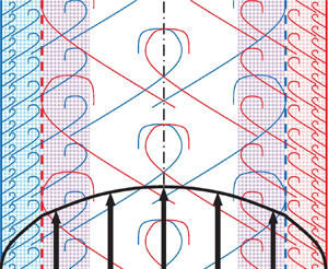
This hypothesis (2.1) is visualized by the cartoon of figure 3 and has two testable consequences:
(i) In pipe and channel flows the disturbances of opposite vorticity emanating from the opposite wall reduce
$\textrm {d} U^+/ \textrm {d} y^+$ for $y^+ > y^+_{{break}}$ and hence $\kappa > \kappa _{{M}}$. Conversely, in Couette flow these vorticity disturbances must increase the mean shear outside of $y^+_{{break}}$, leading to $\kappa < \kappa _{{M}}$.(ii) At sufficiently high
${Re}_{\tau }$, the short logarithmic layer with slope $(1/\kappa _{{M}})$ is possibly not influenced by geometry and the inner layer $0 \leq y^+ \leq y^+_{{break}}$ may therefore be universal, at least for the truly parallel flows considered here.


Figure 3. Cartoons illustrating the hypothesis 2.1. Red and blue shaded areas: wall layers not affected by the opposite wall; violet shade: overlap layers affected by ‘eddies’ originating from the opposite wall. (a) Overlap logarithmic slope reduced relative to the wall layers for pipe and channel flows; (b) overlap logarithmic slope increased relative to the wall layer for Couette flow.
Finding a theoretical underpinning for the above hypothesis or an alternative explanation is left for future research. For this, the variance of vorticity components in the simulations of Lee & Moser (Reference Lee and Moser2015) may provide a lead, as it changes from a  $1/y^+$ power-law decay to an exponential decay right around a
  $y^+$ of
  $10^3$, independently of
  ${Re}_{\tau }$.
2.3. Outline of §§ 3–5
In § 3, a number of high quality profiles for plane channel flow, up to  ${Re}_{\tau }=5186$ (Lee & Moser Reference Lee and Moser2015), are used to construct, for the first time, the complete inner and outer asymptotic expansions of
  $U^+$ up to terms of order
  ${O}({Re}^{-1}_{\tau })$. This allows the extraction of the leading-order MVP from DNS at low to moderate
  ${Re}_{\tau }$ values. In particular the leading-order inner profile
  $U^+_{{in, 0}}$, obtained in § 3.3, corroborates the hypothesis (2.1) by revealing a clean break point at
  $y^+_{{break}} \approxeq 600$, around which the logarithmic slope of
  $U^+$ decreases from (1/0.398) to (1/0.42) over a short
  $y^+$-distance.
An analogous reconstruction of 2-term asymptotic expansions from available Couette DNS, on the other hand, has not been feasible. Limited to the leading-order inner and outer asymptotic expansions, it is nevertheless possible to demonstrate in § 4.1, that the Couette DNS of Kraheberger, Hoyas & Oberlack (Reference Kraheberger, Hoyas and Oberlack2018) for  ${Re}_{\tau }=1026$ does show the steepening of
  $U^+$ at
  $y^+_{{break}}$, corresponding to
  $\kappa =0.367 < \kappa _{{\rm M}}=0.40$, in conformity with the hypothesis (2.1).
A brief review of three pipe DNS profiles in § 4.2 finally reveals, that the differences between available profiles are too large to attempt an analysis analogous to the one for the channel.
The paper closes with a recap of selected findings and a selection of open questions in § 5.
3. Higher-order asymptotic expansions of $U^+$ for the plane channel

At this point, the paper switches from phenomenology to a purely formal singular perturbation approach. The only assumptions for the following analysis are the restriction to the two classical inner and outer layers, connected through an overlap layer, which is at leading order of the physically motivated logarithmic form (1.1). However, no assumptions are made on the value of the Kármán parameter  $\kappa$, nor on the exact location of the overlap layer.
3.1. Methodology for extracting asymptotic expansions from DNS
The objective is to obtain, for the plane channel, the inner and outer asymptotic expansions of the mean velocity  $U^+$ up to and including the block order
  ${O}({Re}_{\tau }^{-1})$ (see Crighton & Leppington (Reference Crighton and Leppington1973), and § 1 for the concept of block order)
 \begin{equation} U^+_{{in}}(y^+) = U^+_{{in, 0}}(y^+) + {Re}_{\tau}^{{-}1} U^+_{{in, 1}}(y^+) + {O}( {Re}_{\tau}^{{-}2}), \end{equation}
and
 \begin{equation} U^+_{{out}}(Y) = U^+_{{out, 0}}(Y) + {Re}_{\tau}^{{-}1} U^+_{{out, 1}}(Y) + {O}( {Re}_{\tau}^{{-}2}),\end{equation}
together with the common part  $U^+_{{cp}}$, which can be expressed in terms of
  $y^+$,
  $Y$, or the intermediate variable
  $\eta =y^+{Re}_{\tau }^{-1/2}=Y{Re}_{\tau }^{1/2}$. Identifying the composite expansion
  $U^+_{{comp}}=U^+_{{in}}+U^+_{{out}}-U^+_{{cp}}$ with
  $U^+_{{DNS}}$, the first two orders in the expansions (3.1) and (3.2) are successively determined for the first time and fitted by suitable functions.
Rather counter-intuitively, the determination of the inner and outer expansions is best started with the order  ${O}({Re}^{-1}_{\tau })$ terms. Between the wall and the overlap region, the deviation of the inner velocity ((3.1)) from the total velocity, taken to be
  $U^+_{{DNS}}(y^+)$, is of the order of
  $\mid U^+_{{out}}(Y)-U^+_{{cp}}\mid$. Hence, assuming that the asymptotic expansion (3.1) converges rapidly (an assumption justified a posteriori), one obtains a good estimate of
  $U^+_{{in, 1}}(y^+)$ between the wall and the overlap layer by taking differences of two total velocity profiles at equal
  $y^+$ values (obtained by 3-point quadratic interpolation of the original DNS data) and different
  ${Re}_{\tau }$ values
 \begin{align} &[U^{+}_{{DNS}}(y^+;{Re}_{\tau, 1}) - U^{+}_{{DNS}}(y^+;{Re}_{\tau, 2})] [{Re}^{{-}1}_{\tau, 1} - {Re}^{{-}1}_{\tau, 2}]^{{-}1} \nonumber\\ &\quad =U^+_{{in},1}(y^+) + {O}( {Re}_{\tau}^{{-}1}; \mid U^+_{{out}}(Y) - U^+_{{cp}}\mid). \end{align}
 Similarly, between the overlap region and the centreline, the outer velocity ((3.2)) is equal to the total velocity  $U^+_{{DNS}}(Y)$, with an error of order
  $\mid U^+_{{in}}(y^+)-U^+_{{cp}}\mid$. However, obtaining the first-order term
  $U^+_{{out, 1}}(Y)$ is a bit trickier, because the leading block order of the outer expansion (3.2) is of the well-known form
 \begin{equation} U^+_{{out, 0}}(Y) = (1/\kappa) \ln( {Re}_{\tau}) + F(Y).\end{equation}
 Two strategies to determine  $U^+_{{out, 1}}(Y)$ are pursued in § 3.2:
(i) The first is to assume
$\kappa$ in (3.4) and to use the analogue of (3.3) to determine $U^+_{{out, 1}}(Y; \kappa )$. The ‘true’ $U^+_{{out, 1}}(Y)$ is then obtained by iterating on $\kappa$ until the best collapse of $U^+_{{out, 1}}(Y)$ is obtained from different profile pairs.(ii) The second, assumption-free strategy is to use a third DNS profile at a different Reynolds number to eliminate the
$(1/\kappa ) \ln ({Re}_{\tau })$ term from the two DNS profiles at ${Re}_{\tau , 1}$ and ${Re}_{\tau , 2}$, before proceeding analogous to (3.3).


The strategies outlined above to educe higher-order terms from DNS, are fundamentally different from the attempts to determine higher-order terms in the overlap region, discussed in § 1. Here,  $U^+_{{in, 1}}(y^+)$ and
  $U^+_{{out, 1}}(Y)$ are determined from the profiles in the inner wall region and the outer region near the centreline, respectively. Their proper matching in the overlap region only serves as an a posteriori verification.
The primary difficulty in implementing the above program is the required extraordinary fidelity of the DNS. Deviations from the Navier–Stokes solution must be sufficiently smaller than  $U^+/{Re}_{\tau }$ in order to extract the
  ${O}({Re}^{-1}_{\tau })$ terms with any kind of confidence, since profile uncertainties are amplified by a factor of the order of the smaller
  ${Re}_{\tau }$ used in (3.3). At first thought, one might wish for higher DNS Reynolds numbers in order to obtain a better separation of inner and outer scales and hence a clean(er) overlap log law. However, if the uncertainty of the DNS does not diminish at least as
  $1/{Re}_{\tau }$, nothing is gained for the determination of higher-order terms in the asymptotic expansion. In other words, it appears more important to improve the fidelity of DNS than to keep increasing the Reynolds number. Finally, it has to be kept in mind that the dependence of the
  $U^+$ profiles on additional parameters, such as the computational box size, has to be much weaker than its dependence on
  ${Re}_{\tau }$.
The four DNS profiles listed in table 1 have been found to produce consistent results for both first-order terms  $U^+_{{in, 1}}$ and
  $U^+_{{out, 1}}$ in the expansions (3.1) and (3.2), and will in the following be referred to by their profile number in the table. The principal computational characteristics of these DNS are summarized in table 1 of Lee & Moser (Reference Lee and Moser2015).
Table 1. Channel DNS profiles used to determine contributions of  ${O}({Re}_{\tau }^{-1})$.

3.2. The outer expansion $U^+_{{out}}(Y)$

The first-order outer profile  $U^+_{{out}, 1}(Y)$ is determined with both methods discussed in § 3.1. Iterating on
  $\kappa$, until the best collapse of
  $U^+_{{out}, 1}(Y; \kappa , i, j)$ determined from different profile pairs
  $(i,j)$ is obtained in the core of the channel, leads to
  $\kappa = 0.42$. The resulting good collapse in the region
  $0.4 \lesssim Y \leq 1$ of the
  $U^+_{{out}, 1}(Y)$, obtained from different pairs, is shown in figure 4(a), together with the fit
 \begin{equation} \hat{U}^+_{{out}, 1} ={-}210 - 130 \cos({\rm \pi} Y) \sim{-}340 + {O}(Y^2) \quad \mathrm{for}\quad Y\to 0, \end{equation}
where the reader is reminded that analytical fits are designated by hats, while quantities derived from DNS profiles are left without.

Figure 4. (a) Higher-order term  $U^+_{{out}, 1}(Y)$ of the outer expansion for the optimal
  $\kappa = 0.42$, obtained with pairs of DNS from table 1: —, (#1,#3); - - -, (#1,#4);
  $-\cdot -$, (#1,#2);
  $-\cdot \cdot -$, (#2,#3);
  $\bullet \bullet \bullet$ (magenta), fit by (3.5); grey:
  $U^+_{{out}, 1}(Y)$ with same profile pairs, but
  $\kappa = 0.41$. (b) Derivative
  $\textrm {d} U^+_{{out}, 1}(Y)/ \textrm {d} Y$ obtained from the same DNS pairs as in (a);
  $\bullet \bullet \bullet$ (magenta), derivative of (3.5).
As it turns out, the optimal  $\kappa = 0.42$ is rather sharply defined, as seen from the divergence of the
  $U^+_{{out}, 1}(Y)$ profiles for
  $\kappa =0.41$, obtained from the same profile pairs and included in figure 4(a) in grey. The confidence in the fit (3.5) is reinforced by the good match in figure 4(b) between the derivative of the fit (3.5) and the derivatives
  $\textrm {d} U^+_{{out}, 1}/ \textrm {d} Y$ obtained from the same profile pairs as in figure 4(a), with a scheme analogous to (3.3) that requires no knowledge of
  $\kappa$.
Since the determination of  $U^+_{{out}, 1}(Y)$ is a key step of the present analysis, which tests the limits of present DNS, it is useful to compare with the parameter-free method (ii), based on three DNS profiles and outlined in § 3.1. The resulting
  $U^+_{{out}, 1}(Y)$ is shown in figure 5(a) for four profile triplets and the corresponding
  $\kappa$ values are shown in panel (b). What is striking in this figure, are the surprisingly good results for the two triplets involving only profiles from table 1. The results for
  $\kappa$ in particular, which deviate on the centreline by less than
  $\pm 0.003$ from
  $0.42$, are outstanding. In contrast, the results from the two triplets including a profile of table 2 are rather useless for the present purpose. They have been included to show why the present methodology fails with a number of DNS profiles: as seen in figure 5, the two ‘bad’ triplets yield results consistent with the two ‘good’ ones up to around
  $Y \approx 0.2$, where they are of no interest for the outer expansion, and become erratic towards the centreline. This suggests an imbalance of computational effort between near-wall and core regions, which has been recognized and corrected by the Texas group during the computations for Lee & Moser (Reference Lee and Moser2015) (private communication of R. Moser and M.K. Lee).

Figure 5. (a) Higher-order term  $U^+_{{out}, 1}(Y)$ of the outer expansion obtained from three DNS of table 1: —, (#1,#2,#3); - - - (green), (#1,#2,#4). Results involving one DNS of table 2:
  $-\cdot -$ (grey), (#2,#3,#6);
  $-\cdot \cdot -$ (grey), (#2,#3,#5);
  $\bullet \bullet \bullet$ (magenta), fit by (3.5). (b)
  $\kappa$ from the same triplets as in panel (a);
  $\bullet \bullet \bullet$ (magenta),
  $\kappa = 0.42$.
Table 2. Channel DNS profiles used to validate the composite fit (3.17).

To complete the outer expansion, the leading-order term of  $U^+_{{out}}(Y)$ is split into several contributions
 \begin{equation} U^+_{{out}}(Y) = \left\{\frac{1}{0.42} \ln[{Re}_{\tau} Y (2-Y)] + C + W_0(Y)\right\} + \frac{1}{{Re}_{\tau}} U^+_{{out}, 1} + \cdots ,\end{equation}
where all the terms, including the outer log term, satisfy the channel symmetry  $U^+(Y)=U^+(2-Y)$. This requirement is rarely implemented in the literature, where the original decomposition of Coles (Reference Coles1956) into simple logarithm and ‘wake’ dominates. The only unknowns left in the outer expansion (3.6) are the constant
  $C$ and the ‘wake function’
  $W_0(Y)$ (note that
  $W_0$ is different from Coles’ wake function because of the symmetrized log term). Specifying
  $W_0(Y=1)=0$ in (3.6) leads to the 2-term expansion of the centreline velocity
 \begin{equation} \hat{U}^+_{{cl}} = \left\{\frac{1}{0.42} \ln( {Re}_{\tau}) + 6.22\right\} - \frac{80}{{Re}_{\tau}} + {O}( {Re}_{\tau}^{{-}2}),\end{equation}
with the optimal  $C=6.22$. Equation (3.7) is seen in figure 6 to reproduce the reference DNS data of table 1 with an error of less than
  $0.2\,\%$, which is marginally better than the leading-order fit by Monkewitz (Reference Monkewitz2017).

Figure 6. Various channel/duct centreline velocities minus  $\hat{U}^+_{cl}$ ((3.7)) versus
  ${Re}_{\tau }$.
  ${\blacksquare}$ (purple)
  ${\blacksquare}$ (sky blue)
  ${\blacksquare}$ (green)
  ${\blacksquare}$ (spring green), DNS of table 1;
  ${\blacklozenge}$ (grey), other DNS used in Monkewitz (Reference Monkewitz2017);
  $\times$, Schultz & Flack (Reference Schultz and Flack2013);
  $+$, Zanoun, Durst & Nagib (Reference Zanoun, Durst and Nagib2003).
  $\cdot - \cdot$ (red),
  $\pm 0.2\,\%$ of
  $\hat{U}^+_{cl}$.
  $\cdots$, slope corresponding to the Musker
  $\kappa _{M} =0.398$ ((3.16)).
Finally,  $W_0$ is obtained from (3.6) by using the fit (3.5) for
  $U^+_{{out}, 1}$ and identifying the total velocity
  $U^+_{{out}}$ with
  $U^+_{{DNS}}$ in the outer region. The resulting
  $W_0(Y)$ is shown in figure 7, together with its fit
 \begin{equation} \left.\begin{gathered} \displaystyle\dfrac{\textrm{d}\hat{W}_0}{\textrm{d} Y} = 2.66 \tanh\left\{3.66 \dfrac{1-Y}{[Y(2-Y)]^{2.5}}\right\}, \\ \displaystyle\hat{W}_0 ={-} \int_{Y}^{1} [ \textrm{d}\hat{W}_0/ \textrm{d} Y](Y') \,\textrm{d} Y' \sim{-}2.24 + 2.66 Y + {O}(Y^2) \quad \mathrm{for} \ Y\to 0,\end{gathered}\right\}\end{equation}
which is necessarily rather elaborate to avoid compromising the determination of the inner expansion in § 3.3. Note that the collapse of  $W_0$ from different DNS in figure 7 justifies the functional form of
  $U^+_{{out, 0}}$ in (3.6).


The two fits  $\hat {U}^+_{{out}, 1}$ and
  $\hat {W}_0$ complete the formal description of the 2-term outer expansion (3.6) of
  $U^+$. For the matching to the inner expansion, to be developed in § 3.3, the limiting behaviour of
  $\hat {U}^+_{{out}}$ for
  $Y\to 0$ is required. After expanding the logarithm in (3.6) and using the fits (3.5) and (3.8), one obtains for
  $Y \ll 1$
 \begin{equation} \hat{U}^+_{{out}}(Y \ll 1) \sim \frac{1}{0.42} \ln( {Re}_{\tau} Y) + 5.63 + 1.47 Y - \frac{340}{{Re}_{\tau}} + {O}( {Re}_{\tau}^{{-}2}),\end{equation}
where the log-law constant  $B=5.63$ is the result of
  $C=6.22$ minus
  $2.24$ ((3.8)) plus
  $\ln (2)/0.42$ from the Taylor expansion of the logarithm in (3.6).
The terms of (3.9) will appear in the common part, only if they have a counterpart in the limit  $y^+\gg 1$ of the inner expansion. As will be seen in § 3.3, this is the case for all the terms in (3.9).
Before moving on to the inner expansion, it is worthwhile to document in figure 8 the significant improvement in the description of the outer velocity profile, brought about by the  ${O}({Re}_{\tau }^{-1})$ correction (3.5). Panel (a) documents the improved collapse of the four profiles of table 1 in the central part of the channel. Panel (b) is a variation of figure 7(a) of Jiménez & Moser (Reference Jiménez and Moser2007), showing the ‘outer indicator function’ with the proper symmetry about the centreline. It clearly demonstrates the improved profile collapse brought about in the central part of the channel by subtracting the outer
  $O({Re}_{\tau }^{-1})$ contributions associated with
  $\hat {U}^+_{{out}, 1}$ ((3.5)) from the DNS data. The discussion of the indicator function near the wall, obtained by subtracting the inner
  ${O}(Re^{-1}_\tau)$ contributions from DNS, is deferred to figure 12.

Figure 8. (a) The effect of subtracting the fit  $\hat {U}^+_{{out}, 1}$ ((3.5)) from the four DNS profiles of table 1. (b) Solid lines, outer indicator function
  $Y(1-Y/2)(\textrm {d} U^+_{{DNS}}/ \textrm {d} Y)$ versus
  $Y$ for the three highest
  ${Re}_{\tau }$; corresponding
  $\bullet \bullet \bullet$, DNS minus first-order fit
  $Y(1-Y/2)(\textrm {d} \hat {U}^+_{{out}, 1}/ \textrm {d} Y) {Re}_{\tau }^{-1}$ ((3.5)); — (magenta), leading-order fit
  $Y(1-Y/2)(\textrm {d} \hat {U}^+_{{out}, 0}/ \textrm {d} Y)$ ((3.6) and (3.8)); - - - (magenta),
  $Y(1-Y/2)$ times derivative of logarithm in (3.6).
3.3. The inner expansion $U^+_{{in}}(y^+)$ and the final matching

Starting again with the order  ${O}({Re}_{\tau }^{-1})$, the first order of the inner expansion
  $U^+_{{in}, 1}(y^+)$ is determined with (3.3). Although at the limit of DNS uncertainty, different pairs of the profiles in table 1 yield reasonably consistent
  $U^+_{{in,1}}$, seen in figure 9 to have three distinct features:
(i) An initial negative excursion near the origin due to the pressure gradient, which produces the exact quadratic term
$-(\beta /2)(y^+)^2$ in the Taylor expansion of $U^+$ about the wall. This minute negative part is correctly reproduced by two of the four DNS pairs.(ii) A first-order ‘hump’ very similar to the hump proposed by Nagib & Chauhan (Reference Nagib and Chauhan2008) to improve the Musker profile (see appendix A and (A7)), except that its height diminishes as
${Re}_{\tau }^{-1}$.(iii) A final approach to the linear function
$1.47 y^+ - 340$ which matches the linear part of $\hat {U}^+_{{out}}(Y \ll 1)$ ((3.9)).


Figure 9. First-order term  $U^+_{{in}, 1}(y^+)$, obtained from differences (3.3) of
  $U^+$-profiles in table 1. Profile pairs and line styles as in figure 5(a) (green lines up to
  $Y=0.25$ for the lower
  ${Re}_{\tau }$ of the pair, grey lines beyond).
  $\bullet \bullet \bullet$ (magenta), complete fit
  $\hat {U}^+_{{in,1}}$ ((3.10)); - - - (magenta), linear function
  $1.47 y^+ - 340$ matching the linear part of
  $\hat {U}^+_{{out}}(Y \ll 1)$ ((3.9)). Inset: blowup of the origin with
  $\cdots$ (violet),
  $- (1/2) (y^+)^2$.
These three distinct features of the first-order inner velocity are fitted by the three terms of
 \begin{align} \hat{U}^+_{{in,1}} &={-}\tfrac{1}{2} (y^+)^2 \exp[{-}0.004(y^+)^3] + \hat{H}_{{NC}}(y^+; 67, 0.75, 27) \nonumber\\ &\quad + 490.5 \ln\cosh[2.996 10^{{-}3}y^+] \sim 1.47 y^+{-} 340 \quad \mathrm{for} \quad y^+\to \infty , \end{align}
with  $\hat {H}_{{NC}}$ the ‘hump’ function (A7). As required, the large
  $y^+$ limit of
  $\hat {U}^+_{{in,1}}/{Re}_{\tau }$ matches the corresponding terms in the small
  $Y$ expansion (3.9) of
  $\hat {U}^+_{{out}}$. Hence, the common part of the 2-term inner and outer expansions is
 \begin{equation} \hat{U}^+_{{cp}}(Y) = \left\{\frac{1}{0.42} \ln( {Re}_{\tau} Y) + 5.63 + 1.47 Y\right\} - \frac{340}{{Re}_{\tau}} + {O}( {Re}_{\tau}^{{-}2}) ,\end{equation}
or equivalently
 \begin{equation} \hat{U}^+_{{cp}}(y^+) = \left\{\frac{1}{0.42} \ln(y+) + 5.63\right\} +\frac{1}{{Re}_{\tau}} \{1.47 y^+{-} 340\} + {O}( {Re}_{\tau}^{{-}2}).\end{equation}
 The leading term  $U^+_{{in,0}}$ of the inner expansion is now finally obtained by identifying the 2-term composite expansion with the DNS profile
 \begin{equation} U^+_{{DNS}} \cong U^+_{{in,0}} + \hat{U}^+_{{out,0}} - \hat{U}^+_{{cp,0}}(y^+) + \frac{1}{{Re}_{\tau}}\left\{\hat{U}^+_{{in,1}} + \hat{U}^+_{{out,1}} - \hat{U}^+_{{cp,1}}(y^+)\right\}, \end{equation}
with the common part expressed in terms of  $y^+$, i.e. split into leading- and first-order parts according to (3.12). The resulting
  $U^+_{{in,0}}$ minus the leading-order common part is shown on the left axis of figure 10. For comparison, the same quantity, obtained without the
  ${O}({Re}_{\tau }^{-1})$ terms in (3.13), is plotted on the right axis and the striking improvement brought about by taking
  ${O}({Re}_{\tau }^{-1})$ terms into account is evident. This improvement also reveals a clean logarithmic region of
  $U^+_{{in,0}}$ beyond
  $y^+\approx 150$, where the Musker fit has already reached its design logarithmic asymptote with
  $\kappa _{{M}}=0.398$ and
  $B_{{M}}=4.717$. This first logarithmic region ends at a breakpoint
  $y^+_{{break}}=624$ (the magenta circle in figure 10), where
  $U^+_{{in,0}}$ switches to the true leading-order overlap log law
  $(1/0.42) \ln (y^+) + 5.63$ of (3.12).

Figure 10. Left axis and solid lines: leading-order inner velocity  $U^+_{{in, 0}}$ minus
  $U^+_{{cp, 0}}(y^+)$ obtained from (3.13) and (3.12) for the four profiles of table 1. Right axis and broken lines: leading-order inner velocity minus common part, equal to
  $U^+_{{DNS}} - \hat {U}^+_{{out,0}}$, determined without the
  ${O}({Re}_{\tau }^{-1})$ terms in (3.13).
  $\cdots$ (lime green), improved Musker profile
  $\hat {U}^+_{{mM}}$ ((A6)) without ‘hump’, for
  $\kappa _{{M}}=0.398$ and
  $B_{{M}}=4.784$, minus
  $\hat {U}^+_{{cp},0}(y^+)$ ((3.12));
  $\cdots$ (magenta),
  $\hat {U}^+_{{mM}}-\hat {U}^+_{{cp},0}(y^+) - \hat {\varDelta }_{{\log ,Ch}}$, including the change in logarithmic slope ((3.14)) at
  ${\bigcirc}$ (magenta), the breakpoint
  $y^+_{{break}}=624$.
This change of logarithmic slope at  $y^+_{{break}}=624$ is well fitted by the function
 \begin{equation} \hat{\varDelta}_{{\log,Ch}}(y^+) = \frac{1}{4} \left[\frac{1}{0.398} - \frac{1}{0.42}\right] \ln\left[1 + \left(\frac{y^+}{624}\right)^4\right],\end{equation}
already used by Monkewitz (Reference Monkewitz2017).
The last term of the 2-term composite expansion of  $U^+$ to be fitted is
  $U^+_{{in, 0}}$. This is achieved in two steps. First, the modified Musker profile ((A6)) with
  $\kappa _{{M}}=0.398$ and
  $B_{{M}}=4.784$ is subtracted, and the changeover to the true log law
  $\hat {\varDelta }^+_{{\log , ch}}$ ((3.14)) is added. The result is shown in figure 11(a) which reveals the leading-order hump, seen to be similar to the one discussed by Nagib & Chauhan (Reference Nagib and Chauhan2008). To maintain the highest possible fidelity of the fits, the hump of figure 11(a) is described by the modified Hump function
 \begin{equation} \hat{H}_{{mNC}}(y^+) = \hat{H}_{{NC}}(y^+; 0.313, 1.3, 33) - 4 \times 10^{{-}5}(y^+)^4 \exp\left[-(0.12 y^+)^{2.5}\right], \end{equation}
with the function  $\hat {H}_{{NC}}$ given by (A7).

Figure 11. (a) Value of  $U^+_{{in, 0}} - \hat {U}^+_{{mM}} + \hat {\varDelta }_{{\log ,Ch}}$ ((A6) and (3.14)) for the four profiles of table 1 (colour scheme in table);
  $\bullet \bullet \bullet$ (magenta), fit by (3.10) (b) DNS profiles
  $U^+_{{DNS}}$ minus complete composite fit
  $\hat {U}^+_{{comp}}$ up to and including
  ${O}({Re}_{\tau }^{-1})$ terms; horizontal dashed lines indicate
  $\pm 0.02$ from the composite fit. (a,b): - - -, validation cases of table 2 (colour scheme of table).
Putting (A6), (3.14) and (3.15) together, the complete fit of  $U^+_{{in, 0}}$ is obtained as
 \begin{equation} \hat{U}^+_{{in, 0}} = \hat{U}^+_{{mM}}(y^+; 0.398, 4.784) - \hat{\varDelta}_{{\log,Ch}} + \hat{H}_{{mNC}}.\end{equation}
At this point, all the terms of the composite expansion have been fitted, and the complete 2-term composite fit
 \begin{equation} \hat{U}^+_{{comp}} \cong \hat{U}^+_{{in,0}} + \hat{U}^+_{{out,0}} - \hat{U}^+_{{cp,0}}(y^+) + \frac{1}{{Re}_{\tau}} \left\{\hat{U}^+_{{in,1}} + \hat{U}^+_{{out,1}} - \hat{U}^+_{{cp,1}}(y^+)\right\},\end{equation}
can now be compared to the four DNS profiles of table 1. The result is shown in figure 11(b) which demonstrates an unprecedented collapse of all the four DNS profiles onto the composite profile  $\hat {U}^+_{{comp}}$, with absolute deviations of less than
  $\pm 0.02$.
This is also the moment to validate the new 2-term composite MVP fit ((3.17)), obtained as the average from different combinations of the four DNS in table 1, by comparing to the two profiles from independent sources in table 2. As seen in figure 11, the validation profiles are within the band of variations between the four ‘Master’ profiles up to  $y^+ \approxeq 200$, but show deviations of the order of
  $0.1$ in the outer part. While this represents less than 0.5 % of the local
  $U^+$, it prevented the use of these profiles for the determination of
  $U^+_{{out, 1}}$ (see also figure 5).
As the implications of pushing the asymptotic expansion of  $U^+$ to order
  ${O}({Re}_{\tau }^{-1})$ and of the excellent data collapse in figure 11 may not be obvious, the indicator function
  $\varXi ^+=y^+(\textrm {d} U^+/ \textrm {d} y^+)$, commonly used to locate logarithmic regions, is examined next. Since the overlap log-law results from an asymptotic argument, it must correspond to a region where the leading-order indicator function is constant. With the present results it is, for the first time, possible to subtract the first-order contribution of
  ${O}({Re}_{\tau }^{-1})$ from the full indicator profiles, as shown in figure 12. The salient features of this figure are:
(i) The
$\varXi ^+_{{DNS}}$, obtained directly from DNS profiles, as well as the composite $\hat {\varXi }^+_{{comp}}$ at higher ${Re}_{\tau }$ are substantially different from the leading-order fit of the inner indicator function $\hat {\varXi }^+_{{in}, 0}$, obtained from (3.16). Here, and in the following, $\varXi ^+$ with a subscript indicates which term of the asymptotic expansion of $U^+$ is used. The large deviation of $\varXi ^+_{{DNS}}$ from the leading order is principally due to the third part of $\hat {U}^+_{{in,1}}$ ((3.10)), which becomes the linear term $1.47 y^+/{Re}_{\tau }$ in the common part (3.12). The contribution of the outer $\hat {\varXi }^+_{{out, 1}}$ ((3.5)) is shown in figure 12 only for ${Re}_{\tau }=10^3$ (profile #3 of table 1), as it becomes negligible in the overlap region for ${Re}_{\tau } \gtrsim 4000$.(ii) From the above it is obvious, that the emergent horizontal tangent of
$\varXi ^+_{{DNS}}$ in profile #1 of table 1 and #5 of table 2 is a transient feature for ${Re}_{\tau } \approx 5000$, not related to the true overlap plateau of the leading-order indicator function at $1/0.42$.(iii) The full indicator function
$\varXi ^+_{{DNS}}$ only reveals the true overlap plateau, i.e. the clean overlap log law with $\kappa =0.42$, well beyond a ${Re}_{\tau }$ of $10^5$. For ${Re}_{\tau } = 10^6$ this plateau extends from $y^+=10^3$ to $10^4$, or $Y=10^{-3}$ to $10^{-2}$, with the intermediate variable $y^+{Re}_{\tau }^{-1/2}={O}(1)$, as ‘in the textbook’. This means, that at the highest DNS ${Re}_{\tau }$ of 5186 it is not possible to obtain the true overlap $\kappa$ from the indicator function.(iv) Figure 12 finally shows, that subtracting the fit
$\hat {\varXi }^+_{{in}, 1}$ for the first-order inner indicator function from $\varXi ^+_{{DNS}}$ dramatically improves the situation: It produces a good collapse of all the data derived from DNS onto the leading order $\varXi ^+_{{DNS}}-\hat {\varXi }^+_{{in}, 1}$ and suggests that, by subtracting $\hat {\varXi }^+_{{in}, 1}$, the true overlap log law could be identified already at ${Re}_{\tau } \approxeq 2\times10^4$.


Figure 12. Solid lines, channel indicator function  $\varXi ^+_{{DNS}}$ versus
  $y^+$ for the three highest
  ${Re}_{\tau }$ of table 1 plus three profiles obtained from the 2-term composite expansion (3.17) for
  ${Re}_{\tau } = 2\times10^4, 10^5$ and
  $10^6$; short dashes - - -,
  $\varXi ^+_{{DNS}}$ of validation profiles in table 2 (colours as in table);
  $\bullet \bullet \bullet$, corresponding
  $\varXi ^+_{{DNS}}-\hat {\varXi }^+_{{in, 1}}$;
  $- \cdot -$ (spring green),
  $\varXi ^+_{{DNS}}-\hat {\varXi }^+_{{in, 1}}-\hat {\varXi }^+_{{out, 1}}$ for profile #3 of table 1.
  $- - -$ (magenta), leading-order inner fit
  $\hat {\varXi }^+_{{in, 0}}$ (obtained from (3.16));
  $- \cdot \cdot -$ (purple), transitory plateau
  $1/0.384$ in
  $\varXi ^+_{{DNS}}$ for profile #1 of table 1.
It is also worthwhile to compare the Reynolds stress from DNS to the fit obtained from the momentum equation and the derivative of the 2-term composite expansion (3.17). The result is shown in figure 13 for four  ${Re}_{\tau }$. For
  ${Re}_{\tau }=5186$ the composite expansion is seen to match the DNS #1 of table 1 within plotting accuracy, as expected from the quality of the fit for
  $U^+$, shown in figure 11(b). Also included in figure 13 are the locations and values of the Reynolds stress maxima. As the maximum results from a balance between derivatives of inner and outer
  $U^+$, its location scales on the intermediate variable
  $\eta =y^+{Re}_{\tau }^{-1/2}=Y{Re}_{\tau }^{1/2}$, as recognized by Sreenivasan & Sahay (Reference Sreenivasan and Sahay1997). Hence, for sufficiently high
  ${Re}_{\tau }$, the Reynolds stress maximum must be located within the logarithmic common part of inner and outer expansions
 \begin{equation} y^+_{{maxRS}} = \left(\frac{{Re}_{\tau}}{\kappa}\right)^{1/2}+{O}( {Re}_{\tau}^{{-}1/2}), \quad 1 + \langle uv\rangle^+_{{max}} = \frac{2}{(\kappa {Re}_{\tau})^{1/2}}+ {O}( {Re}_{\tau}^{{-}1}).\end{equation}
This leading-order result, stated already by Lee & Moser (Reference Lee and Moser2015), with  $\kappa = 0.42$ is seen in figure 13 to closely match even the DNS for
  ${Re}_{\tau }=5186$, despite
  $y^+_{{maxRS}}$ being still well below the start of the overlap layer at
  $y^+_{{break}}=624$. Equation (3.18a,b) with
  $\kappa = 0.42$ yields
  $1+\langle uv\rangle ^+_{{max}}=3.09/{Re}_{\tau }^{1/2}$, which is within 0.3 % of the correlation of Sreenivasan & Sahay, but the location
  $y^+_{{maxRS}}=1.54 {Re}_{\tau }^{1/2}$ is slightly below the range of
  $1.6-2 {Re}_{\tau }^{1/2}$ in their figure 2. Note, however, that Sreenivasan & Sahay (Reference Sreenivasan and Sahay1997) implicitly assumed the same
  $\kappa$ for channel and pipe, which is not justified in view of the present findings.

Figure 13. Solid lines,  $1+\langle uv\rangle ^+$ obtained from the momentum equation and the 2-term composite expansion of
  $\hat {U}^+$, for
  ${Re}_{\tau } = 5186, 2\times10^4, 10^5$ and
  $10^6$; - - - (red),
  ${Re}_{\tau } = \infty$; small white
  $\circ$, 1 minus computed Reynolds stress from DNS #1 in table 1.
  $\bullet$, value and location of maximum Reynolds stress ((3.18a,b)) for the four
  $Re_\tau$, with
  $\kappa = 0.42$; white
  $\Diamond$, maximum Reynolds stress from DNS #1;
  $- \cdot -$ (green), Taylor expansion
  $1 - 0.00125(y^+)^3 + \cdots$ around
  $y^+=0$.
Finally, it is interesting to note that the leading term  $0.00125(y^+)^3$ of the Taylor expansion of the fitted Reynolds stress around
  $y^+=0$ is, within the uncertainty, identical to
  $0.00127(y^+)^3$ estimated by Monkewitz & Nagib (Reference Monkewitz and Nagib2015) from DNS of ZPG TBLs.
In conclusion, this analysis has, for the first time, uncovered the true asymptotic channel MVP, which is, at the  ${Re}_{\tau }$ of current DNS, hidden ‘under’ the inner and outer finite Reynolds number corrections. In particular, it has shown, that there is a statistically significant difference between the near-wall Musker
  $\kappa _{{M}}$ and the overlap
  $\kappa$ (see figure 12). In other words, the asymptotic structures of channel and Superpipe MVPs are similar, as seen in figure 14.

Figure 14. (a) Channel mean velocity profiles minus the leading-order common part  $\hat {U}^+_{{cp, 0}}=(1/0.42)\ln (y^+)+5.63$ ((3.12)). DNS profiles from tables 1 and 2 plus composite profiles for
  ${Re}_{\tau } = 2\times10^4, 10^5$ and
  $10^6$ ((3.17)), with same colour scheme as in figure 12. - - - (magenta), modified Musker profile
  $\hat {U}^+_{{mM}}(y^+; 0.398, 4.78)$ ((A6)) plus ‘hump’
  $\hat {H}_{{mNC}}$ ((3.15)) minus
  $\hat {U}^+_{{cp, 0}}$.
  $- \cdot -$,
  $\hat {U}^+_{{cl, 0}} - \hat {U}^+_{{cp, 0}} = 0.59$. (b) Analogous graph for the Superpipe profiles of Zagarola & Smits (Reference Zagarola and Smits1998) at comparable
  ${Re}_{\tau }$ values of
  $1.09, 2.35, 5.02, 19.7, 102, 529 \times 10^3$ minus the common part
  $\hat {U}^+_{{cp, 0}}=(1/0.436)\ln (y^+)+6.20$. - - - (magenta), Musker profile
  $\hat {U}^+_{{M}}(y^+; 0.384, 4.26)+\hat {H}_{{NC}}(y^+; 0.351, 1, 30)$ ((A1) and (A7)) minus
  $\hat {U}^+_{{cp, 0}}$. Change of log slope (intersection of Musker asymptote and
  $\hat {U}^+_{{cp, 0}}$) at
  $y^+_{{break}}=450$.
  $- \cdot -$ ,
  $\hat {U}^+_{{cl}} - \hat {U}^+_{{cp}} = 1.45$, corresponding to
  $\hat {U}^+_{{cl}}$ of figure 1(b).
4. Evidence for the hypothesis (2.1) in Couette flow and review of pipe DNS
4.1. Couette flow
The main test of the hypothesis (2.1) consists of the demonstration, that in Couette flow the logarithmic slope of  $U^+$ increases at
  $y^+_{{break}}$. In terms of an ‘eddy’ model, this increase of logarithmic slope in the region
  $y^+\geq y^+_{{break}}$ is brought about by eddies, which originate from the opposite wall, evolve and weaken progressively, and finally stop contributing to the mean shear at
  $y^+_{{break}}$. It would be desirable to construct inner and outer asymptotic expansions to order
  ${O}({Re}^{-1}_{\tau })$ analogous to those for the channel in § 3. However, as seen in figure 15, the available DNS are limited to
  ${Re}_{\tau }\lessapprox 10^3$ and there are doubts on whether the turbulence is fully developed below
  ${Re}_{\tau }$ of 500. Furthermore, several of the authors cited in the caption of figure 15 report, that even the MVP is sensitive to both the streamwise and spanwise sizes of the computational box.

Figure 15. Various Couette centreline velocities minus  $\hat {U}^+_{{cl}}$ ((4.1)) versus
  ${Re}_{\tau }$ from different DNS.
  $\circ$, Tsukahara, Kawamura & Shingai (Reference Tsukahara, Kawamura and Shingai2006);
  ${\blacksquare}$ (Blue), Lee & Moser (Reference Lee and Moser2018);
  $\blacktriangle$ (orange), Avsarkisov et al. (Reference Avsarkisov, Hoyas, Oberlack and García-Galache2014);
  ${\blacklozenge}$ (green), Pirozzoli, Bernardini & Orlandi (Reference Pirozzoli, Bernardini and Orlandi2014);
  $\bullet$ (red), Kraheberger et al. (Reference Kraheberger, Hoyas and Oberlack2018). - - -,
  $(1/0.384)\ln ({Re}_{\tau })+3.75$ minus (4.1);
  $\cdots$,
  $(1/0.481)\ln ({Re}_{\tau })+7.01$ minus (4.1).
Therefore, only the most recent profile of Kraheberger et al. (Reference Kraheberger, Hoyas and Oberlack2018) for the highest  ${Re}_{\tau }=1026$, obtained with state of the art numerical methods, is analysed here. This, of course, limits the analysis to the leading order of inner and outer expansions and leaves some uncertainty about the coefficients of the expansions.
To start the analysis, the centreline  $\kappa$ and
  $C$ are determined from the data points of Lee & Moser (Reference Lee and Moser2018) at
  ${Re}_{\tau }=501$ and Kraheberger et al. (Reference Kraheberger, Hoyas and Oberlack2018) at
  ${Re}_{\tau }=1026$ in figure 15:
 \begin{equation} \hat{U}^+_{{cl}} = \tfrac{1}{0.367} \ln( {Re}_{\tau}) + 3.04.\end{equation}
Analogous to (3.6) for the channel, except for the opposite symmetry of the logarithm about the centreline, the leading-order outer velocity is described by
 \begin{gather} \hat{U}^+_{{out}}(Y) = \frac{1}{0.367} \ln\left[\frac{{Re}_{\tau} Y}{2-Y}\right] + 3.04 + W_0(Y) \quad \mathrm{with} \quad W_0(Y)= 2.15 \cos\left(\frac{\rm \pi}{2} Y\right), \end{gather}
 \begin{gather}\hat{U}^+_{{out}}(Y\ll 1) \sim \tfrac{1}{0.367} \ln( {Re}_{\tau} Y) + 3.30 + 1.36 Y + {O}(Y)^2. \end{gather}
Since the linear term in the small- $Y$ limit (4.3) translates in the inner expansion to a first-order term, not considered here, the common part consists of just the log law in (4.3):
 \begin{equation} \hat{U}^+_{{cp}} = \tfrac{1}{0.367} \ln(y^+) + 3.30.\end{equation}
 The simple wake function  $W_0(Y)$ of (4.2) is seen in panel (a) of figure 16 to provide an excellent fit to the DNS for
  $Y \gtrapprox 0.4$, which is all that can be expected at this low Reynolds number. Panel (b) of figure 16 shows the same
  $U^+_{{DNS}}(y^+)$ minus the outer fit
  $\hat {U}^+_{{out}}$ (equation (4.2)), which is equal to
  $\hat {U}^+_{{in}}-\hat {U}^+_{{cp}}$, up to terms of order
  ${O}({Re}^{-1}_{\tau })$. Fitting
  $\hat {U}^+_{{in}}$ with the modified Musker profile plus hump,
  $\hat {U}^+_{{mM}}(y^+; 0.367, 3.30) + \hat {H}_{{NC}}(y^+; 0.38, 1, 34)$ ((A6) and (A7) with the overlap parameters of (4.4)), is seen in figure 16(b) to be obviously inadequate. A proper fit of
  $U^+_{{in}}$ is only possible with
  $\kappa _{M}=0.40$, requiring a change of logarithmic slope at
  $y^+_{{break}}=379$, described by the function
 \begin{equation} \hat{\varDelta}_{{\log,Cou}}(y^+) = \frac{1}{4}\left[\frac{1}{0.40} - \frac{1}{0.367}\right] \ln\left[1 + \left(\frac{y^+}{379}\right)^4\right],\end{equation}
similar to  $\hat {\varDelta }_{{\log ,Ch}}$ of (3.14).

Figure 16. (a) — (green), Difference between the  $U^+$-profile of Kraheberger et al. (Reference Kraheberger, Hoyas and Oberlack2018) for
  ${Re}_{\tau } =1026$ and
  $\hat {U}^+_{{cp}}$ ((4.4));
  $\bullet \bullet \bullet$ (magenta), outer fit
  $\hat {U}^+_{{out}}(Y)$ ((4.2)) minus
  $\hat {U}^+_{{cp}}$ ((4.4)). (b) — (green),
  $U^+_{{DNS}}(y^+)$ minus the outer fit
  $\hat {U}^+_{{out}}$ ((4.2)); - - - (aquamarine),
  $\hat {U}^+_{{mM}}(y^+; 0.367, 3.30) + \hat {H}_{{NC}}(y^+; 0.38, 1, 34)$ ((A6) and (A7));
  $\bullet \bullet \bullet$ (magenta),
  $\hat {U}^+_{{in}} - \hat {U}^+_{{cp}}$ ((4.6) and (4.4)); - - -, asymptote of
  $\hat {U}^+_{{mM}}(y^+; 0.40, 4.64)$. (c) — (green),
  $U^+_{{DNS}}(y^+)$ minus the composite fit
  $\hat {U}^+_{{in}} + \hat {U}^+_{{out}} - \hat {U}^+_{{cp}}$.
Hence, the leading order of the inner expansion for the mean velocity in Couette flow is
 \begin{equation} \hat{U}^+_{{in}} = \hat{U}^+_{{mM}}(y^+; 0.40, 4.64) + \hat{H}_{{NC}}(y^+; 0.38, 1, 34) - \hat{\varDelta}_{{\log,Cou}}(y^+),\end{equation}
with the different terms given by (A6), (A7) and (4.5), respectively. The final composite profile is obtained by combining equations (4.2), (4.4) and (4.6). The result is seen in figure 16(c) to provide an excellent description of the DNS profile of Kraheberger et al. (Reference Kraheberger, Hoyas and Oberlack2018), except for the ‘wiggle’ between  $y^+ \approx 2$ and 70, which is due to the simple hump model of (A7). No attempt has been made to improve the hump fit as for the channel, because the central point, the demonstration of a switch from a lower (1/0.40) to a higher (1/0.367) logarithmic slope at
  $y^+_{{break}}\approxeq 400$, is not affected.
4.2. The prospects of extracting asymptotic expansions from pipe DNS
Of the three flows considered in this paper, pipe flow is by far the one of largest practical interest and it would therefore be highly desirable to develop a complete asymptotic description of its MVP from DNS, analogous to the one for the channel in § 3.
However, the three DNS data points, included as red squares in figure 1, do not even provide a consistent fit for the centreline velocity. Looking at the lines  $\pm (10^3/{Re}_{\tau })$, added to the figure to guide the eye, it appears that the coefficient of
  ${Re}_{\tau }^{-1}$ on the centreline must be less than
  $10^3$. However, it is not clear from the present data, whether the higher-order correction is positive, negative or zero – clearly, more high accuracy DNS profiles in the
  ${Re}_{\tau }$ range of
  $10^3 - 5\times10^3$ are needed to clarify the situation.
To show the necessary improvements in order to perform an analysis analogous to the one in § 3 for the channel, the DNS profiles minus an example outer logarithmic part
 \begin{equation} W_0(Y) = U^+_{{DNS}} - \left\{\tfrac{1}{0.42} \ln[{Re}_{\tau} Y(2-Y)] + 6.84\right\},\end{equation}
are shown in figure 17 for the three pipe DNS of figure 1. Comparing to figure 7, it is obvious that the core region and in particular the handling of the coordinate singularity on the centreline require more attention, before an analysis analogous to § 3 can be envisioned. In conclusion, the extraction of asymptotic expansions from DNS (or experiment) analogous to the channel is not yet feasible, and one is left with considerable uncertainty about  $\kappa _{M}$,
  $y^+_{{break}}$ and
  $\kappa$ for the pipe.

Figure 17. Pipe analogue to figure 7 with  $W_0$ of (4.7), for the three pipe DNS of figure 1: — (lavender),
  ${Re}_{\tau }=999$, — (aquamarine),
  ${Re}_{\tau }=1142$ and — (green),
  ${Re}_{\tau }=2003$. —, - - -,
  $- \cdot -$, corresponding tentative linear fits with slopes 4.0, 4.9 and 3.3, respectively.
5. Conclusions
The present investigation, in particular the determination of the 2-term inner and outer asymptotic expansions for the channel, together with the Superpipe data and a detailed analysis of the leading-order asymptotic expansions for a Couette flow DNS, has uncovered a common feature of ducted parallel flows: a change of logarithmic slope of the mean velocity  $U^+(y^+)$ at a
  $y^+_{{break}}$ of the order
  ${O}(10^3)$. According to the hypothesis (2.1), the sign of this slope change depends on the flow symmetry, with a slope decrease in channel and pipe flows and an increase in Couette flow.
The evidence for this phenomenon is strong for channel flow, due to a consistent set of DNS, analysed in § 3, and a rigorous asymptotic analysis, which shows that the log law in the common part of inner and outer mean velocity expansions emerges in the MVP at a much higher  ${Re}_{\tau }$ than previously thought. For Couette flow, the analysis of the DNS profile at the highest available
  ${Re}_{\tau }$ supports the hypothesis (2.1), but more DNS for
  ${Re}_{\tau }$ in the range
  $10^3 - 5\times10^3$ are needed to confirm the present findings and reduce the parameter uncertainty. For pipe flow, finally, the late start of the logarithmic overlap layer has been firmly established by the Superpipe and CICLoPE experiments, but the available DNS data base does not yet allow an analogous asymptotic analysis to narrow down the estimates of
  $\kappa _{M}$,
  $\kappa$ and
  $y^+_{{break}}$, obtained from the experiments.
The paper concludes with the following list of further observations and open questions:
(i) The analysis of both channel flow in § 3 and Couette flow in § 4.1, found for the logarithmic asymptote of the Musker profile beyond
$y^+\approxeq 150$ a $\kappa _{M}$ of close to 2/5. In the pipe, on the other hand, the different MVP fits require a $\kappa _{M}$ closer to the ZPG TBL value of 0.384. So the question, whether $\kappa _{M}$ for truly one-dimensional flows is universal or not, will have to wait for more high quality pipe and Couette DNS, which allow the extraction of reliable asymptotic expansions. The reader is reminded here, that the logarithmic asymptote of the Musker profile with slope $1/\kappa _{M}$ cannot belong to the overlap layer, i.e. the common part of inner and outer expansions, because the outer expansion does not contain the corner and the logarithmic region with slope $1/\kappa _{M}$ towards the wall.(ii) Once the overlap
$\kappa$ values for pipe and Couette flows are finally ‘nailed down’ with an uncertainty below say $\pm 0.005$, one should be able to answer the question, whether $\kappa$ is a function of the pressure gradient (see Nagib & Chauhan Reference Nagib and Chauhan2008 for the relation $\kappa (\beta )$ in TBLs), or rather depends on the symmetry $S$ of mean vorticity about the centreline, with $S=-1$ for channel and pipe, and $S=1$ for Couette flow and/or the duct geometry. In this paper, the change of logarithmic slope $(\kappa ^{-1} - \kappa _{M}^{-1})$ at $y^+_{{break}}$ has been determined as $-0.13$ for channels and $+0.22$ for Couette flow. As the $+0.22$ in § 4.1 may be on the high side (see figure 15), a relation such as $(\kappa ^{-1} - \kappa _{M}^{-1}) \approxeq 0.13 S$ appears possible for channel and Couette flows. However, there is a significant difference between channel and pipe, where $(\kappa ^{-1} - \kappa _{M}^{-1})$ is estimated at $\approxeq -0.3$, but could be as low as $-0.23$ based on McKeon et al. (Reference McKeon, Li, Jiang, Morrison and Smits2004) – see next point.(iii) From the present profile analyses, the approximate doubling of
$(\kappa ^{-1} - \kappa _{M}^{-1})$ from channel to pipe appears significant and may possibly be explained by taking the hypothesis (2.1) one step further, and also consider a dependence of $(\kappa ^{-1} - \kappa _{M}^{-1})$ on the geometry of the opposite wall. In channel and Couette flows the latter is flat, while its transverse curvature in the pipe could have a focussing effect for perturbations traversing the core. This explanation may be somewhat simplistic and does not take into account probable differences between vortical perturbations in channels and pipes, but cannot be ruled out either.(iv) The height of the ‘hump’ above the Musker profile ((A7)) around
$y^+$ of 30 is clearly dependent on ${Re}_{\tau }$, as shown in § 3 for channel flow. The maximum overshoot over the logarithmic Musker asymptote $\kappa _{M}^{-1}\ln (y^+)+B_{M}$ is approximately $0.19 + (65/{Re}_{\tau })$, which resolves the discrepancies between the height originally proposed by Nagib & Chauhan (Reference Nagib and Chauhan2008) and the fits of low Reynolds number data by Luchini (Reference Luchini2018).(v) As discussed in § 1, the linear term
$\lambda Y$ in the small-$Y$ limit of $U^+_{{out,0}}$, the leading order of the outer expansion, appears in the common part only if the inner expansion is carried to ${O}(Re^{-1}_\tau)$, i.e. contains a matching term $\lambda y^+/{Re}_{\tau }$ in the limit $y^+\to \infty$. Most recently, Luchini (Reference Luchini2017) has claimed that $\lambda$ is equal to the pressure gradient parameter $\beta$, which is equal to 0, 1 and 2 for Couette, channel and pipe flow, respectively. From the present profile analyses, $\lambda =1.36$ for Couette flow ((4.3)), $\lambda =1.47$ for channel flow ((3.9)) and $\lambda \in [2.1, 3.7]$ for pipe flow, where these latter values correspond to the range of estimated slopes of the three $W_0$ profiles in figure 17, minus $(2\kappa )^{-1}$ from the small-$Y$ expansion of $\kappa ^{-1}\ln (2-Y)$ (equation (4.7)). The reason for this discrepancy is exposed in appendix B.(vi) The sudden decrease of logarithmic slope at
$y^+_{{break}}\approxeq 600$, found in § 3.3 for the channel mean velocity $U^+$, appears also in the profiles of fluctuating pressure $\langle p'p'\rangle ^+$ obtained by Panton, Lee & Moser (Reference Panton, Lee and Moser2017). This is particularly evident for the pressure derived from the ${Re}_{\tau }=5186$ DNS data of Lee & Moser (Reference Lee and Moser2015) (profile #1 in table 1): in figure 1(a) of Panton et al. for the total $\langle p'p'\rangle ^+$, the decrease of slope from the interval $y^+\in [150, 600]$ to $y^+>600$ is perceptible, but not very marked. However, in their figure 3 the pressure indicator function for the highest ${Re}_{\tau }=5186$ clearly shows two plateaus with a decrease of logarithmic slope by around 5 % between $y^+$ of 500 and $10^3$. This slope change is also evident in their figure 4(a) for the ‘rapid pressure’. As noted by Panton et al. (Reference Panton, Lee and Moser2017), the near correspondence between the logarithmic slopes in the $\langle p'p'\rangle ^+$ profiles for the channel and the ones obtained in § 3 from the asymptotic analysis of $U^+$ is unexplained and begs for further research.(vii) The idea has been advanced by Hultmark et al. (Reference Hultmark, Vallikivi, Bailey and Smits2012) and Marusic et al. (Reference Marusic, Monty, Hultmark and Smits2013), that the identification of logarithmic regions is facilitated by looking for simultaneous log regions in the MVP and in second order statistics, in particular in
$\langle uu\rangle ^+$. It has been supported mainly by measurements in the Princeton Superpipe with the NSTAP miniature hot-wires. However, the significant difference between the Pitot and the NSTAP Superpipe MVPs (see Monkewitz (Reference Monkewitz2017), figure 6) have, to this author's knowledge, not been resolved. At lower ${Re}_{\tau }$, the second-order statistics do not appear more promising than the MVP to identify log regions, as evidenced by the indicator functions in Lee & Moser (Reference Lee and Moser2015, § 3.2) for the channel, where only the spanwise normal stress exhibits a short log region for $y^+$ between approximately 100 and 300. One may therefore consider the construction of multi-term asymptotic expansions for the second-order statistics, analogous to § 3 for the channel MVP. In order to do this, one has to know the proper asymptotic sequence, but for $\langle uu\rangle ^+$, for instance, even the leading term is still being debated. While the ‘attached eddy model’ leads to an inner peak of $\langle uu\rangle ^+$ which increases indefinitely as $\ln ({Re}_{\tau })$, Monkewitz & Nagib (Reference Monkewitz and Nagib2015) have demonstrated with the help of the complete momentum equation, that this inner peak remains finite in the ZPG TBL (see also the discussion in Monkewitz, Nagib & Boulanger Reference Monkewitz, Nagib and Boulanger2017).(viii) Finally, it might also be interesting to determine the distribution and type of eddies attached to, or originating from the opposite wall, which preserve the logarithmic law in the overlap layer beyond
$y^+_{{break}}$ (for the attached eddy model, see e.g. Marusic & Monty (Reference Marusic and Monty2019) and references therein).


Acknowledgements
I am grateful to my partner for bearing with me while staring at graphs for days on end. Thanks also to R. Panton for pointing out the connections to the fluctuating pressure profiles and to H. Nagib, M. Giometto and an anonymous referee for all the helpful comments on the manuscript.
Declaration of interests
The author reports no conflict of interest.
Appendix A. The ‘Musker’ fit for the inner $U^+$-profile, with additions

The Musker profile (Musker Reference Musker1979) is obtained by integrating  $\mathrm{d}U^+_M/ \textrm {d} y^+ =[\kappa _{M} S + (y^+)^2]$
  $[\kappa _{M} S + (y^+)^2 + \kappa _{M} (y^+)^3]^{-1}$ analytically, where the subscript
  $M$ designates parameters used to generate the Musker fit. Note in particular, that
  $\kappa _{M}$ is not necessarily equal to the overlap
  $\kappa$. The two parameters
  $\kappa _{M}$ and
  $S$ determine the asymptotic behaviour of the Musker profile
  $\hat {U}^+_{{M}} \sim \ln(y^+)/\kappa _{M} + B_{{M}}$ but, as noted by Nagib & Chauhan (Reference Nagib and Chauhan2008), the straightforward integration is prone to numerical near-cancellations. The problem is avoided by recasting the result in the following form:
 \begin{align} &\hat{U}^+_{{M}}(y^+;
\kappa_{M}, B_{M}) = \varGamma_1 \ln\left(1 -
\frac{y^+}{g_1}\right) + \frac{\varGamma_2}{2} \ln\left(1 -
\frac{g_2 y^+}{g_3} + \frac{(y^+)^2}{g_3}\right)
\nonumber\\ &\quad +\frac{2\varGamma_3 +
\varGamma_2g_2}{g_4}\left[\arctan\left(\frac{2 y^+{-}
g_2}{g_4}\right) +
\arctan\left(\frac{g_2}{g_4}\right)\right],
\end{align}
\begin{align} &\hat{U}^+_{{M}}(y^+;
\kappa_{M}, B_{M}) = \varGamma_1 \ln\left(1 -
\frac{y^+}{g_1}\right) + \frac{\varGamma_2}{2} \ln\left(1 -
\frac{g_2 y^+}{g_3} + \frac{(y^+)^2}{g_3}\right)
\nonumber\\ &\quad +\frac{2\varGamma_3 +
\varGamma_2g_2}{g_4}\left[\arctan\left(\frac{2 y^+{-}
g_2}{g_4}\right) +
\arctan\left(\frac{g_2}{g_4}\right)\right],
\end{align}
with
 \begin{gather} s_{1,2} =
\left(-\frac{S}{2}\right)^{1/3}\left\{1 +
\frac{2}{S(3\kappa_{M})^3} \pm \left[1 + \frac{4}{S(3
\kappa_{M})^3} \right]^{1/2}\right\}^{1/3},
\end{gather}
\begin{gather} s_{1,2} =
\left(-\frac{S}{2}\right)^{1/3}\left\{1 +
\frac{2}{S(3\kappa_{M})^3} \pm \left[1 + \frac{4}{S(3
\kappa_{M})^3} \right]^{1/2}\right\}^{1/3},
\end{gather}
 \begin{gather}g_1=s_1+s_2-\frac{1}{3\kappa_{M}};\quad g_2={-}g_1-\frac{1}{\kappa_{M}};
\end{gather}
\begin{gather}g_1=s_1+s_2-\frac{1}{3\kappa_{M}};\quad g_2={-}g_1-\frac{1}{\kappa_{M}};
\end{gather}
 \begin{equation}
g_3=\frac{1}{4}\left(s_1+s_2+\frac{2}{3\kappa_{M}}\right)^2
+ \frac{3}{4}(s_1-s_2)^2;\quad g_4=(4g_3-g_2^2)^{1/2},
\end{equation}
\begin{equation}
g_3=\frac{1}{4}\left(s_1+s_2+\frac{2}{3\kappa_{M}}\right)^2
+ \frac{3}{4}(s_1-s_2)^2;\quad g_4=(4g_3-g_2^2)^{1/2},
\end{equation}
 \begin{equation}
\varGamma_1=\frac{S+\kappa_{M}^{{-}1}g_1^2}{g_1^2-g_1g_2+g_3};\quad
\varGamma_2=\frac{1}{\kappa_{M}}-\varGamma_1;\quad
\varGamma_3=\frac{g_3\varGamma_1-S}{g_1}.
\end{equation}
\begin{equation}
\varGamma_1=\frac{S+\kappa_{M}^{{-}1}g_1^2}{g_1^2-g_1g_2+g_3};\quad
\varGamma_2=\frac{1}{\kappa_{M}}-\varGamma_1;\quad
\varGamma_3=\frac{g_3\varGamma_1-S}{g_1}.
\end{equation}
The additive log-law constant  $B_{M}$ is the limit
  $y^+\to \infty$ of (A1)
 \begin{equation} B_{M} ={-}\varGamma_1 \ln({-}g_1) - \frac{\varGamma_2}{2} \ln(g_2) + \frac{2 \varGamma_3 + \varGamma_2 g_2}{g_4} \left[\frac{\rm \pi}{2} + \arctan\left(\frac{g_2}{g_4}\right)\right], \end{equation}
and its desired value is obtained by a simple iteration on  $S$.
$S$.
The basic Musker profile (A1) provides a good approximation to actual near-wall profiles with a logarithmic region at large  $y^+$, but it also has shortcomings. One of them is the slow asymptotic approach to the log-law as
  $\hat {U}^+_{{M}}\to \kappa _{M}^{-1}y^+ +B_{M}+\kappa _{M}^{-2}(y^+)^{-1}+{O}(y^+)^{-2}$. This defect is irrelevant when fitting experimental data, but is of concern for the higher-order asymptotic expansion of § 3. It is easily corrected by cancelling the
  $(y^+)^{-1}$ deviation of
  $\hat {U}^+_{{M}}$ from the log law at large
  $y^+$, resulting in the modified Musker profile
 \begin{equation} \hat{U}^+_{{mM}}(y^+; \kappa_{M}, B_{M}) = \hat{U}^+_{{M}}(y^+; \kappa_{M}, B_{M}) - (\kappa_{M}^2 y^+)^{{-}1} \exp({-}100/y^+). \end{equation}
As shown in figure 18, the effect is to ensure a clean log law for  $y^+$ beyond approximately 150.

Figure 18. Improvement of the Musker profile (A1): - - -, original  $\hat {U}^+_{{M}} - [\kappa _{M}^{-1}\ln (y^+)+B_{{M}}]$ for
  $\kappa _{M}=0.396$ and
  $B_{{M}}=4.717$ (
 $S=905.86$);
  $-\cdot -\cdot$, asymptotic approach of
  $\hat {U}^+_{{M}}$ to the log law; — (red), modified
  $\hat{U}^+_{mM}$ minus log law ((A6));
  $\cdot \cdot \cdot$ (red), corrective term in (A6).
Another, more prominent, defect of the basic Musker profile is that it is too low in a region around  $y^+$ of 30. This has first been described by Nagib & Chauhan (Reference Nagib and Chauhan2008), who added to the Musker profile the ‘hump’ function
 \begin{equation} \hat{H}_{{NC}}(y^+; h_1, h_2, h_3) = h_1 \exp[- h_2 \ln^2(y^+{/}h_3)], \end{equation}
with the original parameters  $h_1=0.351$,
  $h_2=1$ and
  $h_3=30$. Their addition of a higher-order term, behaving as
  $-0.5 \beta (y^+)^2/{Re}_{\tau }$ for
  $y^+\to 0$ with
  $\beta$ the pressure gradient parameter, is, however, not consistent, if the Musker profile is used as an approximation for the leading order of the inner asymptotic expansion of
  $U^+$.
Appendix B. Comment on the dimensional analysis of Luchini (Reference Luchini2017)
Luchini (Reference Luchini2017) (see also Luchini Reference Luchini2018) has used dimensional analysis to derive a higher-order linear pressure gradient correction of the log law. His analysis is briefly summarized here to pinpoint where it goes wrong.
Luchini's application of the Buckingham  $\varPi$ theorem starts with the five dimensional variables
  $\{(\textrm {d}\breve {U}/ \textrm {d}\breve {y}), \breve {y}, \breve {u}_\tau , (\partial \breve {p}/\partial \breve {x}), \breve {\rho } \}$. One immediately notes that this starting list of variables implicitly contains the hydraulic diameter
  $\breve {D}_H \equiv - 4 \breve {\tau }_w(\partial \breve {p}/\partial \breve {x})^{-1}$, while Luchini explicitly excluded the other outer length scale
  $\breve {L}$ (e.g. the channel half-height or pipe radius). From this starting list, two non-dimensional groupings are obtained,
 \begin{equation} \varPi_1 = \frac{\breve{y}(\textrm{d}\breve{U}/ \textrm{d}\breve{y})}{\breve{u}_{\tau}},\quad \varPi_2 ={-} \frac{\breve{y}(\partial\breve{p}/\partial\breve{x})}{\breve{\tau}_w} \equiv 4\frac{\breve{y}}{\breve{D}_H}, \end{equation}
which are related by the functional relation  $\varPi _1 = F(\varPi _2)$. Assuming that the function
  $F$ is analytic around
  $\varPi _2 = 0$, Luchini Taylor-expanded
  $F$ around
  $\varPi _2 = 0$ and truncated the series after the linear term
  $\propto \varPi _2$, which leads to (6) in Luchini (Reference Luchini2017) and, after non-dimensionalization and integration with respect to
  $y^+$, to
 \begin{equation} U^+{=} \kappa^{{-}1} \ln{y^+} + B + 4 A_1 \frac{y^+}{D_H^+}.\end{equation}
It is between (6) and (7) of Luchini (Reference Luchini2017) that the analysis goes wrong, when he replaces the single outer length scale  $D_H^+$ in the last term of (B2) by
  $\beta (4L^+)^{-1}$ and implies that
  $\beta = 4L^+/D_H^+$ and
  $L^+$ can be chosen independently, in contradiction with the exclusion of
  $\breve {L}$ from the list of starting variables for the Buckingham's
  $\varPi$ theorem. In other words, (7) of Luchini (Reference Luchini2017) is only valid for a fixed ratio of
  $D_H^+$ and
  $L^+ \equiv {Re}_{\tau }$, i.e. a fixed
  $\beta$.
Introducing also  $\breve {L}$ in the starting list of variables for the application of Buckingham's
  $\varPi$ theorem adds a third
  $\varPi _3 = \beta$ to the list of the parameters (B1). As a consequence, nothing prevents the three parameters
  $\kappa$,
  $B$ and
  $A_1$ in (B2) from becoming non-universal functions of
  $\beta$, as already suggested for
  $\kappa$ and
  $B$ by Nagib & Chauhan (Reference Nagib and Chauhan2008), Monkewitz (Reference Monkewitz2017) and Monkewitz (Reference Monkewitz2019), for instance.


 Open access