


1 Introduction
Relativistically intense (
 ${>}10^{18}~\text{W}\cdot \text{cm}^{-2}$
for a laser wavelength of
${>}10^{18}~\text{W}\cdot \text{cm}^{-2}$
for a laser wavelength of
 $\simeq 1~\unicode[STIX]{x03BC}\text{m}$
) laser–solid interactions provide a means to generate a compact source of highly energetic ions of ultrashort pulse duration[Reference Daido, Nishiuchi and Pirozhkov1, Reference Macchi, Borghesi and Passoni2]. The resultant ion beams can be used in a wide range of science and applications, including isochoric heating of matter[Reference Patel, Mackinnon, Key, Cowan, Foord, Allen, Price, Ruhl, Springer and Stephens3], ultrafast probing of transient electric and magnetic fields[Reference Borghesi, Campbell, Schiavi, Haines, Willi, MacKinnon, Patel, Gizzi, Galimberti, Clarke, Pegoraro, Ruhl and Bulanov4] and micron-scale proton radiography[Reference Mackinnon, Patel, Town, Edwards, Phillips, Lerner, Price, Hicks, Key, Hatchett and Wilks5]. There is also the potential to apply such beams to medical oncology[Reference Bulanov and Khoroshkov6] and fast-ignition inertial confinement fusion[Reference Roth, Cowan, Key, Hatchett, Brown, Fountain, Johnson, Pennington, Snavely, Wilks, Yasuike, Ruhl, Pegoraro, Bulanov, Campbell, Perry and Powell7]. The maximum energy, energy spread, beam parameter selectivity and beam spatial profile requirements for these potential applications drive the need to improve and optimize the underlying acceleration mechanisms.
$\simeq 1~\unicode[STIX]{x03BC}\text{m}$
) laser–solid interactions provide a means to generate a compact source of highly energetic ions of ultrashort pulse duration[Reference Daido, Nishiuchi and Pirozhkov1, Reference Macchi, Borghesi and Passoni2]. The resultant ion beams can be used in a wide range of science and applications, including isochoric heating of matter[Reference Patel, Mackinnon, Key, Cowan, Foord, Allen, Price, Ruhl, Springer and Stephens3], ultrafast probing of transient electric and magnetic fields[Reference Borghesi, Campbell, Schiavi, Haines, Willi, MacKinnon, Patel, Gizzi, Galimberti, Clarke, Pegoraro, Ruhl and Bulanov4] and micron-scale proton radiography[Reference Mackinnon, Patel, Town, Edwards, Phillips, Lerner, Price, Hicks, Key, Hatchett and Wilks5]. There is also the potential to apply such beams to medical oncology[Reference Bulanov and Khoroshkov6] and fast-ignition inertial confinement fusion[Reference Roth, Cowan, Key, Hatchett, Brown, Fountain, Johnson, Pennington, Snavely, Wilks, Yasuike, Ruhl, Pegoraro, Bulanov, Campbell, Perry and Powell7]. The maximum energy, energy spread, beam parameter selectivity and beam spatial profile requirements for these potential applications drive the need to improve and optimize the underlying acceleration mechanisms.
The most investigated laser-driven ion acceleration mechanism, target normal sheath acceleration (TNSA), occurs during intense laser pulse interactions with thin foil targets[Reference Wilks, Langdon, Cowan, Roth, Singh, Hatchett, Key, Pennington, MacKinnon and Snavely8]. The formation of an electric field with strength on the order of
 $\text{T}\,\cdot \,\text{V}\,\cdot \,\text{m}^{-1}$
at the target rear ionizes surface atoms and results in the acceleration of ions. This can produce ion beams with a smoothly varying Gaussian transverse profile in density and a thermal energy distribution[Reference Carroll, McKenna, Lundh, Lindau, Wahlström, Bandyopadhyay, Pepler, Neely, Kar, Simpson, Markey, Zepf, Bellei, Evans, Redaelli, Batani, Xu and Li9, Reference Wagner, Deppert, Brabetz, Fiala, Kleinschmidt, Poth, Schanz, Tebartz, Zielbauer, Roth, Stöhlker and Bagnoud10]. A promising alternative mechanism, known as radiation pressure acceleration (RPA)[Reference Esirkepov, Borghesi, Bulanov, Mourou and Tajima11], has received significant attention in recent years due to predicted favourable scaling of the maximum proton energy with intensity and the potential for the generation of monoenergetic spectra[Reference Robinson, Zepf, Kar, Evans and Bellei12]. In that case, the acceleration process begins at the front surface. The electrons at the front surface within the laser focal spot are collectively driven forward into the target when the intensity is high enough for the radiation pressure to exceed that of the plasma thermal pressure. This establishes a strong electric field that accelerates the ions. Depending upon the target thickness, hole-boring[Reference Robinson, Gibbon, Zepf, Kar, Evans and Bellei13, Reference Schlegel, Naumova, Tikhonchuk, Labaune, Sokolov and Mourou14] or light sail[Reference Esirkepov, Borghesi, Bulanov, Mourou and Tajima11] variations of this mechanism dominate and are predicted to result in peaked energy spectra[Reference Kar, Kakolee, Qiao, Macchi, Cerchez, Doria, Geissler, McKenna, Neely, Osterholz, Prasad, Quinn, Ramakrishna, Sarri, Willi, Yuan, Zepf and Borghesi15], higher energies, higher conversion efficiency and lower divergence compared with TNSA. The optimal target thickness for the light sail mode of RPA is typically determined to be on the order of tens of nanometres[Reference Macchi, Veghini and Pegoraro16] for currently achievable intensities. This mechanism can be susceptible to unstable behaviour at the critical surface[Reference Pegoraro and Bulanov17]. At such a thickness, the target can undergo relativistic self-induced transparency (RSIT)[Reference Tushentsov, Kim, Cattani, Anderson and Lisak18] where a combination of plasma heating to relativistic temperatures and plasma expansion results in the electron density reducing below the relativistically corrected critical density (
$\text{T}\,\cdot \,\text{V}\,\cdot \,\text{m}^{-1}$
at the target rear ionizes surface atoms and results in the acceleration of ions. This can produce ion beams with a smoothly varying Gaussian transverse profile in density and a thermal energy distribution[Reference Carroll, McKenna, Lundh, Lindau, Wahlström, Bandyopadhyay, Pepler, Neely, Kar, Simpson, Markey, Zepf, Bellei, Evans, Redaelli, Batani, Xu and Li9, Reference Wagner, Deppert, Brabetz, Fiala, Kleinschmidt, Poth, Schanz, Tebartz, Zielbauer, Roth, Stöhlker and Bagnoud10]. A promising alternative mechanism, known as radiation pressure acceleration (RPA)[Reference Esirkepov, Borghesi, Bulanov, Mourou and Tajima11], has received significant attention in recent years due to predicted favourable scaling of the maximum proton energy with intensity and the potential for the generation of monoenergetic spectra[Reference Robinson, Zepf, Kar, Evans and Bellei12]. In that case, the acceleration process begins at the front surface. The electrons at the front surface within the laser focal spot are collectively driven forward into the target when the intensity is high enough for the radiation pressure to exceed that of the plasma thermal pressure. This establishes a strong electric field that accelerates the ions. Depending upon the target thickness, hole-boring[Reference Robinson, Gibbon, Zepf, Kar, Evans and Bellei13, Reference Schlegel, Naumova, Tikhonchuk, Labaune, Sokolov and Mourou14] or light sail[Reference Esirkepov, Borghesi, Bulanov, Mourou and Tajima11] variations of this mechanism dominate and are predicted to result in peaked energy spectra[Reference Kar, Kakolee, Qiao, Macchi, Cerchez, Doria, Geissler, McKenna, Neely, Osterholz, Prasad, Quinn, Ramakrishna, Sarri, Willi, Yuan, Zepf and Borghesi15], higher energies, higher conversion efficiency and lower divergence compared with TNSA. The optimal target thickness for the light sail mode of RPA is typically determined to be on the order of tens of nanometres[Reference Macchi, Veghini and Pegoraro16] for currently achievable intensities. This mechanism can be susceptible to unstable behaviour at the critical surface[Reference Pegoraro and Bulanov17]. At such a thickness, the target can undergo relativistic self-induced transparency (RSIT)[Reference Tushentsov, Kim, Cattani, Anderson and Lisak18] where a combination of plasma heating to relativistic temperatures and plasma expansion results in the electron density reducing below the relativistically corrected critical density (
 $n_{\text{crit}}=\unicode[STIX]{x1D714}_{L}^{2}\unicode[STIX]{x1D716}_{0}\unicode[STIX]{x1D6FE}m_{e}/e^{2}$
where
$n_{\text{crit}}=\unicode[STIX]{x1D714}_{L}^{2}\unicode[STIX]{x1D716}_{0}\unicode[STIX]{x1D6FE}m_{e}/e^{2}$
where
 $\unicode[STIX]{x1D714}_{L}$
is the angular laser frequency,
$\unicode[STIX]{x1D714}_{L}$
is the angular laser frequency,
 $\unicode[STIX]{x1D716}_{0}$
the permittivity of free space,
$\unicode[STIX]{x1D716}_{0}$
the permittivity of free space,
 $\unicode[STIX]{x1D6FE}$
the electron Lorentz factor,
$\unicode[STIX]{x1D6FE}$
the electron Lorentz factor,
 $m_{e}$
the electron mass and –
$m_{e}$
the electron mass and –
 $e$
the electron charge). This enables the remainder of the laser pulse to be transmitted through the expanded target[Reference Vshivkov, Naumova, Pegoraro and Bulanov19]. With femtosecond laser pulses it has been observed that diffraction through the resultant plasma aperture can impact upon the particle dynamics[Reference Gonzalez-Izquierdo, Gray, King, Dance, Wilson, McCreadie, Butler, Capdessus, Hawkes, Green, Borghesi, Neely and McKenna20, Reference Gonzalez-Izquierdo, King, Gray, Wilson, Dance, Powell, Maclellan, McCreadie, Butler, Hawkes, Green, Murphy, Stockhausen, Carroll, Booth, Scott, Borghesi, Neely and McKenna21]. In the case of linearly polarized laser light, both the TNSA and RPA schemes can occur in a hybrid acceleration scenario[Reference Qiao, Kar, Geissler, Gibbon, Zepf and Borghesi22]. The onset of RSIT in this hybrid scenario has recently been shown experimentally to result in maximum proton energies close to 100 MeV for irradiation intensities of
$e$
the electron charge). This enables the remainder of the laser pulse to be transmitted through the expanded target[Reference Vshivkov, Naumova, Pegoraro and Bulanov19]. With femtosecond laser pulses it has been observed that diffraction through the resultant plasma aperture can impact upon the particle dynamics[Reference Gonzalez-Izquierdo, Gray, King, Dance, Wilson, McCreadie, Butler, Capdessus, Hawkes, Green, Borghesi, Neely and McKenna20, Reference Gonzalez-Izquierdo, King, Gray, Wilson, Dance, Powell, Maclellan, McCreadie, Butler, Hawkes, Green, Murphy, Stockhausen, Carroll, Booth, Scott, Borghesi, Neely and McKenna21]. In the case of linearly polarized laser light, both the TNSA and RPA schemes can occur in a hybrid acceleration scenario[Reference Qiao, Kar, Geissler, Gibbon, Zepf and Borghesi22]. The onset of RSIT in this hybrid scenario has recently been shown experimentally to result in maximum proton energies close to 100 MeV for irradiation intensities of
 ${\sim}3\times 10^{20}~\text{W}\cdot \text{cm}^{-2}$
[Reference Higginson, Gray, King, Dance, Williamson, Butler, Wilson, Capdessus, Armstrong, Green, Hawkes, Martin, Wei, Mirfayzi, Yuan, Kar, Borghesi, Clarke, Neely and McKenna23].
${\sim}3\times 10^{20}~\text{W}\cdot \text{cm}^{-2}$
[Reference Higginson, Gray, King, Dance, Williamson, Butler, Wilson, Capdessus, Armstrong, Green, Hawkes, Martin, Wei, Mirfayzi, Yuan, Kar, Borghesi, Clarke, Neely and McKenna23].
Studies have shown that, for ultrathin targets (
 ${\sim}5~\text{nm}$
), pressure perturbations produced at the laser–plasma interface during RPA can induce unstable wave behaviour associated with a Rayleigh–Taylor-like instability at the critical surface, where the density is equal to
${\sim}5~\text{nm}$
), pressure perturbations produced at the laser–plasma interface during RPA can induce unstable wave behaviour associated with a Rayleigh–Taylor-like instability at the critical surface, where the density is equal to
 $n_{\text{crit}}$
[Reference Pegoraro and Bulanov17, Reference Pegoraro and Bulanov24, Reference Sgattoni, Sinigardi, Fedeli, Pegoraro and Macchi25]. This can lead to filamentary structures in the RPA accelerated protons[Reference Palmer, Schreiber, Nagel, Dover, Bellei, Beg, Bott, Clarke, Dangor, Hassan, Hilz, Jung, Kneip, Mangles, Lancaster, Rehman, Robinson, Spindloe, Szerypo, Tatarakis, Yeung, Zepf and Najmudin26, Reference Powell, King, Gray, MacLellan, Gonzalez-Izquierdo, Stockhausen, Hicks, Dover, Rusby, Carroll, Padda, Torres, Kar, Clarke, Musgrave, Najmudin, Borghesi, Neely and McKenna27]. Simulations have indicated that the rippling of the laser–plasma interface dictates the spatial scale of this instability[Reference Sgattoni, Sinigardi, Fedeli, Pegoraro and Macchi25]. The use of elliptical polarization has been suggested to suppress this instability[Reference Wu, Zheng, Qiao, Zhou, Yan, Yu and He28]. For thicker targets, by generating a long-density scale length plasma at the rear surface, the counter-streaming of the fast electron population and the slower return current drawn from the denser background plasma to maintain current neutrality, can induce a Weibel instability[Reference Weibel29, Reference Morse and Nielson30] at the target rear surface. This results in the growth of transverse electromagnetic perturbations that form localized magnetic field structures that can grow to saturation[Reference Okada and Ogawa31]. This leads to filamentary structures in the background electron population which map into the TNSA-proton beam due to space-charge separation[Reference Scott, Brenner, Bagnoud, Clarke, Gonzalez-Izquierdo, Green, Heathcote, Powell, Rusby, Zielbauer, McKenna and Neely32]. Experiments using micron-scale diameter liquid hydrogen jets have also shown the development of the filamentary structures due to the Weibel instability near the critical density surface[Reference Göde, Rödel, Zeil, Mishra, Gauthier, Brack, Kluge, MacDonald, Metzkes, Obst, Rehwald, Ruyer, Schlenvoigt, Schumaker, Sommer, Cowan, Schramm, Glenzer and Fiuza33]. Ultrathin targets irradiated with intense laser will experience heating and expansion becoming sensitive to such instabilities. It is therefore vital to understand the factors that influence their onset and evolution.
$n_{\text{crit}}$
[Reference Pegoraro and Bulanov17, Reference Pegoraro and Bulanov24, Reference Sgattoni, Sinigardi, Fedeli, Pegoraro and Macchi25]. This can lead to filamentary structures in the RPA accelerated protons[Reference Palmer, Schreiber, Nagel, Dover, Bellei, Beg, Bott, Clarke, Dangor, Hassan, Hilz, Jung, Kneip, Mangles, Lancaster, Rehman, Robinson, Spindloe, Szerypo, Tatarakis, Yeung, Zepf and Najmudin26, Reference Powell, King, Gray, MacLellan, Gonzalez-Izquierdo, Stockhausen, Hicks, Dover, Rusby, Carroll, Padda, Torres, Kar, Clarke, Musgrave, Najmudin, Borghesi, Neely and McKenna27]. Simulations have indicated that the rippling of the laser–plasma interface dictates the spatial scale of this instability[Reference Sgattoni, Sinigardi, Fedeli, Pegoraro and Macchi25]. The use of elliptical polarization has been suggested to suppress this instability[Reference Wu, Zheng, Qiao, Zhou, Yan, Yu and He28]. For thicker targets, by generating a long-density scale length plasma at the rear surface, the counter-streaming of the fast electron population and the slower return current drawn from the denser background plasma to maintain current neutrality, can induce a Weibel instability[Reference Weibel29, Reference Morse and Nielson30] at the target rear surface. This results in the growth of transverse electromagnetic perturbations that form localized magnetic field structures that can grow to saturation[Reference Okada and Ogawa31]. This leads to filamentary structures in the background electron population which map into the TNSA-proton beam due to space-charge separation[Reference Scott, Brenner, Bagnoud, Clarke, Gonzalez-Izquierdo, Green, Heathcote, Powell, Rusby, Zielbauer, McKenna and Neely32]. Experiments using micron-scale diameter liquid hydrogen jets have also shown the development of the filamentary structures due to the Weibel instability near the critical density surface[Reference Göde, Rödel, Zeil, Mishra, Gauthier, Brack, Kluge, MacDonald, Metzkes, Obst, Rehwald, Ruyer, Schlenvoigt, Schumaker, Sommer, Cowan, Schramm, Glenzer and Fiuza33]. Ultrathin targets irradiated with intense laser will experience heating and expansion becoming sensitive to such instabilities. It is therefore vital to understand the factors that influence their onset and evolution.
In this article, we demonstrate for the first time that the degree of filamentary structure within a beam of protons accelerated due to the interaction of an intense laser pulse with an ultrathin target foil, is related to the extent of expansion of the rear surface proton layer, prior to the formation of magnetic field structures associated with the Weibel instability. Through the use of 2D particle-in-cell (PIC) simulations, the formation time of quasi-static azimuthal magnetic field structures is found to be related to both target expansion and fast electron propagation, both determined by the temporal laser intensity profile. At the same time, the TNSA mechanism occurs, causing the rear surface proton population to expand away from the forming magnetic field structures. This results in increased filamentary behaviour in the proton beam for the fastest magnetic field formation and least degree of proton layer expansion. These proton density structures are observed in both simulation and experiment, and are seen to vary when the laser intensity profile in time is modified via the use of two temporally separated laser pulses of differing intensities. This enables additional proton acceleration through RSIT mechanisms allowing these structures to be observed, while enabling the magnetic field formation and initial proton expansion to be varied at lower intensities. By understanding this interplay, we demonstrate fundamental insight into the sensitivity of laser-accelerated proton structures to the temporal laser intensity profile.

Figure 1. (a) Schematic illustrating of the relevant aspects of the experimental setup. The incoming laser pulse is reflected from a plasma mirror before irradiating the target at
 $30^{\circ }$
incidence with respect to the target normal. The spatial profile and energy of the beam of accelerated protons are measured using a radiochromic film stack at the rear of the target. (b) Schematic of the idealized temporal profile of the incoming laser pulse for varying
$30^{\circ }$
incidence with respect to the target normal. The spatial profile and energy of the beam of accelerated protons are measured using a radiochromic film stack at the rear of the target. (b) Schematic of the idealized temporal profile of the incoming laser pulse for varying
 ${\mathcal{E}}_{1}$
and
${\mathcal{E}}_{1}$
and
 ${\mathcal{E}}_{2}$
energies.
${\mathcal{E}}_{2}$
energies.
2 Experiment
The experiment was conducted by using the Vulcan petawatt laser at the Rutherford Appleton Laboratory. This laser delivered p-polarized pulses of light with a central wavelength of
 $1.053~\unicode[STIX]{x03BC}\text{m}$
focused with an
$1.053~\unicode[STIX]{x03BC}\text{m}$
focused with an
 $f/3$
off-axis parabolic mirror and reflected from a single planar plasma mirror[Reference Ziener, Foster, Divall, Hooker, Hutchinson, Langley and Neely34]. The focal spot diameter on the target solid was
$f/3$
off-axis parabolic mirror and reflected from a single planar plasma mirror[Reference Ziener, Foster, Divall, Hooker, Hutchinson, Langley and Neely34]. The focal spot diameter on the target solid was
 $7.3~\unicode[STIX]{x03BC}\text{m}$
(full width at half maximum (FWHM)). The targets were either thin aluminium, or plastic (CH) foils with thickness,
$7.3~\unicode[STIX]{x03BC}\text{m}$
(full width at half maximum (FWHM)). The targets were either thin aluminium, or plastic (CH) foils with thickness,
 $l$
, varied between 10 nm and 40 nm. A schematic of the experimental setup is shown in Figure 1(a). The on-target energy was
$l$
, varied between 10 nm and 40 nm. A schematic of the experimental setup is shown in Figure 1(a). The on-target energy was
 ${\mathcal{E}}_{0}=(200\pm 15)~\text{J}$
configured to provide either a single pulse, with a duration of
${\mathcal{E}}_{0}=(200\pm 15)~\text{J}$
configured to provide either a single pulse, with a duration of
 $(1\pm 0.2)~\text{ps}$
(FWHM) or split with a variable ratio between two pulses of the same pulse duration with a peak to peak separation of
$(1\pm 0.2)~\text{ps}$
(FWHM) or split with a variable ratio between two pulses of the same pulse duration with a peak to peak separation of
 $(1.5\pm 0.1)~\text{ps}$
, similar to that reported by Powell et al.
[Reference Powell, King, Gray, MacLellan, Gonzalez-Izquierdo, Stockhausen, Hicks, Dover, Rusby, Carroll, Padda, Torres, Kar, Clarke, Musgrave, Najmudin, Borghesi, Neely and McKenna27]. In dual pulse operation mode, the energy in the first and second pulses is defined individually as
$(1.5\pm 0.1)~\text{ps}$
, similar to that reported by Powell et al.
[Reference Powell, King, Gray, MacLellan, Gonzalez-Izquierdo, Stockhausen, Hicks, Dover, Rusby, Carroll, Padda, Torres, Kar, Clarke, Musgrave, Najmudin, Borghesi, Neely and McKenna27]. In dual pulse operation mode, the energy in the first and second pulses is defined individually as
 ${\mathcal{E}}_{1}$
and
${\mathcal{E}}_{1}$
and
 ${\mathcal{E}}_{2}$
, respectively. As the pulse duration, separation and total energy are fixed, the idealized summation between the two pulse energies can be defined as
${\mathcal{E}}_{2}$
, respectively. As the pulse duration, separation and total energy are fixed, the idealized summation between the two pulse energies can be defined as
 ${\mathcal{E}}_{0}={\mathcal{E}}_{1}+{\mathcal{E}}_{2}$
.
${\mathcal{E}}_{0}={\mathcal{E}}_{1}+{\mathcal{E}}_{2}$
.
 ${\mathcal{E}}_{1}$
is varied from
${\mathcal{E}}_{1}$
is varied from
 $0.01{\mathcal{E}}_{0}$
to
$0.01{\mathcal{E}}_{0}$
to
 ${\mathcal{E}}_{0}$
with
${\mathcal{E}}_{0}$
with
 ${\mathcal{E}}_{2}$
adjusted accordingly. Single pulse operation is defined when
${\mathcal{E}}_{2}$
adjusted accordingly. Single pulse operation is defined when
 ${\mathcal{E}}_{1}={\mathcal{E}}_{0}$
which gives a maximum intensity of
${\mathcal{E}}_{1}={\mathcal{E}}_{0}$
which gives a maximum intensity of
 $I_{0}=2\times 10^{20}~\text{W}\,\cdot \,\text{cm}^{-2}$
corresponding to a normalized vector potential of
$I_{0}=2\times 10^{20}~\text{W}\,\cdot \,\text{cm}^{-2}$
corresponding to a normalized vector potential of
 $a_{0}=eE_{0}/(m_{e}\unicode[STIX]{x1D714}_{L}c)\simeq 13$
(where
$a_{0}=eE_{0}/(m_{e}\unicode[STIX]{x1D714}_{L}c)\simeq 13$
(where
 $E_{0}$
is the peak electric field and
$E_{0}$
is the peak electric field and
 $c$
is the speed of light). Example idealized temporal profiles of the incoming laser pulse are shown schematically in Figure 1(b). In all cases, the laser was incident at
$c$
is the speed of light). Example idealized temporal profiles of the incoming laser pulse are shown schematically in Figure 1(b). In all cases, the laser was incident at
 $30^{\circ }$
to the target normal direction. This enables the different ion acceleration components to be angularly separated between the laser axis and the target normal direction[Reference King, Gray, Powell, MacLellan, Gonzalez-Izquierdo, Stockhausen, Hicks, Dover, Rusby, Carroll, Padda, Torres, Kar, Clarke, Musgrave, Najmudin, Borghesi, Neely and McKenna35].
$30^{\circ }$
to the target normal direction. This enables the different ion acceleration components to be angularly separated between the laser axis and the target normal direction[Reference King, Gray, Powell, MacLellan, Gonzalez-Izquierdo, Stockhausen, Hicks, Dover, Rusby, Carroll, Padda, Torres, Kar, Clarke, Musgrave, Najmudin, Borghesi, Neely and McKenna35].

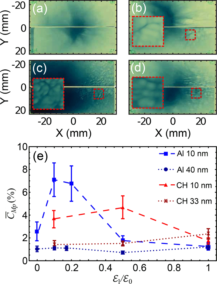
Figure 2. Example proton spatial-intensity profile at 2.2 MeV for (a)
 ${\mathcal{E}}_{1}={\mathcal{E}}_{0}$
, (b)
${\mathcal{E}}_{1}={\mathcal{E}}_{0}$
, (b)
 ${\mathcal{E}}_{1}=0.01{\mathcal{E}}_{0}$
, (c)
${\mathcal{E}}_{1}=0.01{\mathcal{E}}_{0}$
, (c)
 ${\mathcal{E}}_{1}=0.1{\mathcal{E}}_{0}$
and (d)
${\mathcal{E}}_{1}=0.1{\mathcal{E}}_{0}$
and (d)
 ${\mathcal{E}}_{1}=0.2{\mathcal{E}}_{0}$
for an
${\mathcal{E}}_{1}=0.2{\mathcal{E}}_{0}$
for an
 $l=10~\text{nm}$
Al target. The dashed insets show a magnified region, highlighting the filamentary structures. (e) Degree of structure
$l=10~\text{nm}$
Al target. The dashed insets show a magnified region, highlighting the filamentary structures. (e) Degree of structure
 $\overline{C}_{Mp}$
present in the proton beam at 2.2 MeV as a function of
$\overline{C}_{Mp}$
present in the proton beam at 2.2 MeV as a function of
 ${\mathcal{E}}_{1}$
for stated foil thicknesses and materials.
${\mathcal{E}}_{1}$
for stated foil thicknesses and materials.
In order to measure the two-dimensional spatial-intensity distribution of the beam of accelerated protons, a stack of dosimetry film (radiochromic film, RCF) was positioned 50 mm from the rear side of the target. This stack had transverse dimensions of
 $50~\text{mm}\times 65~\text{mm}$
with a split along the horizontal central axis to enable additional line-of-sight diagnostics to be operated in parallel. The proton energy detection range was from 2.2 to 85 MeV. Example proton spatial-intensity profiles are shown in Figures 2(a)–2(d) for the lowest energy (2.2 MeV) protons detected from an
$50~\text{mm}\times 65~\text{mm}$
with a split along the horizontal central axis to enable additional line-of-sight diagnostics to be operated in parallel. The proton energy detection range was from 2.2 to 85 MeV. Example proton spatial-intensity profiles are shown in Figures 2(a)–2(d) for the lowest energy (2.2 MeV) protons detected from an
 $l=10~\text{nm}$
aluminium foil, as a function of
$l=10~\text{nm}$
aluminium foil, as a function of
 ${\mathcal{E}}_{1}$
. In all cases, the majority of the protons are located at a position in between the target normal and laser axes, which is consistent with previous measurements of proton acceleration in ultrathin foils undergoing RSIT[Reference Powell, King, Gray, MacLellan, Gonzalez-Izquierdo, Stockhausen, Hicks, Dover, Rusby, Carroll, Padda, Torres, Kar, Clarke, Musgrave, Najmudin, Borghesi, Neely and McKenna27, Reference King, Gray, Powell, MacLellan, Gonzalez-Izquierdo, Stockhausen, Hicks, Dover, Rusby, Carroll, Padda, Torres, Kar, Clarke, Musgrave, Najmudin, Borghesi, Neely and McKenna35]. However, when the temporal intensity profile is modified with the addition of a significant second pulse (
${\mathcal{E}}_{1}$
. In all cases, the majority of the protons are located at a position in between the target normal and laser axes, which is consistent with previous measurements of proton acceleration in ultrathin foils undergoing RSIT[Reference Powell, King, Gray, MacLellan, Gonzalez-Izquierdo, Stockhausen, Hicks, Dover, Rusby, Carroll, Padda, Torres, Kar, Clarke, Musgrave, Najmudin, Borghesi, Neely and McKenna27, Reference King, Gray, Powell, MacLellan, Gonzalez-Izquierdo, Stockhausen, Hicks, Dover, Rusby, Carroll, Padda, Torres, Kar, Clarke, Musgrave, Najmudin, Borghesi, Neely and McKenna35]. However, when the temporal intensity profile is modified with the addition of a significant second pulse (
 ${\mathcal{E}}_{2}>0.5{\mathcal{E}}_{0}$
), filamentary structures begin to appear in the lower energy component of the proton beam. These structures are predominately located in the laser axis direction. This second pulse may provide the protons with additional energy due to hybrid processes during RSIT[Reference Higginson, Gray, King, Dance, Williamson, Butler, Wilson, Capdessus, Armstrong, Green, Hawkes, Martin, Wei, Mirfayzi, Yuan, Kar, Borghesi, Clarke, Neely and McKenna23], which may enable the proton structures to be observed on the RCF.
${\mathcal{E}}_{2}>0.5{\mathcal{E}}_{0}$
), filamentary structures begin to appear in the lower energy component of the proton beam. These structures are predominately located in the laser axis direction. This second pulse may provide the protons with additional energy due to hybrid processes during RSIT[Reference Higginson, Gray, King, Dance, Williamson, Butler, Wilson, Capdessus, Armstrong, Green, Hawkes, Martin, Wei, Mirfayzi, Yuan, Kar, Borghesi, Clarke, Neely and McKenna23], which may enable the proton structures to be observed on the RCF.
The structures in the proton beam are only observed at low energies. Similar patterns observed in surface damage to a filter at the front of the stack of dosimetry (RCF) film indicate that even lower energy protons or heavier ions may exhibit similar filamentation. However, as the ion species responsible cannot be distinguished, these observations are not considered further.
In order to quantify the degree of structure in the proton beam, we calculate the coefficient of variation,
 $C_{Mp}$
, as utilized in Refs. [Reference Scott, Brenner, Bagnoud, Clarke, Gonzalez-Izquierdo, Green, Heathcote, Powell, Rusby, Zielbauer, McKenna and Neely32, Reference MacLellan, Carroll, Gray, Booth, Gonzalez-Izquierdo, Powell, Scott, Neely and McKenna36]. This is the ratio of the spatially averaged standard deviation of the proton dose to the mean dose, expressed as a percentage. Within the region of interest, this is quasi-constant and can therefore be averaged giving a measure of structural modulation
$C_{Mp}$
, as utilized in Refs. [Reference Scott, Brenner, Bagnoud, Clarke, Gonzalez-Izquierdo, Green, Heathcote, Powell, Rusby, Zielbauer, McKenna and Neely32, Reference MacLellan, Carroll, Gray, Booth, Gonzalez-Izquierdo, Powell, Scott, Neely and McKenna36]. This is the ratio of the spatially averaged standard deviation of the proton dose to the mean dose, expressed as a percentage. Within the region of interest, this is quasi-constant and can therefore be averaged giving a measure of structural modulation
 $\overline{C}_{Mp}$
. This is achieved by sampling multiple
$\overline{C}_{Mp}$
. This is achieved by sampling multiple
 $20~\text{pixel}\times 20~\text{pixel}$
blocks within a region of
$20~\text{pixel}\times 20~\text{pixel}$
blocks within a region of
 $10~\text{mm}\times 20~\text{mm}$
, centred on the laser axis located at
$10~\text{mm}\times 20~\text{mm}$
, centred on the laser axis located at
 $X=20~\text{mm}$
and
$X=20~\text{mm}$
and
 $Y=0~\text{mm}$
. The degree of structure is shown in Figure 2(e) for a range of
$Y=0~\text{mm}$
. The degree of structure is shown in Figure 2(e) for a range of
 ${\mathcal{E}}_{1}$
,
${\mathcal{E}}_{1}$
,
 $l$
and target material. For an
$l$
and target material. For an
 $l=10~\text{nm}$
Al target,
$l=10~\text{nm}$
Al target,
 $\overline{C}_{Mp}$
increases with increasing
$\overline{C}_{Mp}$
increases with increasing
 ${\mathcal{E}}_{1}$
, peaking at
${\mathcal{E}}_{1}$
, peaking at
 ${\mathcal{E}}_{1}=0.1{\mathcal{E}}_{0}$
. As the intensity of the first pulse is further increased, the degree of structure reduces until there is no longer any significant structure present. Filamentary structures are also seen for an
${\mathcal{E}}_{1}=0.1{\mathcal{E}}_{0}$
. As the intensity of the first pulse is further increased, the degree of structure reduces until there is no longer any significant structure present. Filamentary structures are also seen for an
 $l=10~\text{nm}$
CH target indicating that similar behaviour is also present even when the target material is varied. However, for the CH target,
$l=10~\text{nm}$
CH target indicating that similar behaviour is also present even when the target material is varied. However, for the CH target,
 $\overline{C}_{Mp}$
is reduced and observed to occur for a higher value of
$\overline{C}_{Mp}$
is reduced and observed to occur for a higher value of
 ${\mathcal{E}}_{1}$
compared to the Al target. This is potentially attributed to the reduction in electron density of the CH targets (
${\mathcal{E}}_{1}$
compared to the Al target. This is potentially attributed to the reduction in electron density of the CH targets (
 $n_{eAl}=630n_{\text{crit}}$
and
$n_{eAl}=630n_{\text{crit}}$
and
 $n_{eCH}=420n_{\text{crit}}$
where
$n_{eCH}=420n_{\text{crit}}$
where
 $n_{\text{crit}}=1\times 10^{27}~\text{m}^{-3}$
for the laser wavelength of
$n_{\text{crit}}=1\times 10^{27}~\text{m}^{-3}$
for the laser wavelength of
 $1.054~\unicode[STIX]{x03BC}\text{m}$
and
$1.054~\unicode[STIX]{x03BC}\text{m}$
and
 $\unicode[STIX]{x1D6FE}\sim 1$
). For thicker targets, the degree of structure is significantly lower and there is no clear trend with
$\unicode[STIX]{x1D6FE}\sim 1$
). For thicker targets, the degree of structure is significantly lower and there is no clear trend with
 ${\mathcal{E}}_{1}$
.
${\mathcal{E}}_{1}$
.
3 Numerical modelling
To investigate the initial seeding of this behaviour, 2D PIC simulations were conducted with the fully relativistic code EPOCH[Reference Arber, Bennett, Brady, Lawrence-Douglas, Ramsay, Sircombe, Gillies, Evans, Schmitz, Bell and Ridgers37]. The simulation box was defined as a 10,000
 $\times$
11,250 grid with a spatial extent of
$\times$
11,250 grid with a spatial extent of
 $10~\unicode[STIX]{x03BC}\text{m}\times 23~\unicode[STIX]{x03BC}\text{m}$
. A singular larger simulation was also defined with a 20,000
$10~\unicode[STIX]{x03BC}\text{m}\times 23~\unicode[STIX]{x03BC}\text{m}$
. A singular larger simulation was also defined with a 20,000
 $\times$
11,250 grid and spatial extent of
$\times$
11,250 grid and spatial extent of
 $20~\unicode[STIX]{x03BC}\text{m}\times 23~\unicode[STIX]{x03BC}\text{m}$
to investigate RSIT effects. The spatial resolution in the
$20~\unicode[STIX]{x03BC}\text{m}\times 23~\unicode[STIX]{x03BC}\text{m}$
to investigate RSIT effects. The spatial resolution in the
 $z$
-direction is a factor of two higher than in the
$z$
-direction is a factor of two higher than in the
 $x$
-direction in order to provide sufficient resolution to resolve the skin depth (
$x$
-direction in order to provide sufficient resolution to resolve the skin depth (
 $l_{s}=c/\unicode[STIX]{x1D714}_{pe}$
, where
$l_{s}=c/\unicode[STIX]{x1D714}_{pe}$
, where
 $\unicode[STIX]{x1D714}_{pe}$
is the plasma frequency)[Reference Rozmus and Tikhonchuk38] without significantly increasing computational requirements. The plasma was defined as an
$\unicode[STIX]{x1D714}_{pe}$
is the plasma frequency)[Reference Rozmus and Tikhonchuk38] without significantly increasing computational requirements. The plasma was defined as an
 $\text{Al}^{11+}$
slab with a thickness of 10 nm and a density of
$\text{Al}^{11+}$
slab with a thickness of 10 nm and a density of
 $60n_{\text{crit}}$
with 2-nm-thick proton contamination layers with a density of
$60n_{\text{crit}}$
with 2-nm-thick proton contamination layers with a density of
 $60n_{\text{crit}}$
at the front and rear of the target. These contamination layers have been approximated to the hydrogen density within ethanol (a common hydrocarbon found in laboratories) and the thickness is assumed to be 2 nm. To simplify the analysis, carbon and oxygen ions are not included, but this is acceptable because the proton layer expands faster due to the higher charge-to-mass ratio of protons. The ions are neutralized with a corresponding electron population, with a peak density of
$60n_{\text{crit}}$
at the front and rear of the target. These contamination layers have been approximated to the hydrogen density within ethanol (a common hydrocarbon found in laboratories) and the thickness is assumed to be 2 nm. To simplify the analysis, carbon and oxygen ions are not included, but this is acceptable because the proton layer expands faster due to the higher charge-to-mass ratio of protons. The ions are neutralized with a corresponding electron population, with a peak density of
 $660n_{\text{crit}}$
, and the initial electron and ion temperatures set at 10 eV. The number of particles per cell was initially 350 per species. The incoming laser was linearly polarized along the
$660n_{\text{crit}}$
, and the initial electron and ion temperatures set at 10 eV. The number of particles per cell was initially 350 per species. The incoming laser was linearly polarized along the
 $x$
-axis, propagating along the
$x$
-axis, propagating along the
 $z$
-axis and focused at
$z$
-axis and focused at
 $Z=0$
at the front of the target to an FWHM diameter of
$Z=0$
at the front of the target to an FWHM diameter of
 $5~\unicode[STIX]{x03BC}\text{m}$
, with a pulse duration of
$5~\unicode[STIX]{x03BC}\text{m}$
, with a pulse duration of
 $\unicode[STIX]{x1D70F}_{L}=400~\text{fs}$
FWHM. The spot size and pulse duration have been reduced to decrease the computational requirements of the system. While this may subtly affect the formation of the structures, this will still enable the overall trend in the amount of proton structure to be investigated for varying energies in the first pulse.
$\unicode[STIX]{x1D70F}_{L}=400~\text{fs}$
FWHM. The spot size and pulse duration have been reduced to decrease the computational requirements of the system. While this may subtly affect the formation of the structures, this will still enable the overall trend in the amount of proton structure to be investigated for varying energies in the first pulse.
The simulations are designed to investigate, with high spatial resolution, the seeding of the proton beam structures at early times in the interaction. As such the overall simulation time was 0.5 ps with a time step of
 $2.8\times 10^{-18}~\text{s}$
. An additional simulation was run for 0.7 ps to investigate the effects of RSIT. The energy in this pulse was varied from
$2.8\times 10^{-18}~\text{s}$
. An additional simulation was run for 0.7 ps to investigate the effects of RSIT. The energy in this pulse was varied from
 ${\mathcal{E}}_{1}=0.01{\mathcal{E}}_{0}$
to
${\mathcal{E}}_{1}=0.01{\mathcal{E}}_{0}$
to
 ${\mathcal{E}}_{1}=1.0{\mathcal{E}}_{0}$
where
${\mathcal{E}}_{1}=1.0{\mathcal{E}}_{0}$
where
 ${\mathcal{E}}_{0}=I_{0}\unicode[STIX]{x1D70F}_{L}$
and
${\mathcal{E}}_{0}=I_{0}\unicode[STIX]{x1D70F}_{L}$
and
 $I_{0}=2\times 10^{20}~\text{W}\cdot \text{cm}^{-2}$
. The time
$I_{0}=2\times 10^{20}~\text{W}\cdot \text{cm}^{-2}$
. The time
 $t=0$
is defined as when the peak of the first pulse reaches the front of the target. A second pulse was defined with the same duration and diameter, separated from the first pulse by 1 ps with
$t=0$
is defined as when the peak of the first pulse reaches the front of the target. A second pulse was defined with the same duration and diameter, separated from the first pulse by 1 ps with
 ${\mathcal{E}}_{2}={\mathcal{E}}_{0}-{\mathcal{E}}_{1}$
.
${\mathcal{E}}_{2}={\mathcal{E}}_{0}-{\mathcal{E}}_{1}$
.
When the interaction begins, electrons are heated and injected into the target due to vacuum heating and/or resonance absorption. As the intensity increases, additional fast electrons are produced and injected into the target at a frequency of
 $2\unicode[STIX]{x1D714}_{L}$
due to
$2\unicode[STIX]{x1D714}_{L}$
due to
 $\mathbf{j}\times \mathbf{B}$
heating[Reference Wilks39]. In order for the fast electrons to propagate through the target, a return current is drawn to satisfy charge neutrality requirements[Reference Bell, Davies, Guerin and Ruhl40]. This results in counter-streaming electron populations that lead to the growth of the Weibel instability, resulting in the formation of azimuthal magnetic field perturbations[Reference Weibel29]. For thicker, solid density targets, collisions will act to suppress the growth of the Weibel instability[Reference Wallace, Brackbill, Cranfill, Forslund and Mason41]. The growth rate of the Weibel instability between a fast electron current stream and neutralizing return current can be approximated as
$\mathbf{j}\times \mathbf{B}$
heating[Reference Wilks39]. In order for the fast electrons to propagate through the target, a return current is drawn to satisfy charge neutrality requirements[Reference Bell, Davies, Guerin and Ruhl40]. This results in counter-streaming electron populations that lead to the growth of the Weibel instability, resulting in the formation of azimuthal magnetic field perturbations[Reference Weibel29]. For thicker, solid density targets, collisions will act to suppress the growth of the Weibel instability[Reference Wallace, Brackbill, Cranfill, Forslund and Mason41]. The growth rate of the Weibel instability between a fast electron current stream and neutralizing return current can be approximated as
 $\unicode[STIX]{x1D6E4}_{W}\approx \sqrt{n_{f}/n_{r}}\unicode[STIX]{x1D714}_{L}/\sqrt{\unicode[STIX]{x1D6FE}_{r}}$
, where
$\unicode[STIX]{x1D6E4}_{W}\approx \sqrt{n_{f}/n_{r}}\unicode[STIX]{x1D714}_{L}/\sqrt{\unicode[STIX]{x1D6FE}_{r}}$
, where
 $n_{f}$
is the fast electron density, and
$n_{f}$
is the fast electron density, and
 $n_{r}$
and
$n_{r}$
and
 $\unicode[STIX]{x1D6FE}_{r}$
are the return current density and Lorentz factor, respectively[Reference Göde, Rödel, Zeil, Mishra, Gauthier, Brack, Kluge, MacDonald, Metzkes, Obst, Rehwald, Ruyer, Schlenvoigt, Schumaker, Sommer, Cowan, Schramm, Glenzer and Fiuza33]. As the intensity of the laser pulse exceeds
$\unicode[STIX]{x1D6FE}_{r}$
are the return current density and Lorentz factor, respectively[Reference Göde, Rödel, Zeil, Mishra, Gauthier, Brack, Kluge, MacDonald, Metzkes, Obst, Rehwald, Ruyer, Schlenvoigt, Schumaker, Sommer, Cowan, Schramm, Glenzer and Fiuza33]. As the intensity of the laser pulse exceeds
 $a_{0}=1$
,
$a_{0}=1$
,
 $n_{f}\rightarrow n_{\text{crit}}$
due to the optimization of the
$n_{f}\rightarrow n_{\text{crit}}$
due to the optimization of the
 $\mathbf{j}\times \mathbf{B}$
heating. As the return current must be able to balance the fast electron current,
$\mathbf{j}\times \mathbf{B}$
heating. As the return current must be able to balance the fast electron current,
 $n_{r}>n_{f}$
, therefore, within the target, the growth rate is maximized close to the critical surface where
$n_{r}>n_{f}$
, therefore, within the target, the growth rate is maximized close to the critical surface where
 $n_{r}\sim n_{\text{crit}}$
and as the intensity approaches
$n_{r}\sim n_{\text{crit}}$
and as the intensity approaches
 $a_{0}=1$
. Note, the instability continues to grow even when this condition is not met, albeit more slowly, and as the target expands,
$a_{0}=1$
. Note, the instability continues to grow even when this condition is not met, albeit more slowly, and as the target expands,
 $n_{r}$
also reduces throughout the volume, due to the overall reduction in peak density, allowing faster growth. The formation of strong electrostatic sheath fields at the front and rear surfaces also acts to reflect both the slower moving electrons and a significant percentage of the fast electron population back into the target. This results in a continual, recirculating population[Reference Sentoku, Cowan, Kemp and Ruhl42] that will facilitate constant streaming behaviour, allowing the Weibel instability to grow until it reaches saturation, producing strong quasi-static azimuthal magnetic filaments that extend across the longitudinal extent of the target.
$n_{r}$
also reduces throughout the volume, due to the overall reduction in peak density, allowing faster growth. The formation of strong electrostatic sheath fields at the front and rear surfaces also acts to reflect both the slower moving electrons and a significant percentage of the fast electron population back into the target. This results in a continual, recirculating population[Reference Sentoku, Cowan, Kemp and Ruhl42] that will facilitate constant streaming behaviour, allowing the Weibel instability to grow until it reaches saturation, producing strong quasi-static azimuthal magnetic filaments that extend across the longitudinal extent of the target.

Figure 3. 2D simulation results at
 $t=-0.325~\text{ps}$
(where
$t=-0.325~\text{ps}$
(where
 $t=0$
is the time when the peak of the first pulse reaches the target) for a laser pulse with
$t=0$
is the time when the peak of the first pulse reaches the target) for a laser pulse with
 ${\mathcal{E}}_{1}=0.1{\mathcal{E}}_{0}$
showing the spatial profile of (a) the transverse magnetic field,
${\mathcal{E}}_{1}=0.1{\mathcal{E}}_{0}$
showing the spatial profile of (a) the transverse magnetic field,
 $B_{Y}$
and (b) the electron density,
$B_{Y}$
and (b) the electron density,
 $n_{e}$
. In all cases, the laser enters the simulation box from the left along the
$n_{e}$
. In all cases, the laser enters the simulation box from the left along the
 $x=0$
axis.
$x=0$
axis.
At the same time, these large electrostatic sheath fields formed at the front and rear of the target also result in the acceleration of ions via sheath acceleration[Reference Wilks, Langdon, Cowan, Roth, Singh, Hatchett, Key, Pennington, MacKinnon and Snavely8]. Protons sourced from the target and surface contamination layers are accelerated first due to their higher charge-to-mass ratio. This results in an accelerated layer of protons that propagates in front of the
 $\text{Al}^{11+}$
ions[Reference Dover, Palmer, Streeter, Ahmed, Albertazzi, Borghesi, Carroll, Fuchs, Heathcote, Hilz, Kakolee, Kar, Kodama, Kon, MacLellan, McKenna, Nagel, Neely, Notley, Nakatsutsumi, Prasad, Scott, Tampo, Zepf, Schreiber and Najmudin43].
$\text{Al}^{11+}$
ions[Reference Dover, Palmer, Streeter, Ahmed, Albertazzi, Borghesi, Carroll, Fuchs, Heathcote, Hilz, Kakolee, Kar, Kodama, Kon, MacLellan, McKenna, Nagel, Neely, Notley, Nakatsutsumi, Prasad, Scott, Tampo, Zepf, Schreiber and Najmudin43].
Figure 3(a) shows the behaviour of the transverse magnetic field,
 $B_{Y}$
, in the system at
$B_{Y}$
, in the system at
 $t=-0.325~\text{ps}$
for
$t=-0.325~\text{ps}$
for
 ${\mathcal{E}}_{1}=0.1{\mathcal{E}}_{0}$
. Large-scale azimuthal fields are formed at the front and rear critical surfaces of the target, as expected from typical intense laser–solid interactions[Reference Sarri, Macchi, Cecchetti, Kar, Liseykina, Yang, Dieckmann, Fuchs, Galimberti, Gizzi, Jung, Kourakis, Osterholz, Pegoraro, Robinson, Romagnani, Willi and Borghesi44]. However, within the region of the focal spot of the laser, periodic magnetic field structures in the
${\mathcal{E}}_{1}=0.1{\mathcal{E}}_{0}$
. Large-scale azimuthal fields are formed at the front and rear critical surfaces of the target, as expected from typical intense laser–solid interactions[Reference Sarri, Macchi, Cecchetti, Kar, Liseykina, Yang, Dieckmann, Fuchs, Galimberti, Gizzi, Jung, Kourakis, Osterholz, Pegoraro, Robinson, Romagnani, Willi and Borghesi44]. However, within the region of the focal spot of the laser, periodic magnetic field structures in the
 $x$
-direction have formed across the longitudinal extent of the target due to the Weibel instability. This can act to distort the large-scale rear surface fields. These structures begin small in spatial extent, growing larger as the instability saturates. Initially, these are on the order of kilotesla and have the effect of driving similar periodic structures in the expanding electron population as shown in Figure 3(b). Likewise, due to space-charge separation, the now bunched electron population draws the accelerating protons into the same periodic structure. This is predominately seen at the rear of the expanding proton layer, which corresponds to the lowest energy protons.
$x$
-direction have formed across the longitudinal extent of the target due to the Weibel instability. This can act to distort the large-scale rear surface fields. These structures begin small in spatial extent, growing larger as the instability saturates. Initially, these are on the order of kilotesla and have the effect of driving similar periodic structures in the expanding electron population as shown in Figure 3(b). Likewise, due to space-charge separation, the now bunched electron population draws the accelerating protons into the same periodic structure. This is predominately seen at the rear of the expanding proton layer, which corresponds to the lowest energy protons.
The final proton structures are shown in Figure 4 for
 ${\mathcal{E}}_{1}=0.01{\mathcal{E}}_{0}$
and
${\mathcal{E}}_{1}=0.01{\mathcal{E}}_{0}$
and
 ${\mathcal{E}}_{1}=0.1{\mathcal{E}}_{0}$
at
${\mathcal{E}}_{1}=0.1{\mathcal{E}}_{0}$
at
 $t=0~\text{ps}$
and
$t=0~\text{ps}$
and
 $t=-0.2~\text{ps}$
, respectively, just prior to the proton population leaving the simulation box in each case. As can be seen, the protons exhibit transverse filamentary structures imprinted from the structured electron population early in the interaction. The
$t=-0.2~\text{ps}$
, respectively, just prior to the proton population leaving the simulation box in each case. As can be seen, the protons exhibit transverse filamentary structures imprinted from the structured electron population early in the interaction. The
 ${\mathcal{E}}_{1}=0.01{\mathcal{E}}_{0}$
case exhibits a lower frequency of filaments compared with the
${\mathcal{E}}_{1}=0.01{\mathcal{E}}_{0}$
case exhibits a lower frequency of filaments compared with the
 ${\mathcal{E}}_{1}=0.1{\mathcal{E}}_{0}$
case. This is due to the extent of expansion of the proton layer prior to the formation of the magnetic field structures associated with the Weibel instability, which will be explored later.
${\mathcal{E}}_{1}=0.1{\mathcal{E}}_{0}$
case. This is due to the extent of expansion of the proton layer prior to the formation of the magnetic field structures associated with the Weibel instability, which will be explored later.
Figure 4(c) illustrates the temporal behaviour of the filaments for the
 ${\mathcal{E}}_{1}=0.1{\mathcal{E}}_{0}$
case. To fully show this behaviour a larger simulation was conducted as previously defined in order to prevent the protons from leaving the simulation box. The filaments maintain their structure from
${\mathcal{E}}_{1}=0.1{\mathcal{E}}_{0}$
case. To fully show this behaviour a larger simulation was conducted as previously defined in order to prevent the protons from leaving the simulation box. The filaments maintain their structure from
 $t=-0.4~\text{ps}$
to
$t=-0.4~\text{ps}$
to
 $t=-0.15~\text{ps}$
. At
$t=-0.15~\text{ps}$
. At
 $t=-0.15~\text{ps}$
, the target becomes relativistically transparent to the laser pulse. As the remainder of the laser light propagates through the target, electrons are directly accelerated resulting in dense bunches that travel through the expanding proton layer[Reference Gonzalez-Izquierdo, Gray, King, Dance, Wilson, McCreadie, Butler, Capdessus, Hawkes, Green, Borghesi, Neely and McKenna20, Reference Powell, King, Gray, MacLellan, Gonzalez-Izquierdo, Stockhausen, Hicks, Dover, Rusby, Carroll, Padda, Torres, Kar, Clarke, Musgrave, Najmudin, Borghesi, Neely and McKenna27]. Although this can modify the detail of the structures formed in the proton beam, we find that the structure is still present after transparency. The sizes of the structures in the proton beam will be modified over the large propagation distance that the diverging beam of protons travels in the experiment, which prevents a quantitative comparison with the size of the structures in the simulation. Nevertheless, understanding the initial seeding of the proton filaments on the rising edge of the first pulse provides a good approximation of the final degree of structure present in the beam, as will be shown below.
$t=-0.15~\text{ps}$
, the target becomes relativistically transparent to the laser pulse. As the remainder of the laser light propagates through the target, electrons are directly accelerated resulting in dense bunches that travel through the expanding proton layer[Reference Gonzalez-Izquierdo, Gray, King, Dance, Wilson, McCreadie, Butler, Capdessus, Hawkes, Green, Borghesi, Neely and McKenna20, Reference Powell, King, Gray, MacLellan, Gonzalez-Izquierdo, Stockhausen, Hicks, Dover, Rusby, Carroll, Padda, Torres, Kar, Clarke, Musgrave, Najmudin, Borghesi, Neely and McKenna27]. Although this can modify the detail of the structures formed in the proton beam, we find that the structure is still present after transparency. The sizes of the structures in the proton beam will be modified over the large propagation distance that the diverging beam of protons travels in the experiment, which prevents a quantitative comparison with the size of the structures in the simulation. Nevertheless, understanding the initial seeding of the proton filaments on the rising edge of the first pulse provides a good approximation of the final degree of structure present in the beam, as will be shown below.
It should be noted that the streaming of the fast electrons with the return current and the Weibel growth also occurs in thicker targets. However, reduced scale simulations incorporating collisional effects indicate that the electron collisions with
 $\text{Al}^{11+}$
ions act to damp out the growth of these magnetic field perturbations, resulting in a smooth proton beam. As the target thickness is increased, the streaming electrons are able to collide more readily with the background ion population, preventing significant instability growth[Reference Kemp, Sentoku, Sotnikov and Wilks45]. Therefore, this effect will only be seen for targets below a certain thickness, which is consistent with the experimental measurements shown in Figure 2(e).
$\text{Al}^{11+}$
ions act to damp out the growth of these magnetic field perturbations, resulting in a smooth proton beam. As the target thickness is increased, the streaming electrons are able to collide more readily with the background ion population, preventing significant instability growth[Reference Kemp, Sentoku, Sotnikov and Wilks45]. Therefore, this effect will only be seen for targets below a certain thickness, which is consistent with the experimental measurements shown in Figure 2(e).

Figure 4. 2D simulation proton density maps of the expanding rear proton layer for (a)
 ${\mathcal{E}}_{1}=0.01{\mathcal{E}}_{0}$
at
${\mathcal{E}}_{1}=0.01{\mathcal{E}}_{0}$
at
 $t=0~\text{ps}$
and (b)
$t=0~\text{ps}$
and (b)
 ${\mathcal{E}}_{1}=0.1{\mathcal{E}}_{0}$
at
${\mathcal{E}}_{1}=0.1{\mathcal{E}}_{0}$
at
 $t=-0.2~\text{ps}$
. These example times are chosen such that there is a similar degree of proton layer expansion. (c) Time–space plot of proton density for
$t=-0.2~\text{ps}$
. These example times are chosen such that there is a similar degree of proton layer expansion. (c) Time–space plot of proton density for
 ${\mathcal{E}}_{1}=0.1{\mathcal{E}}_{0}$
relative to the proton motion sampled along the transverse direction
${\mathcal{E}}_{1}=0.1{\mathcal{E}}_{0}$
relative to the proton motion sampled along the transverse direction
 $0.25~\unicode[STIX]{x03BC}\text{m}$
from the rear edge of the proton layer. The white dashed line denotes the onset of RSIT. Note the density is normalized to the average proton density at each point in time to compensate for expansion.
$0.25~\unicode[STIX]{x03BC}\text{m}$
from the rear edge of the proton layer. The white dashed line denotes the onset of RSIT. Note the density is normalized to the average proton density at each point in time to compensate for expansion.

Figure 5. Time–space plot of the transverse magnetic field in the centre of the target (
 $Z=5~\text{nm}$
) for a solid density,
$Z=5~\text{nm}$
) for a solid density,
 $l=10~\text{nm}$
Al target for (a)
$l=10~\text{nm}$
Al target for (a)
 ${\mathcal{E}}_{1}=0.01{\mathcal{E}}_{0}$
and (b)
${\mathcal{E}}_{1}=0.01{\mathcal{E}}_{0}$
and (b)
 ${\mathcal{E}}_{1}=0.1{\mathcal{E}}_{0}$
. (c) and (d) Spatial Fourier transform of the magnetic field in (a) and (b), respectively.
${\mathcal{E}}_{1}=0.1{\mathcal{E}}_{0}$
. (c) and (d) Spatial Fourier transform of the magnetic field in (a) and (b), respectively.

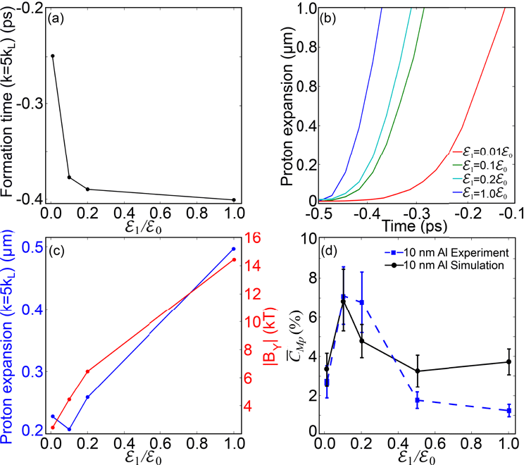
Figure 6. Plots of simulation results showing (a) formation time of the magnetic field structures as a function of
 ${\mathcal{E}}_{1}$
, (b) longitudinal position,
${\mathcal{E}}_{1}$
, (b) longitudinal position,
 $Z$
, of the back of the sheath-accelerated proton layer sampled at
$Z$
, of the back of the sheath-accelerated proton layer sampled at
 $X=0$
as a function of time, for each given
$X=0$
as a function of time, for each given
 ${\mathcal{E}}_{1}$
, (c) longitudinal position,
${\mathcal{E}}_{1}$
, (c) longitudinal position,
 $Z$
, of the rear of the expanding proton layer at
$Z$
, of the rear of the expanding proton layer at
 $X=0$
(blue) and absolute azimuthal magnetic field strength (red) at the point in time at which the magnetic field structure formation begins as a function of
$X=0$
(blue) and absolute azimuthal magnetic field strength (red) at the point in time at which the magnetic field structure formation begins as a function of
 ${\mathcal{E}}_{1}$
, and (d) comparison of simulated and experimental proton
${\mathcal{E}}_{1}$
, and (d) comparison of simulated and experimental proton
 $\overline{C}_{Mp}$
for an Al
$\overline{C}_{Mp}$
for an Al
 $l=10~\text{nm}$
target as a function of
$l=10~\text{nm}$
target as a function of
 ${\mathcal{E}}_{1}$
.
${\mathcal{E}}_{1}$
.
To aid in the understanding of the magnetic field growth, the temporal evolution of the transverse magnetic field structures at
 $Z=5~\text{nm}$
(i.e., at the centre of the target) is shown in Figure 5 for
$Z=5~\text{nm}$
(i.e., at the centre of the target) is shown in Figure 5 for
 ${\mathcal{E}}_{1}=0.01{\mathcal{E}}_{0}$
(Figure 5(a)) and
${\mathcal{E}}_{1}=0.01{\mathcal{E}}_{0}$
(Figure 5(a)) and
 ${\mathcal{E}}_{1}=0.1{\mathcal{E}}_{0}$
(Figure 5(b)). For
${\mathcal{E}}_{1}=0.1{\mathcal{E}}_{0}$
(Figure 5(b)). For
 ${\mathcal{E}}_{1}=0.1{\mathcal{E}}_{0}$
, the structures begin to form at
${\mathcal{E}}_{1}=0.1{\mathcal{E}}_{0}$
, the structures begin to form at
 $t=-0.38~\text{ps}$
, whereas for
$t=-0.38~\text{ps}$
, whereas for
 ${\mathcal{E}}_{1}=0.01{\mathcal{E}}_{0}$
the formation time is delayed to
${\mathcal{E}}_{1}=0.01{\mathcal{E}}_{0}$
the formation time is delayed to
 $t=-0.25~\text{ps}$
as it takes longer for the intensity to approach
$t=-0.25~\text{ps}$
as it takes longer for the intensity to approach
 $a_{0}\approx 1$
. The structures initially grow at large spatial wavenumbers,
$a_{0}\approx 1$
. The structures initially grow at large spatial wavenumbers,
 $k$
, before reducing down to sizes on the order of the laser wavenumber
$k$
, before reducing down to sizes on the order of the laser wavenumber
 $k_{L}$
due to saturation of the Weibel instability. Structures of a similar spatial scale are also observed to grow and evolve in the same manner in simulations reported by Thaury et al.
[Reference Thaury, Mora, Héron, Adam and Antonsen46] for comparable densities and laser parameters. The linear growth rates are found to be
$k_{L}$
due to saturation of the Weibel instability. Structures of a similar spatial scale are also observed to grow and evolve in the same manner in simulations reported by Thaury et al.
[Reference Thaury, Mora, Héron, Adam and Antonsen46] for comparable densities and laser parameters. The linear growth rates are found to be
 $\unicode[STIX]{x1D6E4}\sim 0.03\unicode[STIX]{x1D714}_{L}$
and
$\unicode[STIX]{x1D6E4}\sim 0.03\unicode[STIX]{x1D714}_{L}$
and
 $\unicode[STIX]{x1D6E4}\sim 0.05\unicode[STIX]{x1D714}_{L}$
for
$\unicode[STIX]{x1D6E4}\sim 0.05\unicode[STIX]{x1D714}_{L}$
for
 ${\mathcal{E}}_{1}=0.01{\mathcal{E}}_{0}$
and
${\mathcal{E}}_{1}=0.01{\mathcal{E}}_{0}$
and
 ${\mathcal{E}}_{1}=0.1{\mathcal{E}}_{0}$
, respectively, where
${\mathcal{E}}_{1}=0.1{\mathcal{E}}_{0}$
, respectively, where
 $\unicode[STIX]{x1D714}_{L}$
is the angular laser frequency. This is also comparable to the theory reported by Thaury et al.
[Reference Thaury, Mora, Héron, Adam and Antonsen46], for which a growth rate of
$\unicode[STIX]{x1D714}_{L}$
is the angular laser frequency. This is also comparable to the theory reported by Thaury et al.
[Reference Thaury, Mora, Héron, Adam and Antonsen46], for which a growth rate of
 $\unicode[STIX]{x1D6E4}\sim 0.029\unicode[STIX]{x1D714}_{L}$
is determined for comparable laser–plasma conditions. Once the large-scale structures are established, they appear fixed in space throughout the simulation until RSIT occurs and the laser begins to propagate through the target. This results in the magnetic field structures dissipating, but the now structured proton beam receives a small increase in energy due to transparency enhancement[Reference Powell, King, Gray, MacLellan, Gonzalez-Izquierdo, Stockhausen, Hicks, Dover, Rusby, Carroll, Padda, Torres, Kar, Clarke, Musgrave, Najmudin, Borghesi, Neely and McKenna27]. This may provide the lower energy protons (that contain an observable degree of filamentary structure) with sufficient energy to exceed the lower detection threshold (
$\unicode[STIX]{x1D6E4}\sim 0.029\unicode[STIX]{x1D714}_{L}$
is determined for comparable laser–plasma conditions. Once the large-scale structures are established, they appear fixed in space throughout the simulation until RSIT occurs and the laser begins to propagate through the target. This results in the magnetic field structures dissipating, but the now structured proton beam receives a small increase in energy due to transparency enhancement[Reference Powell, King, Gray, MacLellan, Gonzalez-Izquierdo, Stockhausen, Hicks, Dover, Rusby, Carroll, Padda, Torres, Kar, Clarke, Musgrave, Najmudin, Borghesi, Neely and McKenna27]. This may provide the lower energy protons (that contain an observable degree of filamentary structure) with sufficient energy to exceed the lower detection threshold (
 ${\sim}2.2~\text{MeV}$
) of the RCF, enabling them to be detected experimentally.
${\sim}2.2~\text{MeV}$
) of the RCF, enabling them to be detected experimentally.
For the magnetic field structures, and thus the electron structures, to influence the beam of accelerated protons, they have to form early enough in the interaction before the proton layer has significantly expanded from the bulk of the target. As the intensity of the first pulse is increased, the proton layer will expand to such an extent that it will be outside the influence of the magnetic field structures prior to their formation. As the intensity of the first pulse is lowered, both the formation time of the magnetic field structures and the degree of proton layer expansion are reduced at differing rates. This leads to a parameter space for which the degree of structure in the proton beam is maximized for the least amount of initial proton layer expansion and fastest azimuthal magnetic field formation.
Figure 6(a) shows the formation time of the magnetic structures, defined as the time at which the structure appears at
 $k=5k_{L}$
. For comparison, Figure 6(b) shows the degree of proton layer expansion, defined as the longitudinal position,
$k=5k_{L}$
. For comparison, Figure 6(b) shows the degree of proton layer expansion, defined as the longitudinal position,
 $Z$
, of the rear of the expanding proton layer at
$Z$
, of the rear of the expanding proton layer at
 $X=0$
, as a function of time for various values of
$X=0$
, as a function of time for various values of
 ${\mathcal{E}}_{1}$
. These two plots enable the extent of proton layer expansion at the formation time of the magnetic field structures to be plotted as a function of
${\mathcal{E}}_{1}$
. These two plots enable the extent of proton layer expansion at the formation time of the magnetic field structures to be plotted as a function of
 ${\mathcal{E}}_{1}$
, as shown in Figure 6(c). As can be seen, a minimum occurs for
${\mathcal{E}}_{1}$
, as shown in Figure 6(c). As can be seen, a minimum occurs for
 ${\mathcal{E}}_{1}=0.1{\mathcal{E}}_{0}$
. Also plotted is the magnitude of the maximum field strength of the magnetic field structures at formation time. This tends to increase with
${\mathcal{E}}_{1}=0.1{\mathcal{E}}_{0}$
. Also plotted is the magnitude of the maximum field strength of the magnetic field structures at formation time. This tends to increase with
 ${\mathcal{E}}_{1}$
.
${\mathcal{E}}_{1}$
.
Figure 6(d) shows a comparison between the degree of structure within the proton beam from the simulation and the experiment. Good agreement is found in the trend for the
 $l=10~\text{nm}$
Al target and when compared with the simulation data shown in Figure 6(c), an inverse correlation to the degree of proton layer expansion at the time of magnetic field structure formation can also be seen. The simulations tend to over-predict the amount of structure present in the
$l=10~\text{nm}$
Al target and when compared with the simulation data shown in Figure 6(c), an inverse correlation to the degree of proton layer expansion at the time of magnetic field structure formation can also be seen. The simulations tend to over-predict the amount of structure present in the
 ${\mathcal{E}}_{1}=0.5{\mathcal{E}}_{0}$
and
${\mathcal{E}}_{1}=0.5{\mathcal{E}}_{0}$
and
 ${\mathcal{E}}_{1}={\mathcal{E}}_{0}$
cases. This may be due to the smaller pulse duration and focal spot size compared with the experiment (due to computational constraints). The pulse duration can affect both the expansion time and growth rate of the Weibel instability in a nonlinear fashion.
${\mathcal{E}}_{1}={\mathcal{E}}_{0}$
cases. This may be due to the smaller pulse duration and focal spot size compared with the experiment (due to computational constraints). The pulse duration can affect both the expansion time and growth rate of the Weibel instability in a nonlinear fashion.
4 Summary
Experimental and simulation studies of nanometre-thick foil interactions with intense laser pulses have suggested radiation pressure perturbations at the front surface give rise to unstable behaviour due to a Rayleigh–Taylor-like instability[Reference Sgattoni, Sinigardi, Fedeli, Pegoraro and Macchi25, Reference Palmer, Schreiber, Nagel, Dover, Bellei, Beg, Bott, Clarke, Dangor, Hassan, Hilz, Jung, Kneip, Mangles, Lancaster, Rehman, Robinson, Spindloe, Szerypo, Tatarakis, Yeung, Zepf and Najmudin26]. This work does not preclude the explanation for interactions with high contrast and sharp rising edge intensity profiles where the radiation pressure will be dominant. Here, the formation of the proton structures can be seen at comparatively low intensities of
 ${\sim}10^{18}{-}10^{19}~\text{W}\cdot \text{cm}^{-2}$
and for relatively long pulse durations of 1 ps. The formation of the magnetic field structures in the simulations indicates almost synchronous growth across the entire longitudinal extent of the plasma bulk and Rayleigh–Taylor-like instability would typically only occur at the front surface. The presence of such an instability cannot be dismissed, but if it does grow, it would likely be masked by the growth of the Weibel instability for these laser and target parameters.
${\sim}10^{18}{-}10^{19}~\text{W}\cdot \text{cm}^{-2}$
and for relatively long pulse durations of 1 ps. The formation of the magnetic field structures in the simulations indicates almost synchronous growth across the entire longitudinal extent of the plasma bulk and Rayleigh–Taylor-like instability would typically only occur at the front surface. The presence of such an instability cannot be dismissed, but if it does grow, it would likely be masked by the growth of the Weibel instability for these laser and target parameters.
As such, this work demonstrates for the first time that filamentary structures detected in laser-accelerated proton beams from nanometre-thick foil targets can depend upon the formation of azimuthal magnetic field filaments, via the Weibel instability, and the initial degree of proton layer expansion. Through the use of two controllable laser pulses, of fixed combined energy, the degree of structure in the produced proton beam can be varied, providing useful insight into the underlying mechanisms and evolution of proton beam filamentary structures.
Acknowledgements
We acknowledge the use of the ARCHIE-WeST and ARCHER computers, with access to the latter provided via the Plasma Physics HEC Consortia (EP/L000237/1). This work is supported by EPSRC (grants EP/J003832/1, EP/R006202/1, EP/P007082/1 and EP/K022415/1), and the European Unions Horizon 2020 research and innovation program (grant agreement No. 654148 Laserlab-Europe). EPOCH was developed under EPSRC grant EP/G054940/1. Data associated with research published in this paper is accessible at http://dx.doi.org/10.15129/534fd2b5-626f-4590-b447-8b090155a8a8.


 Open access