


Impact Statement
We propose a new bladeless mixer, which has advantages such as efficient cleaning and contamination avoidance. Flow in a bladeless mixer must be driven by the motion, e.g. rotation, of a container. Since the container's steady rotation always leads to solid-body rotational flow of a fluid filling it, its mixing ability reduces sooner or later. However, we discover that a liquid–gas interface can sustain turbulence of a liquid partially filling a constantly rotating spherical container if the Reynolds number is large enough and the Froude number is small enough. This turbulence is not due to the interface's oscillations but sustained by internal shear flow. We also numerically demonstrate that different filling rates of liquid lead to qualitatively different turbulence, which has different mixing times and energy consumption rates. This implies that we can change the mixing properties depending on materials to be mixed only by changing the filling rate. Since this system is one of the simplest mixers, we expect a wide variety of applications.
1. Introduction
Mixing is one of the most important units in process engineering. Since we generally use stirring blades in a mixer, it is essential for efficient mixing to select an appreciate type of blade according to the materials to be mixed (Reference NagataNagata, 1975; Reference UhlUhl, 2012; Reference ZlokarnikZlokarnik, 2001). However, with the recommendation of low environmental impact, the use of stirring blades is sometimes undesirable because it requires much energy for cleaning. The use of stirring blades is also often avoided in biotechnology. Although mixing in a bioreactor is generally needed to promote cell growth, shear flow around blades can inhibit the growth or it is even lethal for fragile cells (Reference Cherry and PapoutsakisCherry & Papoutsakis, 1986; Reference Wu, Graham and Noui MehidiWu, Graham, & Noui Mehidi, 2006). In addition, since it is known that different mixing methods in a bioreactor can lead to differences in the cell growth process (Reference Sikavitsas, Bancroft and MikosSikavitsas, Bancroft, & Mikos, 2002), various types of mixer were proposed (Reference Stephenson and GraysonStephenson & Grayson, 2018). It is therefore worth proposing a new type of bladeless mixer, that may be used in biotechnology, for example.
There exist several kinds of bladeless mixers, in which flow is driven by a motion of the container. One of the simplest motions is a rotation. However, since a steady rotation of the container, irrespective of the container's shape, always leads to solid-body rotational flow of a fluid filling it, we cannot expect the steady mixing of the confined fluid. Therefore, to drive non-trivial flow in a rotating container, we have to temporally change the magnitude or the orientation of the angular velocity of the container. The latter method is widely utilized in the so-called gyroscopic mixers or planetary mixers (Reference Kure and SakaiKure & Sakai, 2021; Reference Massing, Cicko and ZiroliMassing, Cicko, & Ziroli, 2008). For this kind of mixer, where we change the orientation of the angular velocity (i.e. the precession), it was shown that a slow precession could drive turbulent flow (Reference Goto, Ishii, Kida and NishiokaGoto, Ishii, Kida, & Nishioka, 2007) and almost perfect mixing of a fluid filling a precessing sphere could be achieved by only approximately 10 spins of the container (Reference Goto, Shimizu and KawaharaGoto, Shimizu, & Kawahara, 2014b).
However, the spin-up of the solid-body rotational flow is a phenomenon for a fluid filling a container. It is unclear if this phenomenon occurs when the container is partially filled with a fluid. To clarify this fundamental but non-trivial issue, we conduct experiments (see the Appendix for the details) to visualize the flow in a constantly rotating spherical container, which is partially filled with water (figure 1a). Surprisingly, we observe complex patterns irrespective of the filling rates between  $0.2$ and
  $0.8$ (figure 1b–d). Since characteristic length scales of the visualized patterns by reflective flakes indicate the smallest eddy size, the results shown in figure 1(b–d) imply that the flow is turbulent. Note that this turbulence is caused by the presence of the liquid–gas interface because, without it, the flow must tend to solid-body rotational flow. Moreover, since the Froude number is sufficiently small in these experiments, the interface hardly oscillates. Therefore, the generation mechanism of the turbulence observed in figure 1(b–d) is essentially different from those driven by the oscillations of a liquid–gas interface (Reference Micheletti, Barrett, Doig, Baganz, Levy, Woodley and LyeMicheletti et al., 2006; Reference Reclari, Dreyer, Tissot, Obreschkow, Wurm and FarhatReclari et al., 2014; Reference Weheliye, Yianneskis and DucciWeheliye, Yianneskis, & Ducci, 2013).

Figure 1. (a) Schematic of a rotating sphere with a liquid–gas interface, and the definition of the coordinate system whose origin is set at the centre of the sphere. We set the angular velocity of the sphere as  $\boldsymbol {\omega }=(0,0,\omega )$ and the gravitational acceleration as
  $\boldsymbol {g}=(-g,0,0)$. We examine the velocity along the dashed vertical line in figures 2 and 5. (b,c,d) Experimental results. Turbulence of water partially filling a rotating sphere with the filling rate (b)
  $\varPsi =0.2$, (c)
  $0.5$ and (d)
  $0.8$. We visualize flow by seeding refractive flakes and using a laser sheet on the equatorial plane of the sphere. We have changed the colour map to amplify the contrast of the images. The radius of the sphere is 90 mm, and the spin angular velocity is
  $0.2{\rm \pi}$ rad s
 $^{-1}$; the Reynolds number is approximately
  $5.1\times 10^3$. See the Appendix for the details of the experiments.
Because of the difficulty of numerical, experimental and theoretical treatments of flow with a liquid–gas interface, and because of the intuition that non-trivial flows are not driven, there were only a few studies on the flow of a fluid, which partially fills a constantly rotating container. Among them, Reference Varley, Markaki and BrooksVarley, Markaki, and Brooks (2017) showed that the constant rotation about its horizontal axis of a cylindrical container with a liquid–gas interface resulted in a simple flow rotating with the container when the Reynolds number was low. The observed flow is different from the turbulence shown in figure 1(b–d) in a spherical container at a higher Reynolds number. Incidentally, Reference MeunierMeunier (2020) recently showed that unsteady flow was sustained in a cylindrical container rotating around its axis and tilted from the vertical direction. He also proposed that the system could be used as a bladeless mixer.
The present study aims at (i) clarifying the sustaining mechanism of turbulence (figure 1b–d) in a spherical container which is constantly rotating about a horizontal axis, and (ii) evaluating the mixing performance of this system towards future industrial applications as a bladeless mixer. In the present experimental apparatus, however, we can observe and measure flow only on the equatorial plane (see the Appendix). It is therefore difficult to experimentally achieve the first aim, and it is also difficult to evaluate the mixing performance in experiments. Therefore, we conduct direct numerical simulations (DNS) of liquid–gas flow in a rotating spherical container to show that (i) turbulence is sustained by vortex stretching in internal shear flow around a counter-rotating pair of container-size vortices, and (ii) almost perfect mixing is achieved after approximately 10 revolutions of the container when the filling rate is less than approximately 0.5.
2. Numerical method
2.1 Governing equations
We investigate two-phase flow of liquid and gas in a rotating spherical container. As depicted in figure 1(a), the spherical container with radius  $R$ rotates at a constant angular velocity
  $\boldsymbol {\omega }=(0,0,\omega )$ about a horizontal axis. The gravitational acceleration
  $\boldsymbol {g}$ is
  $(-g,0,0)$. The origin of the Cartesian coordinates (
 $x,y,z$) is set at the centre of the sphere.
Let  $\varOmega$ be a three-dimensional domain which consists of a spherical fluid domain
  $\varOmega _f$ and a surrounding solid domain
  $\varOmega _s$. The mass conservation equation in
  $\varOmega$ is expressed as
  $\boldsymbol {\nabla } \boldsymbol {\cdot } \boldsymbol {u} = 0$, where
  $\boldsymbol {u}=(u,v,w)$ is the velocity vector. For fluid motion, we numerically solve the two-phase Navier–Stokes equation,
 \begin{equation} \rho\left(\frac{\partial \boldsymbol{u}}{\partial t} + \boldsymbol{u} \boldsymbol{\cdot} \boldsymbol{\nabla} \boldsymbol{u}\right) = {-} \boldsymbol{\nabla} p + \boldsymbol{\nabla} \boldsymbol{\cdot} (\mu \boldsymbol{D}(\boldsymbol{u})) + \rho \boldsymbol{g} \quad \text{in } \varOmega_{f},\end{equation}
where  $\boldsymbol {D}(\boldsymbol {u})=\boldsymbol {\nabla } \boldsymbol {u}+(\boldsymbol {\nabla }\boldsymbol {u})^{T}$ and
  $p$ is the pressure field. Note that
  $\rho$ and
  $\mu$ are the fluid (i.e. gas or liquid) density and viscosity, respectively, which are evaluated by (2.5a,b) given in the next subsection. The momentum equation (2.1) is not applied to the solid domain
  $\varOmega _s$. Instead, the velocity vector in
  $\varOmega _s$ is prescribed as
  $\boldsymbol {u}= \boldsymbol {U}_{{wall}}$, where
  $\boldsymbol {U}_{{wall}}=-\omega y \boldsymbol {e}_{x}+\omega x \boldsymbol {e}_{y}$ with
  $\boldsymbol {e}_{x}$ and
  $\boldsymbol {e}_{y}$ being the unit vectors in the
  $x$ and
  $y$ directions, respectively.
2.2 Coupled level-set and volume of fluid method
We track the liquid–gas interface by a modified ‘coupled level-set and volume of fluid method’ (CLSVOF) (Reference Sussman and PuckettSussman & Puckett, 2000), which is a combination of the volume of fluid method and the level-set method (Reference Sussman, Smereka and OsherSussman, Smereka, & Osher, 1994). The volume fraction  $\phi _L$ of the liquid and the level-set function
  $\psi$ both obey the advection equations:
 \begin{equation} \frac{\partial \phi_{L}}{\partial t} + (\boldsymbol{u} \boldsymbol{\cdot} \boldsymbol{\nabla}) \phi_{L} = 0 \quad \textrm{and}\quad \frac{\partial \psi}{\partial t} + (\boldsymbol{u} \boldsymbol{\cdot} \boldsymbol{\nabla}) \psi = 0. \end{equation}
We solve the first equation in (2.2a,b) by the THINC/WLIC (tangent of hyperbola for interface capturing/weighed line interface calculation) method (Reference YokoiYokoi, 2007) and the second equation by the CIP (cubic interpolated pseudo-particle) scheme (Reference Takewaki, Nishiguchi and YabeTakewaki, Nishiguchi, & Yabe, 1985). Since  $\psi$ loses the property of the distance function due to the advection, we reinitialize
  $\psi$ every 30 numerical steps by the scheme proposed by Reference Sussman, Smereka and OsherSussman et al. (1994). In the scheme, we integrate
 \begin{equation} \frac{\partial \psi}{\partial t^{\prime}} = \frac{\psi_{0}}{\sqrt{\psi_{0}^{2} + \varDelta^{2}}}(1-|\boldsymbol{\nabla} \psi|),\end{equation}
to obtain the reconstructed  $\psi$ as the steady solution of (2.3). Here,
  $\varDelta$ is the grid width and
  $t^{\prime }$ is artificial time. The initial condition
  $\psi _{0}$ for (2.3) is set as
  $\psi _0=0.75(2 \phi _L -1)\varDelta$. We use the function
  $\psi$ to define the physical properties of the liquid and gas. The fluid density and viscosity are expressed in terms of a smooth Heaviside function,
 \begin{equation} H(\psi) = \left\{\begin{array}{@{}ll} 0 & (\psi<{-}\varepsilon) \\ (\psi + \varepsilon) / 2 \varepsilon + \sin ({\rm \pi} \psi / \varepsilon) / 2 {\rm \pi}& (|\psi| \leq \varepsilon) \\ 1 & (\psi>\varepsilon) \end{array}\right., \end{equation}
where  $\varepsilon = 1.5\varDelta$. We have set
  $H(\psi )$ to be
  $1$ for the liquid and
  $0$ for the gas. The density
  $\rho$ and the viscosity
  $\mu$ are then calculated by
 \begin{equation} \rho = H(\psi) \rho_L + (1-H(\psi)) \rho_G \quad \textrm{and}\quad \mu^{{-}1} = H(\psi)/\mu_L + (1-H(\psi))/\mu_G, \end{equation}
respectively. Here,  $\rho _L$ and
  $\rho _G$ are the densities of liquid and gas, and
  $\mu _L$ and
  $\mu _G$ are their viscosities.
2.3 Boundary data immersion method
We treat flow in a spherical container by the boundary data immersion (BDI) method (Reference Weymouth and YueWeymouth & Yue, 2011). More concretely we define the solid domain  $\varOmega _s$ by the spherical shell with the inner and outer radii being
  $R$ and
  $R+8\varDelta$, respectively. The BDI method, in which we solve the meta equation written over the entire domain including both fluid and solid phases, simultaneously ensures the solenoidal condition and the kinematic condition. Although the BDI method was originally used with the MAC (marker and cell) method, we apply it to the SMAC (simplified marker and cell) method.
We use the fractional-step algorithm. In the following,  $X^n$ (e.g.
  $u^n$) denotes the value of
  $X$ at the time
  $t^n(=n\Delta t)$. First, the predicted velocity
  $\boldsymbol {u}^*$ is written as

Here, we have used the second-order Adams–Bashforth method for the advection term  $\boldsymbol {H}^{n}=-\boldsymbol {\nabla } \boldsymbol {\cdot }(\boldsymbol {u}^{n} \boldsymbol {u}^{n})$, and the Crank–Nicolson method for the viscous term. In addition, in order to handle the viscous terms, the second viscous term in (2.6a) with variable coefficients is decomposed as
 \begin{equation} \frac{1}{\rho^{n + 1}} \boldsymbol{\nabla} \boldsymbol{\cdot} (\mu^{n + 1} \boldsymbol{D}(\boldsymbol{u}^{ * })) = \nu_{0} \nabla^{2} \boldsymbol{u}^{ * } + \frac{1}{\rho^{n + 1}} \boldsymbol{\nabla} \boldsymbol{\cdot}(\mu^{n + 1} \boldsymbol{D} (\boldsymbol{u}^{n}))-\nu_{0} \nabla^{2} \boldsymbol{u}^{n},\end{equation}
where  $\nu _0=\frac {1}{2}({\mu _L}/{\rho _L} + {\mu _G}/{\rho _G})$. Then the terms with a constant viscosity are treated implicitly and the others explicitly (Reference Dodd and FerranteDodd & Ferrante, 2014). For fluid–solid interactions, we solve the meta equations (see (2.13) and (2.15)), which are derived as follows. First, substituting (2.7) into (2.6a) and rearranging, we obtain the equation for the prediction step for
  $\varOmega _f$ as
 \begin{equation} \mathcal{F}_{pre}(\boldsymbol{u}^ * ) = \frac{\boldsymbol{u}^{ * }- \boldsymbol{u}^{n}}{\Delta t} - \hat{\boldsymbol{R}}- \frac{1}{2}\nu_0 \boldsymbol{\nabla}^2\boldsymbol{u}^ * = 0,\end{equation}
where
 \begin{equation} \hat{\boldsymbol{R}} = \frac{1}{\rho^{n + 1}}\boldsymbol{\nabla} \boldsymbol{\cdot} (\mu^{n + 1} \boldsymbol{D}(\boldsymbol{u}^{n})) + \frac{1}{2}\nu_0 \nabla^2 \boldsymbol{u}^{n} + \frac{3\boldsymbol{H}^{n}}{2}-\frac{\boldsymbol{H}^{n-1}}{2}- \frac{1}{\rho}\boldsymbol{\nabla} p^{n} + \boldsymbol{g}.\end{equation}
On the other hand, for  $\varOmega _s$, we rewrite (2.6b) as
 \begin{equation} \mathcal{B}_{pre}(\boldsymbol{u}^ * ) = \boldsymbol{u}^ * - \boldsymbol{U}_{{wall}} = 0.\end{equation}
The meta equation  $\mathcal {M}_{pre}$ is then derived by the phase mixing of the governing equations,
  $\mathcal {F}_{pre}$ and
  $\mathcal {B}_{pre}$, with the phase indicator function
  $\chi$ as
 \begin{equation} \mathcal{M}_{pre}(\boldsymbol{u}^{ * }) = \chi\mathcal{F}_{pre} (\boldsymbol{u}^{ * }) + (1-\chi)\mathcal{B}_{pre}(\boldsymbol{u}^{ * }) = 0.\end{equation}
Here,  $\chi$ is calculated by
 \begin{equation} \chi(d) = \left\{\begin{array}{ll} 0 & (d<{-}\varepsilon_{d}) \\ (d + \varepsilon_d) / 2 \varepsilon_d + \sin ({\rm \pi} d / \varepsilon_d) / 2 {\rm \pi}& (|d| \leq \varepsilon_d) \\ 1 & (d>\varepsilon_d) \end{array}\right., \end{equation}
where  $d$ is the signed distance from the wall, and
  $\varepsilon _d=2\varDelta$ is the thickness of the artificial boundary between
  $\varOmega _s$ and
  $\varOmega _f$. Substituting (2.8) and (2.10) into (2.11), we obtain
 \begin{equation} \boldsymbol{u}^{ * } -
\tfrac{1}{2}\chi \Delta t \nu_0 \nabla^2 \boldsymbol{u}^{
* } = (1-\chi) \boldsymbol{U}_{wall} + \chi
(\boldsymbol{u}^{n} + \Delta t \hat{\boldsymbol{R}}
),\end{equation}
\begin{equation} \boldsymbol{u}^{ * } -
\tfrac{1}{2}\chi \Delta t \nu_0 \nabla^2 \boldsymbol{u}^{
* } = (1-\chi) \boldsymbol{U}_{wall} + \chi
(\boldsymbol{u}^{n} + \Delta t \hat{\boldsymbol{R}}
),\end{equation}
which we solve to obtain  $\boldsymbol {u}^*$ in the prediction step.
Second, for the projection step, since the equations for the updated velocity  $\boldsymbol {u}^{n+1}$ are expressed as
 \begin{equation}
\left\{\begin{array}{@{}ll}
\mathcal{F}_{prj}(\boldsymbol{u}^{n + 1}) =
\boldsymbol{u}^{n + 1}- \boldsymbol{u}^{ * } +
\dfrac{\Delta t}{\rho} \boldsymbol{\nabla} \delta p = 0 &
\rm{in}\ \varOmega_{\textit{f}} \\
\mathcal{B}_{prj}(\boldsymbol{u}^{n + 1}) =
\boldsymbol{u}^{n + 1} - \boldsymbol{u}^ * = 0 & \rm{in}\
\varOmega_{\textit{s}} \end{array}\right.,
\end{equation}
\begin{equation}
\left\{\begin{array}{@{}ll}
\mathcal{F}_{prj}(\boldsymbol{u}^{n + 1}) =
\boldsymbol{u}^{n + 1}- \boldsymbol{u}^{ * } +
\dfrac{\Delta t}{\rho} \boldsymbol{\nabla} \delta p = 0 &
\rm{in}\ \varOmega_{\textit{f}} \\
\mathcal{B}_{prj}(\boldsymbol{u}^{n + 1}) =
\boldsymbol{u}^{n + 1} - \boldsymbol{u}^ * = 0 & \rm{in}\
\varOmega_{\textit{s}} \end{array}\right.,
\end{equation}
the meta equation is expressed as
 \begin{equation} \boldsymbol{u}^{n + 1} = \boldsymbol{u}^{ * }-\Delta t \left(\frac{\chi}{\rho^{n + 1}}\right) \boldsymbol{\nabla} \delta p,\end{equation}
where  $\delta p$ is the pressure increment. To satisfy
  $\boldsymbol {\nabla } \boldsymbol {\cdot } \boldsymbol {u}^{n+1} = 0$, we solve the Poisson equation,
 \begin{equation} \boldsymbol{\nabla} \boldsymbol{\cdot}\left(\left(\frac{\chi}{\rho^{n + 1}}\right) \boldsymbol{\nabla} \delta p\right) = \frac{\boldsymbol{\nabla} \boldsymbol{\cdot} \boldsymbol{u}^{ * }}{\Delta t},\end{equation}
for  $\delta p$, which is obtained by taking the divergence of (2.15). Finally, the new pressure is given by
 \begin{equation} p^{n + 1} = p^n + \delta p - \tfrac{1}{2}\chi \Delta t \nu_0 \nabla^2 \delta p.\end{equation}
To evaluate the spatial derivatives in (2.8), (2.15), (2.16) and (2.17), we use the second-order central difference method with a uniform staggered Cartesian mesh. Equations (2.13) and (2.16) are iteratively solved by the SOR (successive over-relaxation) and BiCGStab (biconjugate gradient stabilized) methods, respectively.
It is worth mentioning that we need a special treatment of the level-set function  $\psi$ near the solid boundary. This is because we need extrapolate
  $\psi$ into
  $\varOmega _s$ when the solid phase contacts with the liquid; otherwise it is regarded as the gas. To this end, we integrate
  ${\partial \psi }/{\partial \tau }+\boldsymbol {u}^{{extend }} \boldsymbol {\cdot } \boldsymbol {\nabla } \psi =0$ for a short time (10 numerical steps with
  $\Delta \tau = 0.1\varDelta$) to extend
  $\psi$ to
  $\varOmega _s$ before calculating the density and viscosity by (2.5a,b) (Reference SussmanSussman, 2001). Here,
  $\tau$ and
  $\boldsymbol {u}^{{extend}}$ are the artificial time and the unit vector normal to the solid surface, respectively.
2.4 Numerical conditions
We list the numerical conditions in table 1. Although the density and viscosity of the gas are set larger than those of the air for the sake of the numerical stability, the other parameters are the same as in the experiments (figures 1 and 2; see the Appendix for the details). We report results for the several cases, where the filling rate  $\varPsi$ of the liquid in the container varies between
  $0.2$ and
  $0.8$.
Table 1. Numerical conditions:  $R$, the radius of sphere;
  $\omega$, the magnitude of angular velocity of the sphere;
  $\rho _L$ and
  $\rho _G$, liquid and gas densities;
  $\mu _L$ and
  $\mu _G$, liquid and gas viscosities;
  $g$, the magnitude of the gravitational acceleration.

In the following, we show results in the non-dimensionalized form using the time unit  $\omega ^{-1}$, length unit
  $R$ and mass unit
  $R^3\rho _L$. The non-dimensional parameters governing the system are the Reynolds number
  $Re= \rho _L R^2 \omega /\mu _L$ and the Froude number
  $Fr=R\omega ^2/g$. The examined condition (table 1) corresponds to
  $Re=5.1\times 10^3$, which is large enough for the system to be turbulent, and
  $Fr=3.6\times 10^{-3}$, which is sufficiently small so that the interface is almost undeformed. In fact, in both experiments and DNS, we have confirmed that the interface hardly oscillates. Moreover, we have also conducted DNS with a further smaller
  $Fr (=3.6\times 10^{-4})$ to confirm that the flow is almost the same as the one with
  $Fr=3.6\times 10^{-3}$. This implies that the deformation of the interface is unimportant in our set-up. We neglect the surface tension because the Bond number
  $Bo=(\rho {_L}-\rho _{G})gR^2/\gamma$, where
  $\gamma$ is the surface tension coefficient, is
  $O(10^3)$ for the current set-up. We also neglect the wettability for simplicity.

Figure 2. (a,b) Time-averaged velocity field on the  $z=0$ plane by (a) the DNS in the case with the medium grid width (
 $\varDelta =8.7\times 10^{-3}$) and (b) the experiment. The vectors are depicted every six grid points in each direction in (a). (c) Time average of the
  $x$ component of the velocity along the line (the dashed vertical line in figure 1a) between
  $(0,0,0)$ and
  $(-1,0,0)$. We show three DNS results with different grid widths (coarse,
  $\varDelta =1.3\times 10^{-2}$; medium,
  $\varDelta =8.7\times 10^{-3}$; fine,
  $\varDelta =5.7\times 10^{-3}$). Panel (d) is similar to (c) but for the
  $y$ component. Results with the filling rate
  $\varPsi =0.5$,
  $Re=5.1\times 10^3$ and
  $Fr=3.6\times 10^{-3}$. The arrow on the frame in (a) and (b) indicates the wall velocity on the equatorial plane.
3. Results
3.1 Validation of DNS results
To validate DNS results, we compare them with experimental data in figure 2. As described in the Appendix, we can measure velocity fields only on the equatorial plane (i.e. the  $z=0$ plane) of the container in our experiments by particle image velocimetry (PIV). Therefore, we compare temporally averaged velocity fields on the plane. To check the mesh convergence, we have conducted DNS with three different numerical grid widths: coarse (
 $\varDelta =1.3\times 10^{-2}$); medium (
 $8.7\times 10^{-3}$); and fine (
 $5.7\times 10^{-3}$) grids. We determine the time increment
  $\Delta t$ so that the CFL (Courant–Friedrichs–Lewy) number is the same; i.e.
  $\Delta t/\varDelta =3.6\times 10^{-2}$. We take the temporal average over 10 spin periods both in the DNS and in the experiments. Figures 2(a) and 2(b) show the results with
  $\varPsi = 0.5$ of the DNS in the case with the medium grid and the experiment, respectively. The mean flow obtained by DNS is qualitatively similar to the experimental data.
To make a more quantitative comparison, we show in figures 2(c) and 2(d) the temporal average of the  $x$ and
  $y$ components
  $\bar {u}$ and
  $\bar {v}$ of the velocity along the line between
  $(0,0,0)$ and
  $(-1,0,0)$, where an overbar (
 $\bar {\boldsymbol {\cdot }}$) indicates the temporal average. Agreements of the numerical and experimental data are not perfect but satisfactory in the cases with the medium and fine grids. Considering the computational cost, we use the medium grid (the number of computational cells is
  $256^3$) and accordingly, the time increment
  $\Delta t = 3.1\times 10^{-4}$ in the following arguments. Incidentally, the small discrepancy observed in figures 2(c) and 2(d) may be due to the fact that the dynamic contact angle is not taken into account and the gas phase properties are not realistic in the DNS (see table 1). Since the numerical data are validated, at least qualitatively, we may investigate the generation mechanism of turbulence by the DNS, which is a main purpose of the present study.
3.2 Turbulent structures
First, we visualize the positive isosurface of the second invariant,  $Q=-\frac {1}{2}({\partial {u}_{i}}/{\partial x_{j}})({\partial {u}_{j}}/{\partial x_{i}})$ of the velocity gradient tensor to see whether we can numerically simulate the experimentally observed turbulence in the liquid phase. Figure 3 shows the results in the six cases with different filling rates between
  $0.2$ and
  $0.8$. Here, we visualize vortices in the bulk (
 $\sqrt {x^2+y^2+z^2}<0.9$ and
  $x< x_0-0.05$ with
  $x_0$ being the location of the initial liquid–gas interface). We can see that tubular vortical structures exist in all the cases of
  $\varPsi$ similarly to the experiments (figure 1b–d). Thus, the DNS also shows that the presence of the interface can generate turbulence even when the container constantly rotates.

Figure 3. Isosurfaces of the second invariant of the velocity gradient tensor (DNS results). The threshold is set to be  $Q=7$. Only a bulk region
  $(\sqrt {x^2+y^2+z^2}<0.9$ and
  $x< x_0-0.05)$ of the liquid phase is visualized. Subpanels (i) and (ii) are viewed along the
  $z$-axis and the
  $y$-axis, respectively. The filling rates are (a)
  $\varPsi$ =
  $0.2$, (b)
  $0.4$, (c)
  $0.5$, (d)
  $0.6$, (e)
  $0.7$ and (
 $f$)
$f$)  $0.8$.
The spatial distributions of vortices depend on  $\varPsi$. For example, we observe in figure 3(ii) that they are concentrated near the
  $z=0$ plane when
  $\varPsi \lesssim 0.5$, while this tendency is weaker for
  $\varPsi \gtrsim 0.6$; we also observe in figure 3(i) that they tend to exist in the region
  $y>0$ for
  $\varPsi \gtrsim 0.6$, while this tendency is weaker for
  $\varPsi \lesssim 0.5$. The
  $\varPsi$-dependence of the spatial distribution of vortices suggests that the mechanism of turbulence generation may depend on
  $\varPsi$. In other words, if small-scale turbulence is generated by container-size shear layers induced by mean flow, this difference in the spatial distribution of the vortices corresponds to the difference in mean flow. In the next subsection, we show that this is indeed the case.
3.3 Mean flow and turbulent production
To investigate the generation mechanism of turbulence and the cause of the  $\varPsi$-dependence of the spatial distribution of vortices (figure 3), we show the mean flows in figure 4. Here, the length of the vectors in these figures is proportional to the velocity magnitude, but those on the
  $y=0$ plane (figure 4ii) are three-times enlarged for visibility; the arrows on the frame of each figure indicate the wall velocity on the equatorial plane. Note also that figure 4(iii) shows the mean flows on the plane at
  $x=x_0-0.01$. Comparing figures 4(a,b) and 4(c,d), we can see that the mean flow significantly depends on
  $\varPsi$. For example, the mean flow on the
  $z=0$ plane is inclined from the contact point (
 $x_0,-\sqrt {1-x_0^2},0$) between the container and the interface to the bottom of the container when
  $\varPsi \lesssim 0.5$. In contrast, when
  $\varPsi \gtrsim 0.6$, no such inclined flow is observed and the flow on the
  $z=0$ plane follows the motion of the container wall. It is further important to observe that the mean flow on the
  $y=0$ plane is composed of a counter-rotating pair of container-size vortices in all the cases (figure 4ii). Interestingly, however, the swirling direction of the counter-rotating vortices is opposite for
  $\varPsi \lesssim 0.5$ and
  $\varPsi \gtrsim 0.6$; see the downward and upward flow along the
  $x$ axis for
  $\varPsi \lesssim 0.5$ and
  $\varPsi \gtrsim 0.6$, respectively. We emphasize that these counter-rotating vortices play important roles in the mixing (see § 4.2).

Figure 4. Time-averaged velocity fields on (i) the  $z=0$ plane, (ii) the
  $y=0$ plane and (iii) just below the interface (
 $-0.01$ below the initial interface). The filling rates are (a)
  $\varPsi =0.2$, (b)
  $0.4$, (c)
  $0.6$ and (d)
  $0.8$. The arrow on the frame indicates the wall velocity on the equatorial plane; DNS results. The vectors are depicted every six grid points in each direction.
For a quantitative comparison, we show the time-averaged velocity in the  $x$ direction along the line between
  $(x_0,0,0)$ and
  $(-1,0,0)$ in figure 5(a). As expected from the observations in figure 4, the
  $x$ component
  $\bar {u}$ of the mean velocity (figure 5a) is negative throughout the liquid phase for
  $\varPsi \lesssim 0.5$, while it is slightly positive for
  $\varPsi \gtrsim 0.6$. We therefore define the indicator,
 \begin{equation} u_{{vertical}} = \frac{1}{(x_0 + 1)} \int_{{-}1}^{x_0} \overline{u(x, 0,0)} \, \mathrm{d} x,\end{equation}
to quantify this difference in the mean flow. Since  $u_{{vertical}}$ quantifies the strength of the upward flow along the centreline, it indicates the strength of a pair of container-size vortices (figure 4ii). We plot
  $u_{{vertical}}$ as a function of
  $\varPsi$ in figure 5(b). We can see a clear transition in the mean flow between
  $\varPsi$ = 0.5 and 0.6. It is also important that the circulation of the counter-rotating vortices is much faster for
  $\varPsi \lesssim 0.5$ than
  $\varPsi \gtrsim 0.6$.

Figure 5. (a) Time-averaged velocity component  $\bar {u}$ (DNS results) along the line (the dashed vertical line in figure 1a) between
  $(x_0,0,0)$ and
  $(-1,0,0)$. The location of the liquid–gas interface is around
  $x= -0.43, -0.13, 0, 0.13$ and 0.43 for
  $\varPsi =0.2, 0.4, 0.5, 0.6$ and 0.8, respectively. (b) The indicator
  $u_{{vertical}}$ defined by (3.1) of the mean circulation on the
  $y=0$ plane as a function of the filling rate
  $\varPsi$.
Next, we visualize, in figure 6, the (blue) isosurfaces of shear strain rate
 \begin{equation} \dot{\varGamma} = \sqrt{\overline{S}_{i j} \overline{S}_{i j}}, \quad \overline{S}_{i j} = \frac{1}{2}\left(\frac{\partial \bar{u}_{i}}{\partial x_{j}} + \frac{\partial \bar{u}_{j}}{\partial x_{i}}\right), \end{equation}
of the mean flow and the (red) isosurfaces of the turbulence production term
 \begin{equation} P = {-}\overline{u_{i}^{\prime} u_{j}^{\prime}} \frac{\partial \bar{u}_{i}}{\partial x_{j}}. \end{equation}
Here, similarly to figure 3, we visualize  $\dot {\varGamma }$ and
  $P$ only in the bulk of the liquid phase. We can see in figure 6 that
  $P$ takes larger values where
  $\dot {\varGamma }$ is also large, which implies that the mean shear produces turbulent fluctuations. We also observe the significant
  $\varPsi$-dependence of
  $\dot {\varGamma }$, and therefore of
  $P$. This
  $\varPsi$-dependence of
  $P$ stems from the
  $\varPsi$-dependence of the mean flow. In fact, comparing the turbulence generation (figure 6) with the mean flow (figure 4), we notice that turbulence is always generated in internal shear with larger
  $\dot {\varGamma }$, which is located vertically between the counter-rotating pair of vortices for
  $\varPsi \lesssim 0.5$ (figures 6aii,bii,cii and 4aii,bii) and horizontally above them for
  $\varPsi \gtrsim 0.6$ (figures 6dii,eii, fii and 4ciidii). Note that these observations do not imply the turbulence generation due to the fluctuations of the liquid–gas interface because
  $Fr$
$Fr$  $(\approx 10^{-3})$ is too small to deform the interface. Instead, it means that small-scale turbulent vortices are stretchered and amplified by the mean shear flow around the counter-rotating pair of container-size vortices. Recall that their swirling directions are opposite for
  $\varPsi \lesssim 0.5$ and
  $\gtrsim 0.6$, which explains the difference in the location of the region with larger
  $\dot {\varGamma }$.

Figure 6. The isosurfaces of the turbulent production (red) and the strain rate of the mean flow (blue); DNS results. The thresholds are set to be  $P=0.025$ and
  $\dot {\varGamma }=2.4$. Only a bulk region
  $(\sqrt {x^2+y^2+z^2}<0.8$ and
  $x< x_0-0.05)$ of the liquid phase is visualized. Subpanels (i) and (ii) are viewed along the
  $z$-axis and the
  $y$-axis, respectively. The filling rates are (a)
  $\varPsi$ =
  $0.2$, (b)
  $0.4$, (c)
  $0.5$, (d)
  $0.6$, (e)
  $0.7$ and (
 $f$)
$f$)  $0.8$.
4. Discussions
4.1 Causes of the  $\varPsi$-dependence of mean flow

As observed in the previous section, the mean flow depends on the filling rate  $\varPsi$, and this difference also affects the spatial distribution of small-scale turbulent vortices. In this subsection, we clarify the cause of this
  $\varPsi$-dependence of the mean flow. We observe in figure 4 a notable difference in the flow just below the interface depending on
  $\varPsi$. It is dominated by the
  $y$ component for
  $\varPsi \gtrsim 0.6$ (figure 4ciii,diii), while it has non-negligible
  $z$ components and it converges to the
  $z=0$ plane for
  $\varPsi \lesssim 0.5$ (figure 4aiii,biii). As will be shown below, this difference in the flow just below the interface is the key to the explanation of the difference in the mean flow. Here, we note that the
  $\varPsi$-dependence of the flow near the interface comes from the
  $\varPsi$-dependence of the flow which collides with the liquid–gas interface. Due to the no-slip boundary condition on the container wall, fluid particles near the solid wall move with it and collide with the liquid–gas interface. This means that the collision angle
  $\theta$ of the fluid particles with the interface, i.e. the angle between the interface and the container wall, depends on
  $\varPsi$ (figure 7a). Although, more precisely,
  $\theta$ depends also on
  $z$ (see figure 7a), we neglect this
  $z$-dependence of
  $\theta$ in the following arguments. Incidentally, as a result of the smallness of
  $Fr$ in the present set-up (
 $Fr=3.6\times 10^{-3}$), the interface is hardly deformed by the collision, and therefore flow direction after the collision is approximately parallel to the interface.

Figure 7. (a) The relation between  $\theta$, which is the angle between the interface and the container wall, and filling rate
  $\varPsi$. Solid and dashed circles (with radii
  $1$ and
  $0.5$) indicate the container wall at
  $z=0$ and
  $z \pm 0.87$ planes, respectively, and arrows indicate the wall velocity. (b) Schematic of the numerical model in which we drive the flow near the interface by using the BDI method. Velocity in the
  $x$ or
  $y$ direction is enforced in the green or red regions.
To show that the difference in  $\theta$ leads to the difference in the mean flow, here an external force is applied just below the interface to simulate the flow colliding with the interface. In other words, we examine the difference in the mean flow due to the difference in
  $\varPsi$ without rotating the container. Instead, we use the BDI method to drive the flow near the interface by enforcing the velocity,
  $U(z)= \sqrt {1-z^2}$, in the red or green region shown in figure 7(b). Note that
  $U(z)$ is the wall velocity at the liquid–gas interface. For the velocity field parallel to the interface, we enforce it in the red region, while for the velocity field towards the interface, we enforce it in the green region.
Figure 8 shows the time-averaged velocity field in the statistical steady-state after a sufficiently long time has passed since these artificial velocities are enforced. When the velocity parallel to the interface is driven, the fluid just below the interface flows straight to the opposite wall (figure 8aiii), and it flows along with the container (figure 8ai). These are similar to the mean flow observed for  $\varPsi \gtrsim 0.6$ (figure 4cd). Moreover, the flow forms a counter-rotating pair of vortices (figure 8aii), which is also similar to the flow observed for
  $\varPsi \gtrsim 0.6$ (figure 4cd). On the other hand, when the velocity is driven perpendicular to the interface, the flow near the interface converges to the
  $z=0$ plane (figure 8biii), which results in the downward flow from the interface and the formation of the pair of vortices (figure 8bii). This is similar to the mean flow observed for
  $\varPsi \lesssim 0.5$ (figure 4ab).

Figure 8. Time-averaged velocity fields obtained numerically by the model in which we drive the flow near the interface by using the BDI method on (i) the  $z=0$ plane, (ii) the
  $y=0$ plane and (iii) just below the interface (
 $-0.01$ below the initial interface). Results with enforcing the (a) horizontal and (b) vertical velocities in the red and green regions in figure 7(b), respectively. The arrow on the frame indicates the enforced velocity at
  $z=0$. The vectors are depicted every six grid points in each direction.
Thus, the numerical model (figure 7b) simulating the collision of fluid particles with the interface excellently reproduces the mean flow observed with low and high filling rates. We therefore conclude that the collision angle of the flow near the wall with the interface determines the mean flow.
4.2 Mixing performance
The steady rotation of a container filled with a fluid is not suitable for mixing because the flow of the confined fluid eventually settles into a solid-body rotation. In contrast, as shown above, in the presence of a liquid–gas interface, turbulence is sustained in the container even with its steady rotation. By taking advantage of this characteristic, we may propose a bladeless mixer. We have also shown that the mean flow (figure 4) and small-scale turbulent vortices (figure 3) depend on  $\varPsi$. These differences may have a significant effect on the mixing performance. In this subsection, we therefore investigate the
  $\varPsi$-dependence of the mixing characteristics.
To this end, we numerically track fluid particles uniformly distributed in the liquid phase at  $\hat {t}=0$ which is an instant in the statistically stationary state. Let
  $I(\gg 1)$ be the number of the fluid particles, and
  $\boldsymbol {x}_i(t)$ be the position vector of the
  $i$th fluid particle. Then,
  $\boldsymbol {x}_i(t)$ evolves according to
 \begin{equation} \frac{\mathrm{d} \boldsymbol{x}_{i}}{\mathrm{d} t} = \boldsymbol{u}(\boldsymbol{x}_{i}(t), t) \quad \text{for } i = 1,2, \ldots, I.\end{equation}
We numerically integrate (4.1) by the second-order Adams–Bashforth method. Flow and particle motions are simultaneously simulated, and the fluid velocity at  $\boldsymbol {x}_i$ is estimated by linearly interpolating the velocity field on the regular grid.
First, let us give an overview of the  $\varPsi$-dependence of the mixing. The temporal evolutions of the particle distributions for three different
  $\varPsi$ are shown in figure 9. Particles are coloured blue or yellow depending on their initial
  $z$ coordinates. We show the temporal evolution of the particle distributions with time intervals of 2.5 spins in figure 9. The evolution of mixing depends on
  $\varPsi$. It is remarkable that, for
  $\varPsi =0.4$, only 7.5 spins are required to achieve almost perfect mixing (figure 9a). In contrast, for
  $\varPsi =0.8$, there are more yellow particles in the
  $z>0$ region after 7.5 spin periods (figure 9c).

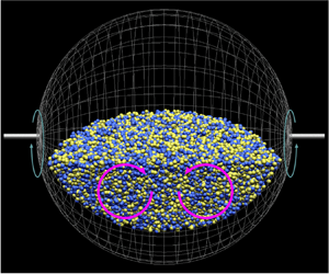
Figure 9. Temporal evolution of fluid particles initially segregated by the  $z = 0$ plane; DNS results. The filling rates are (a)
  $\varPsi =0.4$ (b)
  $0.6$ and (c)
  $0.8$. The elapsed times are (i)
  $\hat {t}/2{\rm \pi}$ = 0, (ii)
  $2.5$, (iii)
  $5$ and (iv)
  $7.5$. A supplementary movie is available at https://doi.org/10.1017/flo.2022.22.
To quantify these observations in figure 9, we introduce the degree of mixing in the container by the procedure proposed by Reference DanckwertsDanckwerts (1952). First, we divide the tracked fluid particles into two groups (groups A and B). For example, particles with an initially positive  $z$-coordinate (yellow particles in figure 9) are categorized in group A; and the others (blue particles in figure 9) are placed in group B. For simplicity, here we examine the case that the same number,
  $I$/2, of particles are assigned to each group. Next, we divide the liquid phase in the container into
  $J$ subdomains. Then, we define
  $\rho _{j}$ as the ratio of the number of group A particles to the total number of particles in the
  $j$th subdomain; and let
  $\sigma$ be its standard deviation,
 \begin{equation} \sigma = \sqrt{\frac{1}{W} \sum_{j = 1}^{J}w_j \left(\rho_{j}-\frac{1}{2}\right)^{2}},\quad W = \sum_{j = 1}^{J}w_j, \end{equation}
over all subdomains. Here,  $w_j$ denotes the volume fraction of the liquid phase in the
  $j$th subdomain. Since it is difficult to divide the liquid phase, which is surrounded by a spherical wall and the liquid–gas interface, into subdomains with a common volume, we divide the numerical domain into small cubes with an equal volume and take into account the volume fraction
  $w_j$ of the liquid phase. In terms of
  $\sigma$, the degree
  $\mathcal {M}$ of mixing is evaluated by
  $\mathcal {M}=1-2 \sigma$. Note that
  $\mathcal {M}=1$ or
  $\mathcal {M}=0$ when particles are perfectly mixed (
 $\sigma =0$) or segregated (
 $\sigma =1/2$). However, when the number of tracked particles is finite, fluctuations of
  $\rho _j$ are inevitable even in the well-mixed state. Hence
  $\mathcal {M}$ may be modified (Reference Goto, Shimizu and KawaharaGoto et al., 2014b) as
 \begin{equation} \tilde{\mathcal{M}} = \frac{1-2 \sigma}{1-2 \tilde{\sigma}}, \end{equation}
where  $\tilde {\sigma }$ is the standard deviation of
  $\rho _j$ in the perfectly mixed state. Then
  $\tilde {\mathcal {M}}=1$ for the perfect mixing, while preserving the requirement that
  $\tilde {\mathcal {M}}=0$ for the perfect segregation.
Note that  $\tilde {\mathcal {M}}$ (and
  $\mathcal {M}$) depend on the size of the subdomains and the initial categorization of particles. In this study, we define the two groups according to the
  $z$ coordinates (figure 9i) of particles’ initial positions, since it is most difficult to mix in the direction parallel to the rotation axis. The side
  $L_s$ of the cubic subdomains is set to be 1/3, 1/6 and 1/12 of the radius of the spherical container. We initially set two particles in each numerical cell for the DNS. Therefore, the total number
  $I$ of the tracked particles depends on the filling rate;
  $I \approx 1.3\times 10^7 \varPsi$. We numerically evaluate
  $\tilde {\sigma }$ in (4.3) by calculating the variance
  $\tilde {\sigma }$ for randomly distributing
  $I$ particles.
We plot the temporal evolution of the mixing degree  $\tilde {\mathcal {M}}$ in figure 10(a–c) for three different sizes
  $L_s$ and for five different
  $\varPsi$, which show that
  $\tilde {\mathcal {M}}$ increases rapidly irrespective of
  $\varPsi$ and
  $L_s$. This is consistent with the observation in figure 9. To quantify the
  $\varPsi$-dependence of the mixing performance, we define
  $T_{\tilde {\mathcal {M}}}$ by the mixing time at which
  $\tilde {\mathcal {M}}$ reaches 0.95. We plot
  $T_{\tilde {\mathcal {M}}}$ as a function of
  $\varPsi$ in figure 10(d), which shows that perfect mixing is achieved within approximately 10 spins for
  $\varPsi \lesssim 0.5$. It is also important that the mixing time is independent of
  $L_s$. This is because the small-scale vortices (figure 3) contribute to the fast small-scale mixing. In other words, the large-scale mixing, which is enhanced by the container-size vortices, determines the mixing time. The fastest mixing is achieved when
  $\varPsi$ is approximately
  $0.4$ but
  $T_{\tilde {\mathcal {M}}}$ is approximately constant (
 $T_{\tilde {\mathcal {M}}} \approx 8$) for
  $\varPsi \lesssim 0.5$. For higher filling rates (e.g.
  $\varPsi =0.8$), it takes longer times to achieve perfect mixing. However, recalling that mixing never occurs with
  $\varPsi =1$, it is important for applications that mixing occurs if the filling rate is reduced by only 0.2.

Figure 10. (a–c) Temporal evolution of mixing index  $\tilde {\mathcal {M}}$. The side of the cubic subdomains is set to be (a)
  $L_s$ =
 $1/3$, (b)
  $1/6$ and (c)
  $1/12$. (d) The number
  $T_{\tilde {\mathcal {M}}}$ of revolutions to achieve almost perfect mixing (
 $\tilde {\mathcal {M}}=0.95$) as a function of
  $\varPsi$. (e) The mean energy consumption
  $\bar {E}$ per unit time in the liquid phase for the mixing as a function of
  $\varPsi$. (
 $f$) Mixing efficiency as a function of
  $\varPsi$ in terms of (left-hand axis) the processing time
  $T_{\tilde {\mathcal {M}}}$/
 $\varPsi$ and (right-hand axis) energy consumption
  $T_{\tilde {\mathcal {M}}}\bar {E}/\varPsi$.
It may be misleading to evaluate the performance simply by  $T_{\tilde {\mathcal {M}}}$ when
  $\varPsi$ is different because we need to repeat the same operation 1/
 $\varPsi$ times to mix the liquid with the full volume of the container. Moreover, in applications, not only the time required for the mixing but also the energy efficiency are important. We define the energy dissipation per unit time
 \begin{equation} E = \int_{\varOmega_f} \phi_L \epsilon \, \mathrm{d} V,\end{equation}
to evaluate the energy required for mixing. Here,  $\epsilon =2\mu _L/\rho _L S_{ij} S_{ij}$. We plot the temporal average
  $\bar {E}$ of
  $E$ as a function of
  $\varPsi$ in figure 10(e). We can see that
  $\bar {E}$ increases up to
  $\varPsi \approx 0.6$ and decreases for
  $\varPsi \gtrsim 0.6$. As observed in figures 4(a) and 4(b), when the filling rate is low, the fluid near the wall does not follow the wall motion, i.e. the velocity gradient near the wall is large. This is the reason why the work by the container wall is large when
  $\varPsi$ is small. Although the contact area between the container wall and the liquid increases with
  $\varPsi$, the flow tends to be the solid-body rotational flow as
  $\varPsi$ approaches 1. This explains that
  $\bar {E}$ reduces when
  $\varPsi$ is sufficiently large. The
  $\varPsi$-dependence of
  $T_{\tilde {\mathcal {M}}}$ divided by
  $\varPsi$ is shown with triangles in figure 10( f) in the case
  $L_s=1/6$. This quantity corresponds to the time required to mix the liquid with the container's volume when the same mixer is used repeatedly. The fastest mixing is achieved in the case
  $\varPsi \approx 0.7$, but
  $T_{\tilde {\mathcal {M}}}/\varPsi$ is almost constant for
  $0.4 \lesssim \varPsi \lesssim 0.7$. Here, it is worth comparing the mixing ability with another existing mixer. As a representative of bladeless mixers, we recall that the precession mixer with a spherical container leads to perfect mixing of confined (
 $\varPsi =1$) fluid with approximately 10 spin revolutions (Reference Goto, Shimizu and KawaharaGoto et al., 2014b). This means that the proposed mixer takes approximately 1.5 times longer than the precessing mixer for the perfect mixing even in the fastest case (
 $\varPsi \approx 0.7$). However, we emphasize that the present mixer has a much simpler driving mechanism. The
  $\varPsi$-dependence of
  $T_{\tilde {\mathcal {M}}}/\varPsi$ multiplied by
  $\bar {E}$ is also shown with circles in figure 10( f). This quantity corresponds to the total energy consumed to mix the liquid with the container's volume. Interestingly, higher
  $\varPsi$ (
 $\varPsi \gtrsim 0.7$) is more favourable in terms of the total energy consumption.
Another method to evaluate the  $\varPsi$-dependence of the mixing ability is to use the Lyapunov exponent (Reference Kantz and SchreiberKantz & Schreiber, 2004). We have evaluated the exponent by investigating the temporal evolution of the mean distance between initially neighbouring pairs of fluid particles to confirm that the exponent is a decreasing function of
  $\varPsi$. This result supplements the
  $\varPsi$-dependence of the global mixing ability shown in figure 10(d).
In summary, the counter-rotating pair of container-size vortices (figure 4), cooperating with small-scale turbulent eddies (figure 3), enhance the mixing in all the cases of  $\varPsi$. Since the counter-rotating vortices swirl faster for lower
  $\varPsi$ (figure 5), mixing time is shorter for smaller
  $\varPsi$ (figure 10d). On the other hand, since the stronger vortices induce higher energy dissipation rates near the wall in lower
  $\varPsi$ cases, higher filling rates are more advantageous in terms of the energy consumption (circles in figure 10f).
5. Conclusion
We have discovered a new sustaining mechanism of developed turbulence of liquid, which is driven only by the steady rotation of a container. More concretely, if a spherical container is partially filled with a liquid, its steady rotation sustains turbulence, in which small-scale turbulent eddies exist – see figure 1(b–d) for experimental evidence. This phenomenon is scientifically interesting because it is quite different from the fact that the steady rotation of an any-shaped container eventually leads to the solid-body rotational flow of fluid filling it. In other words, the liquid–gas interface is essential for the sustainment of the turbulence. This phenomenon is also important for applications because, by using it, we can construct a new kind of bladeless mixer.
To understand how turbulence is driven in the container and to quantify its mixing ability, we have conducted DNS of multiphase (solid wall, liquid and gas) flow by means of the CLSVOF and BDI methods. The DNS have been validated by comparing the mean velocity with experimental data (figure 2). Then, we have demonstrated that small-scale turbulent vortices (figure 3) exist in all the cases examined in the present DNS, where the Reynolds number is high enough ( $Re=5.1\times 10^3$). It is rather important that these vortices are amplified and sustained by being stretched in shear flow around the counter-rotating pair of container-size vortices. As evidence, we show the clear coincidence between the location of the small-scale eddies (figure 3), large-scale shear flow (blue isosurfaces in figure 6) and the turbulence production term (red isosurfaces in figure 6). This means that turbulent eddies observed in the experiments (figure 1b–d) and in the DNS (figure 3) are not created by the fluctuation of the liquid–gas interface but by the shear flow around the container-size vortices (figure 4). In fact,
  $Fr(=3.6\times 10^{-3}$) is too small to deform the interface.
One of the most important observations in this flow is that the container-size pair vortices (figure 4) depend on the filling rate  $\varPsi$ of the liquid. In particular, the direction of their circulation is different depending whether
  $\varPsi$ is larger or smaller than approximately
  $0.5$. To understand the origin of this difference, we have examined in § 4.1 a numerical model, in which we drive flow, by the BDI method, just under the interface so that we can mimic the flow which is actually determined by the angle between the interface and the wall (i.e. the flow near the rotating wall). Note that the angle depends on
  $\varPsi$ (see figure 7a). This numerical model excellently reproduces the
  $\varPsi$-dependence of mean flow in the rotating sphere (figures 4 and 8). Thus, we conclude that container-size vortices stem from the flow just below the liquid–gas interface, which is driven by the flow colliding with the interface near the solid wall. It is of importance that this
  $\varPsi$-dependence of the container-size flow (figure 4) leads to
  $\varPsi$-dependencies of the turbulence production (figure 6), mean shear rate (figure 6) and the spatial distribution of small-scale vortices (figure 3).
It is therefore important to appropriately set the filling rate  $\varPsi$ when we apply this flow system to a bladeless mixer. In particular, the counter-rotating pair of container-size vortices, which plays important roles in the mixer, is stronger for
  $\varPsi \lesssim 0.5$ than
  $\varPsi \gtrsim 0.6$ (figures 4ii and 5). Though the stronger counter-rotating vortices seem appropriate for effective mixing, the smallness of the filling rate is disadvantageous when we use this system as a mixer. According to our quantification of the mixing efficiency in § 4.2 the fastest mixing is achieved when
  $\varPsi \approx 0.4$, but it is only weakly dependent on
  $\varPsi$ for
  $\varPsi \lesssim 0.5$, and almost perfect mixing is achieved with only 15 spins of the container for all the examined cases (figure 10d). We have also shown that the higher filling rates (
 $0.7 \lesssim \varPsi \lesssim 0.8$) lead to more efficient mixing in terms of the energy consumption (figure 10f).
We emphasize that the shown generation mechanism of turbulence works with large  $Re$ and small
  $Fr$. However, in the present DNS, we have only examined the cases with these parameters corresponding to our laboratory experiments (see the Appendix):
  $Re=5.1\times 10^3$ and
  $Fr=3.6\times 10^{-3}$. For actual applications as a bladeless mixer, it is important to know the
  $Re$- and
  $Fr$-dependence of the mixing ability. It is also important to investigate the dependence of the mixing ability on the container's shape. Since such an extensive parametric survey, which we are conducting by experiments and DNS, is beyond the scope of the present study, we will report results elsewhere in the near future.
Supplementary movie
Supplementary movie is available at https://doi.org/10.1017/flo.2022.22.
Acknowledgements
The DNS were conducted under the supports of the NIFS Collaboration Research Program (20KNSS145) and under the supercomputer Fugaku provided by RIKEN through the HPCI System Research projects (hp210207). We thank Professor K. Sugiyama for his advice on the numerical schemes.
Declaration of interests
The authors declare no conflict of interest.
Funding statement
This study was partly supported by JSPS Grant-in-Aids for Scientific Research (20H02068).
Author contributions
D.W. and S.G. created the research plan and wrote the manuscript. D.W. conducted all DNS.
Data availability statement
Raw data are available from D.W.
Ethical Standards
The research meets all ethical guidelines, including adherence to the legal requirements of the study country.
Appendix. Experiments
We conduct experiments by using the apparatus made for the investigation of turbulence in a precessing container (Reference Goto, Matsunaga, Fujiwara, Nishioka, Kida, Yamato and TsudaGoto et al., 2014a, Reference Goto, Shimizu and Kawahara2014b). Though the precession of the container is driven by two motors, we use one of them in the present experiments to drive the spin of a spherical container with radius 90 mm. We use a stepper motor and an accurate pulse generator to drive the spin. The container (figure 11) is made of acrylic, the outer and inner shapes of which are cylindrical and spherical, respectively. A laser sheet (with wavelength 532 nm, thickness approximately 1 mm and intensity 100 mW) runs on the equatorial plane of the spherical cavity. The working fluid is water, and we put a small amount of reflective flakes with 10–40  $\mathrm {\mu }$m major dimensions and submicron thicknesses (TiO
 $_2$-coated mica particles; see figure 1 in Reference Goto, Kida and FujiwaraGoto, Kida, and Fujiwara (2011)) to visualize fluid motions. The images shown in figure 1(b–d) were taken using a digital camera through the bottom window of the cylinder. Since the indexes of water and acrylic are not too different, we can observe flow without distortions. However, the reflection at the liquid–gas interface creates an imaginary image, which has been removed in figure 1(b–d). As shown in figure 1(b–d), we can observe complex patterns, whose characteristic length scales indicate the smallest eddy size. This implies that there exist small-scale vortices with size
  $O(10)$ mm in the sphere in all the cases with different
  $\varPsi$. This is consistent with the DNS results shown in figure 3.

Figure 11. Container used in the experiments. Its outer and inner shapes are cylindrical and spherical, respectively. We set a laser sheet on the equatorial plane and take digital images through the window at the bottom of the cylinder.
For the PIV (see figure 2) we seed nylon powders with the diameter approximately 50  $\mathrm {\mu }$m instead of the reflective flakes. We take the images using a digital camera with the frame rate 100 frames per second and use the direct correlation method to obtain the velocity field on the equatorial plane. We take the sufficiently long time average (10 spin periods) to obtain the mean velocity field (figure 2).
With the present experimental apparatus, we can accurately measure flow on the equatorial plane. However, we cannot measure flow on the  $y=0$ plane, which is essential to capture the container-size vortices (figure 4ii) because we cannot take clear images with a laser sheet on the
  $y=0$ plane due to the flange of the container (see figure 11).


 Open access