


Impact Statement
The ability to arbitrarily control the topography of a thin liquid film can be beneficial for a range of applications, from optics to biology. However, no methods exist today for achieving programmable surface deformations. This work shows that photoactuation, achieved using a low intensity projection, can effectively drive thin-film deformations via the thermocapillary effect. Furthermore, the inverse-problem approach to the thin-film equation and the analytical solutions that we present here bridge the gap between science and engineering by providing the illumination pattern required in order to produce a desired topography. Lastly, the method enables rapid prototyping of diffractive optical elements – answering an unmet need in the optical design industry.
1. Introduction
Thin liquid films are ubiquitous throughout the natural world and play important roles in a wide range of technological processes. For example, they can serve as a transport mechanism in microfluidic devices (Reference Stone, Stroock and AjdariStone, Stroock, & Ajdari, 2004), as liquid substrates for colloidal self-assembly (Reference NagayamaNagayama, 1996) or in cooling systems (Reference Kabov, Gatapova and ZaitsevKabov, Gatapova, & Zaitsev, 2008); they can also be used for fabricating optical micro-lens arrays (Reference Chronis, Liu, Jeong and LeeChronis, Liu, Jeong, & Lee, 2003; Reference Moran, Dharmatilleke, Khaw, Tan, Chan and RodriguezMoran et al., 2006) and soft robotics actuators (Reference Jones, Jambon-Puillet, Marthelot and BrunJones, Jambon-Puillet, Marthelot, & Brun, 2021), and play an important role in many biological systems such as in the lining of the lungs and eyes (Reference GrotbergGrotberg, 1994; Reference Wong, Fatt and RadkeWong, Fatt, & Radke, 1996). It is therefore of significant importance to develop robust and precise methods for controlling the behaviour of thin liquid films and for manipulating the topography of their free surface.
Several mechanisms for thin-film manipulation have been demonstrated over the past years. One such approach was demonstrated by Brown et al. who used dielectrophoretic forces produced by a set of interdigitated electrodes to create periodic deformation on the interface of a thin layer of polymer, thus solidifying them into diffraction gratings (Reference Brown, Wells, Newton and McHaleBrown, Wells, Newton, & McHale, 2009; Reference Wells, Sampara, Kriezis, Fyson and BrownWells, Sampara, Kriezis, Fyson, & Brown, 2011). Recently, Reference Gabay, Paratore, Boyko, Ramos, Gat and BercoviciGabay et al. (2021) extended this concept to allow greater control over the deformation topography using more complex electrode patterns. However, this approach requires pre-patterning of electrodes using complicated and expensive lithography processes.
An alternative actuation mechanism for manipulation of liquid interfaces is the use of the Marangoni effect, where variations in surface tension yield mass transfer across the liquid interface, resulting in its deformation. Several works demonstrated photochemical manipulation of surface tension to pattern thin polymer films (Reference Katzenstein, Janes, Cushen, Hira, McGuffin, Prisco and EllisonKatzenstein et al., 2012; Reference Kim, Janes, Zhou, Dulaney and EllisonKim, Janes, Zhou, Dulaney, & Ellison, 2015). However, similarly to the dielectrophoretic approach, photochemical manipulation of surface tension requires preparation of specialized photomasks, thus preventing arbitrary manipulation of the free surface. A potentially simpler way to induce variations in surface tension is by means of the thermocapillary effect. Numerous studies have considered the use of this approach for patterning thin polymer films (Reference SingerSinger, 2017). In particular, Nejati et al. (Reference Nejati, Dietzel and HardtNejati, Dietzel, & Hardt, 2016) leveraged the Bénard–Marangoni instability to drive short-wavelength deformation in a polymer film, yet their approach was limited to periodic structures. McLeod and Troian demonstrated deformations of nanoscale films using temperature-controlled structural elements brought in close proximity to the film, but this required the mechanical fabrication of conducting metal structures for each desired deformation (Reference McLeod, Liu and TroianMcLeod, Liu, & Troian, 2011). Programmable and dynamic freeform manipulation of liquid interfaces remains an important open problem in the thin-film community.
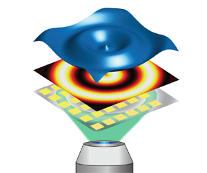
In this work, we present for the first time the use of projected light patterns as a mechanism for driving freeform deformations of a thin liquid film via the thermocapillary effect. As illustrated in figure 1, we use a standard programmable digital micromirror device (DMD) to project a desired illumination intensity map onto a substrate containing an array of light-absorbing metal pads. This provides unprecedented control over the spatial temperature distribution in the substrate, which is translated to surface tension gradients and subsequent surface deformations in the overlaying liquid film. We derive a theoretical model for an inverse problem that provides the required temperature map for achieving a desired topography. When using a curable polymer, the resulting topography can be solidified to create specially designed molecularly smooth surfaces. The entire shaping and curing process is completed in under 5 min, and the same light-absorbing substrate can be used again to create a different topography using a new projected pattern.

Figure 1. Operational principle of the thermocapillary fluidic shaping method. (a) Schematic illustration of the experimental set-up. The set-up is based on a shallow fluidic chamber filled with a thin layer of a curable polymer. The bottom surface of the chamber is a glass substrate patterned with an array of metal pads designed to absorb light in the visible spectrum. A desired illumination pattern is projected onto the surface using a DMD-based system. The inset describes the internal structure of the metallic pads. (b) A desired illumination pattern is projected onto the metal pads, which absorb the light and create a corresponding temperature field. Heat is transferred from the pads, through the thin liquid layer and to the liquid–air interface, leading to surface tension gradients that drive the thermocapillary effect, resulting in spatial deformations of the free surface. (c) Image of the solidified polymer after exposure to UV illumination.
We chose to demonstrate the applicability of our method for rapid prototyping of freeform diffractive optical elements (DOEs). The DOEs are used to manipulate light by introducing non-uniform phase accumulation through a carefully designed geometry and/or by changing the refractive index of the optical element (Reference Born and WolfBorn & Wolf, 2013), and are key components a in a wide range of optical applications (Reference Turunen and WyrowskiTurunen & Wyrowski, 1998). The DOEs are typically created using clean room fabrication techniques, such as direct writing, focused ion beam milling, grey scale lithography and interferometric exposure (Reference O'Shea, Suleski, Kathman and PratherO'Shea, Suleski, Kathman, & Prather, 2004) or by precise multi-axis mechanical processes such as diamond machining or magnetorheological finishing (Reference KordonskiKordonski, 2011; Reference Rolland, Davies, Suleski, Evans, Bauer, Lambropoulos and FalaggisRolland et al., 2021). However, all of these processes require significant and expensive infrastructure and highly skilled operators, which lowers accessibility and drives high component costs. Furthermore, existing techniques do not allow for rapid prototyping, which is much desired for driving research and design innovation.
Here, using the inverse-problem approach, we first demonstrate the fabrication of a one-dimensional diffraction grating component and characterize its performance, showing good agreement with theory. We then demonstrate the fabrication of an axisymmetric phase mask for extended depth of focus (EDOF) and show its implementation in imaging over a greater focal depth without reducing the numerical aperture. Finally, we demonstrate the fabrication of a non-axisymmetric saddle-point phase mask (Reference Shechtman, Sahl, Backer and MoernerShechtman, Sahl, Backer, & Moerner, 2014), and experimentally demonstrate its use in encoding of depth information in the point spread function (PSF) of nanoparticles, allowing microscopic three-dimensional particle tracking (Reference Ferdman, Ferdman, Nehme, Nehme, Weiss, Orange and ShechtmanFerdman et al., 2020). We provide complete details of the experimental system, and characterize its resolution and dynamic range as a function of the illumination intensity and of the absorbing array geometry. Our method thus provides a potential solution for low-cost customized fabrication of DOEs for industrial applications, and allows for rapid prototyping of new DOE-based ideas in research.
2. Results
2.1 Principles of the method
Figure 1 presents the principle of operation of the thermocapillary fluidic shaping method and the experimental set-up used for its implementation. When localized heating is imposed on a gas–liquid interface, the liquid will flow outward along the free surface from warmer regions with lower surface tension to colder regions with higher surface tension. This results in local deformation of the liquid film (Reference Tan, Bankoff and DavisTan, Bankoff, & Davis, 1990), and is known as the thermocapillary effect. The magnitude of the surface deformation is proportional to the local temperature gradients. We found that a convenient way to control these temperature gradients is to use light projection, whose spatial intensity can be easily programmed, to heat an array of absorbing metal pads patterned on the bottom of the fluidic chamber. The system uses a standard <3 W microscope light emitting diode (LED) source and a standard DMD. The resulting increase in temperature is of the order of few degrees or less, and is sufficient to drive significant deformations.
The spatial resolution of the thermal patterning depends on the material properties of the substrate, the resolution of the projected pattern and the geometry of the light-absorbing metallic pad array. The composition of the metal pads was designed to maximize light absorbance across the ultraviolet-visible (UV-Vis) spectrum of the light source, as shown in figure 1(c). Section 2 in the supplementary movie and material available at https://doi.org/10.1017/flo.2022.17 provides characterization of the deformation magnitude and resolution in our system as a function of the illumination intensity and pad array density. As expected, the magnitude of the resulting deformation is proportional to both the illumination intensity and the area fraction occupied by the pads. The precise deformation magnitude and resolution depend on the specific heating pattern, with some tradeoff between the two (see the theory section). However, typical values are of the order of 3 μm maximum deformation and 5 μm mm−1 spatial resolution.
2.2 The inverse problem − theory and implementation
Consider an open microfluidic chamber of length  $\mathrm{{\cal L}}$, containing a thin liquid film of thickness
  ${h_0}$, as depicted in figure 1(a). The chamber is heated from below by a light pattern that is absorbed by the metal pads array, resulting in temperature variations over a characteristic length l,
  ${h_0} \ll l \ll \mathrm{{\cal L}}$. For small variations in temperature, we can assume that the surface tension,
  $\sigma $, changes linearly with temperature,
  $\theta $, according to
 \begin{equation}\sigma = {\sigma _r} - \beta (\theta - {\theta _r}),\end{equation}
where  $\beta \equiv \partial \sigma /\partial \theta $ is defined as the thermocapillary coefficient and is assumed to be constant,
  ${\theta _r}$ is a reference temperature and
  ${\sigma _r}$ is the surface tension at that temperature. We assume that variations in temperature are sufficiently small such that changes in density and viscosity are negligible.
In supplementary material § 3 we provide a complete derivation of the governing equations. Briefly, we consider the continuity equation, the steady-state incompressible Navier–Stokes equations and the steady-state advection–conduction heat equation. At the bottom of the film  $(z = 0)$ we require no-slip and no-penetration conditions on the flow, and set a fixed temperature distribution,
  ${\theta _b}$. At the liquid--air interface
  $(z = h(x,y))$ we impose the kinematic condition relating flow velocities to the shape of the deformed interface, a stress balance relating the stress tensor in the liquid to surface tension and heat loss through Newton's cooling law. Using these equations and boundary conditions, we derive the dimensionless steady-state equation of the deformed liquid film driven by a non-uniform temperature distribution
 \begin{equation}{\boldsymbol{\nabla} _2} \boldsymbol{\cdot} \left[ {\frac{S}{3}{H^3}{\boldsymbol{\nabla}_2}\nabla_2^2H - \frac{G}{3}{H^3}{\boldsymbol{\nabla}_2}H - \frac{1}{2}{H^2}{\boldsymbol{\nabla}_2}\left( {\frac{{{\vartheta_b} + \varTheta }}{{1 + BH}}} \right)} \right] = 0.\end{equation}
Here,  $[X,Y,Z,H] = [x/l,y/l,z/{h_0},h/{h_0}]$ are the dimensionless coordinates and film thickness scaled by the characteristic lateral and vertical dimensions, and
  ${\boldsymbol{\nabla} _2} = (\partial /\partial X,\partial /\partial Y)$ and
  $\nabla _2^2 = ({\partial ^2}/\partial {X^2} + {\partial ^2}/\partial {Y^2})$ are the two-dimensional gradient and Laplacian operators. We scale the velocity as
  $[U,V,W] = (1/{U_0})[u,v,(1/\varepsilon )w]$, where
  $U_0 = \varepsilon \mathrm{\Delta }\sigma/\mu $ is the characteristic velocity as derived from the tangential stress balance, with
  $\Delta \sigma = \beta \Delta \theta $ being the characteristic variation in surface tension, and
  $\mathrm{\Delta }\theta = {\theta _{{b_{max}}}} - {\theta _{{b_{min}}}}$ the difference between the maximum and minimum temperatures at that surface. Also,
  $\mu $ is the dynamic viscosity of the liquid, and
  $\varepsilon = {h_0}/l \ll 1$ is the ratio of film thickness to characteristic lateral scale. We scale the temperature as
  $\vartheta = (\theta - {\bar{\theta }_b})/\mathrm{\Delta }\theta $, where
  ${\bar{\theta }_b}\; $is the average temperature of the bottom surface,
  $S = {\varepsilon ^3}({\sigma _r}/\mu {U_0}) = {\varepsilon ^2}({\sigma _r}/\mathrm{\Delta }\sigma )$ is the surface tension number
  $B = {{\mathscr{h}}h_{0}}/{k}$ is the Biot number,
  ${\mathscr{h}}$ is the heat transfer coefficient at the liquid–air interface, k is the thermal conductivity,
  $\varTheta = ({\bar{\theta }_b} - {\theta _\infty })/\mathrm{\Delta }\theta $ is a ratio of temperature differences, where
  ${\theta _\infty }$ is the ambient temperature, and
  $G = \varepsilon (\rho h_0^2/\mu {U_0})g = (\rho h_0^2/\mathrm{\Delta }\sigma )g$ is the dimensionless gravity.
Subjected to appropriate boundary conditions on the thickness of the liquid film (e.g. far from the heating region, the film thickness can be assumed to be known and uniform), (2.2) can be solved numerically to obtain a solution to the direct problem − the spatial deformation resulting from any prescribed temperature distribution  ${\vartheta _b}(x,y)$. However, for engineering purposes, the inverse problem − seeking the temperature map that would yield a desired deformation − is of greater value.
We approach the inverse problem by first considering the one-dimensional case described by
 \begin{equation}\; \; \; {\partial _\textrm{X}}\left[ {\frac{S}{3}{H^3}\partial_X^3H - \frac{G}{3}{H^3}{\partial_\textrm{X}}H - \frac{1}{2}{H^2}{\partial_X}\left( {\frac{{{\vartheta_b} + \varTheta }}{{1 + BH}}} \right)} \right] = 0,\end{equation}
where X is the non-dimensional spatial coordinate. We assume that the temperature variations occur far from the boundaries,  $X ={\pm} \mathrm{{\cal L}}$, and therefore at the boundaries the film can be assumed to be flat
 \begin{equation}H({\pm} \mathrm{{\cal L}}) = 1,\quad \partial _X^nH({\pm} \mathrm{{\cal L}}) = 0\{ n = 1,2,3\} ,\quad {\vartheta _b}({\pm} \mathrm{{\cal L}}) = {-} \varTheta ,\quad {\partial _X}{\vartheta _b}({\pm} \mathrm{{\cal L}}) = 0.\end{equation}
 Integrating equation (2.3) in X and dividing by  ${H^2}$ we obtain
 \begin{equation}\frac{S}{3}H\partial _X^3H - \frac{G}{3}H{\partial _X}H - \frac{1}{2}{\partial _X}\left( {\frac{{{\vartheta_b} + \varTheta }}{{1 + BH}}} \right) = \frac{{{C_0}}}{{{H^2}}},\end{equation}
where  ${C_0}$ is an integration constant. The left-hand side can be integrated by parts, and vanishes when using the boundary conditions (2.4a–d)
 \begin{equation}\int_{ - \mathrm{{\cal L}}}^\mathrm{{\cal L}} {\left[ {\frac{S}{3}H\partial_X^3H - \frac{G}{3}H{\partial_\textrm{X}}H - \frac{1}{2}{\partial_X}\left( {\frac{{{\vartheta_b} + \varTheta }}{{1 + BH}}} \right)} \right]\,\textrm{d}X = 0} .\; \end{equation}
 Since the integration of the right-hand side of (S4) is non-zero, the coefficient  ${C_0}$ must vanish,
  ${C_0} = 0$.
The one-dimensional steady state (2.5) can thus be simplified to
 \begin{equation}\frac{S}{3}H\partial _X^3H - \frac{G}{3}H{\partial _X}H - \frac{1}{2}{\partial _X}\left( {\frac{{{\vartheta_b} + \varTheta }}{{1 + BH}}} \right) = 0.\end{equation}
Integrating equation (2.7) to an arbitrary position  $\xi $ yields an explicit expression for the temperature variation,
  ${\theta _b}(\xi )$, required in order to create the desired deformation
  $H(\xi )$:
 \begin{equation}{\vartheta _b}(\xi ) = \frac{{1 + BH(\xi )}}{3}[2SH(\xi )\partial _\xi ^2H(\xi ) - S{({\partial _\xi }H(\xi ))^2} - G(H{(\xi )^2} - 1)] - \varTheta .\end{equation}
The two-dimensional case cannot be directly integrated. We therefore propose an ansatz based on the one-dimensional solution
 \begin{equation}{\vartheta _b} = \frac{{1 + BH}}{3}[2SH{\nabla ^2}H - S{(\boldsymbol{\nabla }H)^2} - G({H^2} - 1)] - \varTheta .\end{equation}
As detailed in the supplementary movie and material, by substituting (2.9) into the governing equation (2.2), we obtain the difference between the approximate (ansatz) solution and the exact solution
 \begin{equation}\boldsymbol{\epsilon } = \frac{S}{3}[({\partial _Y}H\partial _{XY}^2H - {\partial _X}H\partial _Y^2H),({\partial _X}H\partial _{XY}^2H - {\partial _Y}H\partial _X^2H)].\end{equation}
 The ansatz solution is thus exact when the non-normalized Gaussian curvature of the surface,  $K = \partial _X^2H\partial _Y^2H - {(\partial _{XY}^2H)^2}$, vanishes. For other surfaces, the error would depend on the magnitude of the Gaussian curvature, and we provide a numerical assessment for this error in supplementary material § 3.
Figure 2 presents the use of the inverse problem for fabricating a desired topography. Figure 2(a) presents the prescribed topography composed of a set of concentric rings, with a maximum deformation relative to the baseline film thickness of  $d_{desired} = 1.5\;\mathrm{\mu }\textrm{m}$. This topography is used as input into (2.3), with the constant parameters as defined in supplementary material § 4, resulting in a temperature distribution
  ${\vartheta _b}(x,y)$. Since we do not have a direct relation between the desired temperature and the required illumination intensity, we assume a linear dependence and perform a calibration measurement in which the illumination intensity map is set to
  $I(x,y) = {I_0}\; {\vartheta _b}(x,y)/\; \textrm{max}\{ {\vartheta _b}(x,y)\} $, where
  ${I_0}$ is the maximum intensity of the light source. The resulting intensity map is presented in figure 2(b), and an image of the actual projected intensity map is presented in figure 2(c). We measure the resulting maximum deformation,
  ${d_{max}}$ (which for this pattern was 2.2 μm), and repeat the projection using an intensity map that is scaled by
  ${d_{desired}}/{d_{max}}$ (i.e. 1.5/2.2). Figure 2(d) presents the resulting topography of the (solidified) deformed liquid film. There is a good qualitative agreement between the desired pattern and the resulting one yet deviations are also clearly visible. We further discuss these deviations in the Conclusions section.

Figure 2. Demonstration of a complete workflow for an inverse-problem solution. (a) The desired topography defined in terms of the variation from a reference height. (b) The intensity map required in order to produce the desired deformation, as obtained from solving the inverse problem. (c) Image of the illumination pattern as obtained on the bottom surface of the fluidic device. (d) The resulting topography after curing the polymer as measured by the DHM (Reference Cuche, Marquet and DepeursingeCuche, Marquet, & Depeursinge, 1999).
2.3 Applications
Figures 3–5 present several practical diffractive elements produced using the thermocapillary fluidic shaping approach. Diffraction gratings are optical elements with a periodic structure, that diffract the incident light into several beams traveling in different directions, depending on the wavelength and the spatial periodic structure defining the angular spread. They are commonly used in monochromators for spectroscopic instruments (Reference Loewen and PopovLoewen & Popov, 2018).
Figure 3 presents a linear diffraction grating with a peak-to-peak periodicity of 400 μm produced by projection of a sinusoidal illumination pattern. Figure 3(a) presents the projected pattern side by side with the resulting deformation, and figure 3(b) presents the magnitude of the deformation along the centreline. We test the resulting element by measuring the diffractive angle for several wavelengths produced by monochromatic LEDs. Since the LEDs have a spectral bandwidth of approximately 50 nm, we use a weighted average of their spectrum (as provided by the manufacturer) to define a representative wavelength for the analysis. As shown in figure 3(c), the results are in excellent agreement with the expected angle set by the element's periodicity. Figure 3(d) also presents a visual demonstration of white light diffracted through the grating and directly imaged by a camera sensor, clearly showing the separation of bands.

Figure 3. Fabrication and testing of a linear diffraction grating. (a) Side-by-side image showing the projected light pattern (left) and the measured resulting topography (right). Regions with a higher projected intensity, and therefore a higher temperature, correspond to valleys in the topography. (b) The deformation magnitude along the centre of the element, showing the spatial frequency (400  $\mu$m) and the resulting amplitude (0.4
  $\mu$m) of the grating. (c) The measured diffractive angle for three wavelengths passing through the grating. The reciprocal of the slope of a least-square line matches well the designed grating spatial frequency. (d) Image of white light diffraction. The numbers along the scale indicate the centre of each band along a horizonal centreline.
The depth of field of any optical system can be extended by reducing its numerical aperture, yet at the cost of reducing the amount of light collected. A number of studies have shown the ability to overcome this limitation and extend the depth of field without loss of photons, by positioning an appropriate phase mask in the systems’ aperture (Reference Ben-Eliezer, Marom, Konforti and ZalevskyBen-Eliezer, Marom, Konforti, & Zalevsky, 2005; Reference Dowski and CatheyDowski & Cathey, 1995). Figure 4 presents the fabrication and testing of an extended depth of focus (EDOF) phase mask designed by formulating a phase retrieval task as described by Nehme et al. (Reference Nehme, Ferdman, Weiss, Naor, Freedman, Michaeli and ShechtmanNehme et al., 2021). The desired mask mould is translated into a light pattern (figure 4b) using the inverse-problem solution, and the thermocapillary fluidic shaping method is used to create a solid mould. We then cast Polydimethylsiloxane (PDMS) onto the mould to create the phase mask itself, shown in figure 4(c). We position the mask in the Fourier plane of a 4f system and use it to image three targets positioned at different distances from the camera. As illustrated in figure 4(d), to ensure that the presence of the mask itself does not reduce the numerical aperture, we use a smaller fixed aperture in close proximity to the mask, acting as the aperture stop of the system. Figures 4(e) and 4(f) clearly show the additional depth of field gained by using the mask, yet with some loss of contrast.

Figure 4. Fabrication and demonstration of an extended depth of field phase mask. (a) The design of the EDOF mask based on Nehme et al. (Reference Nehme, Ferdman, Weiss, Naor, Freedman, Michaeli and ShechtmanNehme et al., 2021). (b) The projection pattern for a negative mould, as solved by the inverse problem. (c) The obtained phase mask as measured by the DHM. (d) Schematic illustration of the optical set-up. We position the phase mask in the Fourier plane of a 4f system, and image three targets positioned 2.5 cm from one another. We used an additional small fixed aperture to ensure that the phase mask itself does not reduce the aperture stop. (e) The resulting image without the phase mask, showing only the centre target in focus. (f) The resulting image with the EDOF phase mask showing all three targets in focus.
Three-dimensional localization microscopy uses phase masks positioned in the Fourier plane of a microscope to modify the PSF in order to encode three-dimensional information (Reference Pavani, Thompson, Biteen, Lord, Liu, Twieg and MoernerPavani et al., 2009). Figure 5 presents the use of the inverse-problem approach for fabrication of such a phase mask. Figure 5(a) presents the topography of the desired ‘tetrapod’ mask (Reference Shechtman, Sahl, Backer and MoernerShechtman et al., 2014), designed to provide depth information over a range of ±2 μm. Here, too, we use the desired mould topography as input to (2.3) and obtain the intensity map presented in figure 5(b). The parameters used in the solution are identical to those that were used in figure 4 and that are detailed in supplementary material § 3. Figure 5(c) presents the topography of the resulting phase mask created by casing PDMS onto the resulting mould, as measured by the digital holographic microscope (DHM). The first column in figure 5(d) presents the measured PSF of a single emitter (a 200 nm fluorescent bead) at different locations along the optical axis, in the absence of any phase mask. The second column presents the measured PSF of the same emitter, when using a phase mask produced using a 3-step lithography process. The last column in figure 5(d) presents the measured PSF as obtained using our phase mask fabricated by the thermocapillary fluidic shaping method. Figure 5(e) demonstrates the use of this mask for three-dimensional tracking of three 200 nm beads undergoing Brownian motion (see supplementary movie 1 and material) in a liquid environment, and of one stationary bead (attached to the bottom surface).

Figure 5. Fabrication and demonstration of a saddle-point phase mask for three-dimensional localization microscopy. (a) Topography map of a saddle-point phase mask microfabricated using standard lithography and ion etching processes. (b) The illumination pattern required for deforming the liquid film into a negative mould for the phase mask, as obtained from the inverse-problem solution. (c) The DHM measurement of the resulting solidified PDMS mask, cast on the mould fabricated by thermocapillary fluidic shaping. (d) The PSF of a 200 nm diameter fluorescent microsphere at various z positions, as obtained from (i) a measured standard PSF with no phase mask (ii) a measured PSF using a lithography phase mask, (iii) a measured PSF using the mask obtained through thermocapillary fluidic shaping. (e) Tracking of three nanobeads undergoing Brownian motion and one stationary bead (in green) in a liquid, using the fabricated mask.
4. Conclusions
In this work, we introduced a novel method for thermocapillary shaping of thin polymer films, and applied it as means for the rapid fabrication of DOEs. We provided a theoretical model for the inverse problem, making it possible to design specific topographies corresponding to desired optical functionalities. This approach has several significant advantages over existing fabrication technologies. First and foremost, the method is programmable in the sense that the desired deformation is created in response to the projected pattern. Thus, a single set-up can be used to implement a wide range of different designs. For the film thickness used in our work, and for the typical topographies presented here, the steady-state shape of the liquid film is formed in a matter of seconds. Once the liquid element is exposed to UV light, it undergoes rapid solidification and results in a molecularly smooth solid element. Complete polymerization is usually achieved in less than a minute; however, for extra margins, we exposed the films to UV for approximately 5 min. The short fabrication time scale makes the method especially attractive for rapid prototyping of DOEs, allowing maximal flexibility for testing various optical designs. To illustrate the utility of the method, we fabricated several DOEs and demonstrated their functionality.
Using our current set-up, we were able to achieve deformations of the order of several microns over a lateral span of millimetres. The magnitude of deformations is sufficient for most applications in the visible spectrum, as it allows for phase accumulation of at least 2π. The deviations between the desired profiles and the experimentally obtained ones can be attributed to a number of factors. These include accuracy in levelling of the fluidic chamber, non-uniformities in the illumination source, non-uniformity in the height of the boundary, additional heat convection due to air currents in the laboratory or contamination of the liquid interface (e.g. surfactants, dust). Future development of this technique should account for these issues in constructing the experimental set-up. In the relatively thick films considered here, spatial resolution is limited by the natural heat convection from the liquid film. Higher spatial resolution could potentially be achieved by working with thinner films, as was previously demonstrated in other works on Marangoni-based patterning (Reference Katzenstein, Janes, Cushen, Hira, McGuffin, Prisco and EllisonKatzenstein et al., 2012; Reference Kim, Janes, Zhou, Dulaney and EllisonKim et al., 2015). Additional techniques such as effective heat removal and precisely controlled ambient temperature, will also aid in increasing the spatial resolution of the method.
Our inverse-problem solution provides the temperature distribution required for a desired deformation. In our implementation, we assume a linear relation between the desired temperature and the projected light intensity. However, this assumption must be verified, and may be an additional source of deviation between the desired and obtained topographies. More generally − an empirical model relating the temperature to projection intensity should ideally be created. To do so, the temperature on the liquid interface should be measured, requiring high resolution and high precision thermal imaging. Alternatively, the topography of the liquid film could be measured in real time (e.g. by interferometry) allowing us to close a loop and modify the projection pattern dynamically to match the desired shape before the element is solidified. Another attractive feature of this approach is the simplicity and affordability of the required set-up, consisting of a simple projector and a reusable substrate containing an array of light-absorbing metal pads. As such, this technology can be easily scaled up and implemented in any laboratory, allowing for low-cost customized fabrication of DOEs for both research and industrial applications.
Finally, while in this work we focused on fabricating solid topographies, the shape of the liquid interface can be dynamically controlled by varying the projected light in real time. This capability suggest that the method presented here could potentially be applied to fields such as adaptive optics, colloidal assembly and manipulation of cells and particles in the biomedical sciences.
Acknowledgements
We thank B. Rofman for performing the atomic force microscopy measurements for surface roughness characterization.
Funding statement
This project has received funding from the European Research Council (ERC) under the European Union's Horizon 2020 Research and Innovation Programme, grant agreement no. 678734 (MetamorphChip).
Competing interests
The authors declare that they have no competing interests.
Data availability statement
All relevant data are contained within the manuscript.
Ethical standards
The research meets all ethical guidelines, including adherence to the legal requirements of the study country.
Author contributions
V.F. and M.B. conceived the method. R.E. developed the experimental set-up, performed the thermocapillary experiments, collected and analysed the data. V.F. and M.N. developed the theory. R.E., V.F., O.L., M.N. and M.B. designed the experiments. O.L. designed and simulated the light absorption layer. K.G. fabricated the devices. M.S. designed and built the digital mirror device module. Y.S. conceived the optical experiments. B.F. designed the phase masks. R.E. and N.O. designed and performed the three-dimensional localization experiments. R.E. and M.B. wrote the manuscript. All authors reviewed and commented on the manuscript.
Supplementary movie and material
Supplementary material document and supplementary movie intended for publication have been provided with the submission. These are available at https://doi.org/10.1017/flo.2022.17.
Appendix A: Methods and materials
A.1 Thermocapillary shaping experimental set-up
The experimental set-up consists of a glass substrate patterned with metallic pads fabricated by liftoff photolithography processes. The pads consist of two metallic layers − a 150 nm chromium layer, followed by a 50 nm gold layer. The metal pads were then coated with a 400 nm silicon dioxide layer to protect them. We used polyvinyl chloride tape to form the boundaries of a 2 cm × 2 cm × 60 μm fluidic chamber on top of the patterned substrate. Before filling the fluidic chamber, we treated the device with low-pressure air plasma (Zepto W6, Diener Electronics, Germany) for 1 min, allowing for improved wetting of the substrate. Next, we injected ~15 ul of a UV curable polymer (CPS 1050 UV, Colorado Photopolymer Solutions, USA) to fill the chamber. We covered the chamber with a UV-transparent polystyrene lid to protect the polymer from contamination. The illumination system (depicted in figure 1) consists of a liquid guide connected to a computer-controlled LED light source (Sola SE, Lumencore, USA) and a beam expander composed of two lenses: L1, an aspherical condenser (ACL25416U-A, Thorlabs, USA); and L2, a biconvex lens (LB1723-A, Thorlabs, USA) to magnify the beam. We collimate the light into a digital mirror device (1024 × 768 pixels, V7001, Texas Instruments, USA), allowing the projection of any desired shape. The projected light passed through L3, a Kohler lens with f = 300 mm (AC254-300-A, Thorlabs, USA), which focuses the light onto the back focal plane of the microscope objective (PlanApo, 10x, NA = 0.45, Nikon, Japan). To create a desired deformation, we illuminate the bottom of the device with a corresponding light pattern and allow 1 min for equilibration. We then position the UV lamp (24 W, emission wavelength λ = 370 nm) at a distance of ~20 mm above the substrate and illuminate for 4 min to cure the polymer into a solid element. We measure the topography of the resulting components using a digital holographic microscope (DHMR1003, LynceeTec, Switzerland).
A.2 Fabrication of PDMS based DOEs
We fabricated our DOEs by casting Polydimethylsiloxane (PDMS) at a ratio of 1 : 10 (cross-linker to resin) on top of the solidified UV polymer, after treating the polymer surface with Chlorotrimethylsilane (Sigma Aldrich, Germany). After casting the PDMS, we placed the mould in a vacuum chamber for 3 h for degassing, followed by 3 h at 60 °C in the oven for curing.
A.3 Engineered PSF measurement and bead tracking
We placed the PDMS phase mask in the Fourier plane of a 4f system, located on the imaging exit of an inverted microscope (Ti2, Nikon, Japan) equipped with a ×100 objective (CFI SR HP Plan Apochromat Lambda S 100XC Sil, Nikon, Japan). To create the reference z-stack, we deposited 200 nm diameter fluorescent emitters (TetraSpeck, Thermo Fisher, USA) on a glass slide and excited them with a combination of a 488 nm and 532 nm lasers. We then imaged the PSFs of the optical system containing the tetrapod phase mask, as a function of the z coordinate of the beads over an axial range of 4.5 μm with steps of 50 nm. The z-stack was used to estimate the optical system's pupil function using phase retrieval (Reference Ferdman, Ferdman, Nehme, Nehme, Weiss, Orange and ShechtmanFerdman et al., 2020).
We then placed the same type of beads in a water–glycerol mixture, allowed to move freely under Brownian motion, and imaged them using the tetrapod phase mask. We then used the z-stack to retrieve their three dimensional coordinates, using a maximum likelihood estimation, per frame.
A.4 Diffraction grating measurement
To measure the diffraction through the fabricated grating, we transmitted collimated monochromatic light through the grating and measured the diffraction pattern on a camera sensor (D90, Nikon, Japan) located at a distance of 1 m. We repeated this using three different LED sources (M660F1, M530F1, M470F1, Thorlabs, USA) with spectral peaks at 660 nm, 530 nm and 470 nm. The three LEDs were fibre coupled, allowing the use of a single collimation set-up, and switching of the light sources by connecting the fibre input to the different sources. The collimation set-up was based on an aspheric condenser (ACL25416U-A, Thorlabs, USA) focused onto a 50 μm pinhole, and ×2 objective (Plan UW, NA 0.06, Nikon, Japan) for collection of the light.
A.5 EDOF measurement
The imaging set-up is presented in figure 5(d). The 4f imaging system consists of two lenses, L1 (AC254-100-A, Thorlabs, USA) and L2 (AC254-250-A, Thorlabs, USA), and a monochromatic CCD sensor. The phase mask was placed at the Fourier plane of the system, and an aperture was located adjacent to it. In the reference experiment, the phase mask was removed, but the aperture was maintained, to ensure the same aperture stop for both cases. The imaged target consisted of three of three ~5 mm printed figures connected to a ruler and located at distances of 247.5 mm, 250 mm, and 252.5 mm from the L2 lens.


 Open access