


1 Introduction
Survivor funds are investment pools where participants’ contributions are re-distributed ex-post, according to the mortality experienced by the group. Precisely, participants agree to share the proceeds of a collective investment pool favoring those who survive in application of a specified mutual inheritance rule. The latter boosts the performance of investments, making survivor funds particularly attractive because of their greater return. Survivor funds are named after Forman and Sabin (Reference Forman and Sabin2016). Several variants exist and they are also known under various appellations, such as individual tontine accounts (Fullmer and Sabin, Reference Fullmer and Sabin2019) or pooled-survival funds (Newfield, Reference Newfield2014), for instance.
Survivor funds run over one period of time. The latter is henceforth referred to as the reference period. According to the agreed mutual inheritance rule, the initial contributions are lost in case of death during the reference period. Mortality credits correspond to the decedents’ contributions and are shared among all participants (to reward them for having put their contribution to the fund at risk of being lost in case of death during the reference period). Precisely, survivors get financial return plus mortality credits generated by the mutual inheritance rule, while decedents lose their initial contribution but their beneficiaries still receive mortality credits. Even if no participants die, survivors never get less than the return on the underlying investment. The way mortality credits are distributed must account for the possibly unequal death probabilities and contributed amounts. In that respect, participants assuming more risk, because of higher death probability or higher amount of contribution, should receive a higher share of these credits.
Survivor funds are currently offered by Le Conservateur in France. Founded in 1844 and established as a mutual insurance association (under the brand name “Les Associations Mutuelles Le Conservateur”), the aim was to develop and modernize the tontine mechanism created by Italian banker Lorenzo Tonti in 1653. Survivor funds proposed by Le Conservateur are described on their website (see www.conservateur.fr/nos-produits/tontine/). Each year, a new tontine association is created for the next 25 years. Participants can enroll for that duration, or join an existing tontine if they prefer a shorter duration. Contributions can thus be invested in the long term. At maturity, the proceeds of the collective investment pool are distributed according to a predefined rule taking into account participant’s age and amount invested. The present paper aims to study the way mortality credits are shared, as well as their behavior in large pools.
Within a homogeneous group (in terms of mortality and amount of contribution), it suffices to distribute mortality credits uniformly over all participants, so that each of them receives an equal share of the total amount of decedents’ contributions. However, the restriction to homogeneous groups limits the number of participants which inevitably increases the volatility of the final payout. Allowing for heterogeneity in death probabilities and contributed amounts avoids this drawback and makes the participation in such investment more attractive (especially at old ages), provided mortality credits are shared in an understandable, acceptable and transparent way.
Several proposals for mutual inheritance schemes have been made in the literature, see for example Donnelly and Young (Reference Donnelly and Young2017). Denuit (Reference Denuit2019) proposed to adopt the conditional mean risk sharing rule introduced in Denuit and Dhaene (Reference Denuit and Dhaene2012) to share mortality credits among participants within a survivor fund. This rule extends the uniform allocation rule applying within homogeneous groups to heterogeneous situations, where participants differ in terms of mortality and/or amounts of invested assets. According to this rule, each participant receives the conditional expectation of the individual account value, given the total mortality credits experienced by the entire pool. Calculations are carried out as if we knew beforehand the total value of mortality credits to be distributed over the entire pool, but not who actually died. The expected value of the invested amount lost by each participant in case of death is then computed, given each possible realization of total mortality credits. Explained differently, each participant gets the average share of mortality credits corresponding to his or her risk profile so that participants with higher death probabilities or larger amounts of investment get a comparatively larger share of mortality credits.
The conditional mean risk sharing rule satisfies the risk exchange fairness condition and enjoys many theoretical properties (Denuit, Reference Denuit2020, Denuit and Robert, Reference Denuit and Robert2021a,d). Mortality credits provided by survivor funds improve in convex order when the size of the pool increases. This ensures that the variance of mortality credits decreases when the number of participants gets larger while their expected value stays constant, whatever the individual death probabilities and initial contributions as long as participants’ lifetimes are mutually independent and the sharing is operated according to the conditional mean risk allocation rule. This paper shows that the variance of mortality credits tends to zero when the size of the group tends to infinity provided the amounts contributed by participants satisfy some mild assumptions. This means that individual risk can be fully diversified within infinitely large pools under the conditional mean risk sharing rule. Some simple, hierarchical approximations are proposed for mortality credits within large pools.
Survivor funds are fixed-term investment vehicles operating in a one-period setting, as opposed to the multi-period analysis developed in modern tontines or pooled annuity funds. It is nevertheless possible to generate lifelong incomes by investing in survivor funds over successive time intervals. This offers an alternative to group self-annuitization schemes of Piggott et al. (Reference Piggott, Valdez and Detzel2005) as well as to modern tontines or pooled annuity funds developed for example by Bernhardt and Donnelly (Reference Bernhardt and Donnelly2021), Chen et al. (Reference Chen, Qian and Yang2021), and Hieber and Lucas (Reference Hieber and Lucas2022).
Modern tontines receive a lot of interest these days. They offer many advantages compared to classical retirement products. See for example Winter and Planchet (2021) as well as the practical solutions designed by the pensiontech Nuovalo Ltd ( www.nuovalo.com ). The present paper proposes an alternative to generate lifelong incomes by investing accumulated savings at retirement in survivor funds running over several periods. Decomposing the pooled annuity fund into a sequence of survivor funds is also more transparent, allowing participants to keep control of the remaining part of their assets, and eases investment policies since each survivor fund operates over a fixed time horizon. To end with, let us notice that the results derived in this paper are also useful for death benefits, when participants contribute ex post in function of premature deaths. A similar concept was successfully introduced by Xianghubao, a mutual aid platform in China. Here, payments are not triggered by death but by a critical illness diagnosis, see also Abdikerimova and Feng (Reference Abdikerimova and Feng2022).
The remainder of this paper is organized as follows. In Section 2, we recall the definition of survivor funds and apply the conditional mean risk sharing rule to allocate mortality credits to each participant. Section 3 establishes the behavior of individual mortality credits within large pools when participants are subject to different death probabilities but contribute the same amount (heterogeneity in mortality but homogeneity with respect to invested contributions). It is demonstrated that the variance of mortality credits decreases with the size of the group, tending to zero when the number of participants tends to infinity so that individual risk can be fully eliminated at the limit under the conditional mean risk sharing rule. It is also shown how to supplement the system with minimum guarantees. Section 4 allows for different amounts of contribution selected from a predefined menu. Imposing mild conditions, it is shown that the variance of mortality credits still tends to zero when the size of the group increases. A hierarchical approximation is also proposed, to ease the calculations within large pools. Section 5 discusses the results and concludes the paper. It is shown there that lifelong incomes can be obtained by combining investments in survivor funds over several periods of time. Hence, cash flows similar to those provided by modern tontines or pooled annuity funds can be generated with survivor funds in a simple and transparent way.
The supplementary material that is available online studies a risk transfer network structure allowing participants to restrict sharing to a community of individuals with whom they are connected. It is common in peer-to-peer insurance to divide participants into teams, corresponding to members of the same family or friends, for instance, see for example Denuit and Robert (Reference Denuit and Robert2021e). It is therefore useful to adapt sharing rules to this particular case. Precisely, we assume that participants are only willing to share mortality credits within possibly overlapping subpools. Connections among participants are described by an undirected graph, where the presence of an edge between two individuals indicates privileged relationships between them. In case of death, mortality credits are then shared within the subpool to which participants belong. The supplementary material assesses risk-reducing effects within large pools when participants are grouped in teams or families modeled by a network structure.
2 Survivor funds
2.1 Notation
Forman and Sabin (Reference Forman and Sabin2016) and Donnelly and Young (Reference Donnelly and Young2017) introduced a pooling mechanism where (surviving) participants can increase their income by sharing their mortality risk and agreeing about a mutual inheritance scheme. Precisely, the pool operates over one period, starting at time
 $t=0$
to end at time
$t=0$
to end at time
 $t=1$
, say. At time 0, participant i contributes to the fund an amount
$t=1$
, say. At time 0, participant i contributes to the fund an amount
 $c_{i}$
,
$c_{i}$
,
 $i=1,2,\ldots ,n$
. This amount is invested and accumulates to
$i=1,2,\ldots ,n$
. This amount is invested and accumulates to
 $a_{i}$
at time 1 (with the same deterministic accumulation rate for all participants). Contrarily to regular investments, the terminal amount
$a_{i}$
at time 1 (with the same deterministic accumulation rate for all participants). Contrarily to regular investments, the terminal amount
 $\sum_{i=1}^{n}a_{i}$
is divided among participants or beneficiaries at time
$\sum_{i=1}^{n}a_{i}$
is divided among participants or beneficiaries at time
 $1$
, according to some agreed mutual inheritance rule.
$1$
, according to some agreed mutual inheritance rule.
The respective death probabilities before time 1 are denoted as
 $q_{x_{1}},q_{x_{2}},$
 $\ldots ,q_{x_{n}}$
where the sequence of probabilities
$\ldots ,q_{x_{n}}$
where the sequence of probabilities
 $q_{x_i}$
is contained in a closed subinterval of [0,1] and
$q_{x_i}$
is contained in a closed subinterval of [0,1] and
 $x_{i}$
refers to age for participant i. These values are assumed to account for the effects of age, gender, socio-economic profile, etc. and all participants agree about them. Notice that no guarantee is offered with respect to the life table. Probabilities
$x_{i}$
refers to age for participant i. These values are assumed to account for the effects of age, gender, socio-economic profile, etc. and all participants agree about them. Notice that no guarantee is offered with respect to the life table. Probabilities
 $q_{x_i}$
are only used to distribute mortality credits among participants, their values entering the sharing formula (see e.g. formula (2.2) below). The mechanisms discussed in this paper thus account for heterogeneity among participants as different probabilities
$q_{x_i}$
are only used to distribute mortality credits among participants, their values entering the sharing formula (see e.g. formula (2.2) below). The mechanisms discussed in this paper thus account for heterogeneity among participants as different probabilities
 $q_{x_i}$
and initial contributions
$q_{x_i}$
and initial contributions
 $c_i$
are permitted, under mild conditions. The terminal payout depends on participants’ actual mortality experience.
$c_i$
are permitted, under mild conditions. The terminal payout depends on participants’ actual mortality experience.
Let
 $I_{i}$
denote the survival indicator for individual i, that is
$I_{i}$
denote the survival indicator for individual i, that is
 \begin{equation*}I_{i}=\left\{\begin{array}{l}1\,,\text{ if individual i survives up to time }1, \\ \\0\,,\text{ otherwise}.\end{array}\right.\end{equation*}
Thus,
 $\textrm{P}[I_{i}=0]=q_{x_{i}}=1-\textrm{P}[I_{i}=1]$
. Throughout the paper, we assume that the random variables
$\textrm{P}[I_{i}=0]=q_{x_{i}}=1-\textrm{P}[I_{i}=1]$
. Throughout the paper, we assume that the random variables
 $I_1,\ldots,I_n$
are mutually independent.
$I_1,\ldots,I_n$
are mutually independent.
2.2 Mutual inheritance scheme
Participants agree about a mutual inheritance scheme defining the final payout to each of them or to their designated beneficiaries in case of death. The latter can be members of participant’s family or a charity, for instance. Survivors get back at least their accumulated assets
 $a_{i}$
while the mutual inheritance agreement embedded in the survivor fund provides them with an extra return above the purely financial one. Let us denote as
$a_{i}$
while the mutual inheritance agreement embedded in the survivor fund provides them with an extra return above the purely financial one. Let us denote as
 \begin{equation*}X_{i}=(1-I_{i})a_{i}\end{equation*}
the accumulated contribution
 $a_{i}$
lost in case participant i dies. The amount
$a_{i}$
lost in case participant i dies. The amount
 \begin{equation*}S_{n}=\sum_{i=1}^{n}X_{i}\end{equation*}
is the total amount of mortality credits to be distributed among the n participants (or their beneficiaries) according to a predefined rule.
Denuit (Reference Denuit2019) proposed to adopt the conditional mean risk sharing rule to define the mutual inheritance scheme so that participant i receives an amount
 $\textrm{E}[X_{i}|S_{n}]$
corresponding to his or her expected share in mortality credits. Precisely, the terminal cash flow
$\textrm{E}[X_{i}|S_{n}]$
corresponding to his or her expected share in mortality credits. Precisely, the terminal cash flow
 $W_{i,n}$
for participant i (or his or her beneficiaries) at time
$W_{i,n}$
for participant i (or his or her beneficiaries) at time
 $t=1$
is equal to
$t=1$
is equal to
 \begin{equation*}W_{i,n}=\left\{\begin{array}{ll}a_{i}+\textrm{E}[X_{i}|S_{n}], & \text { if participant i survives} \\ \\ \textrm{E}[X_{i}|S_{n}], & \text{ if participant i dies}.\end{array}\right.\end{equation*}
This can be rewritten as
 \begin{equation*}W_{i,n}=a_{i}I_{i}+\textrm{E}[X_{i}|S_{n}]\,.\end{equation*}
Clearly,
 \begin{equation*}\sum_{i=1}^{n}W_{i,n}=\sum_{i=1}^{n}\textrm{E}[X_{i}|S_{n}]+\sum_{i=1}^{n}a_{i}I_{i}=\sum_{i=1}^{n}(1-I_{i})a_{i}+\sum_{i=1}^{n}a_{i}I_{i}=\sum_{i=1}^{n}a_{i}\end{equation*}
so that the entire resources are pooled within the group. Moreover,
 \begin{equation*}\textrm{E}[W_{i,n}]=(1-q_{x_{i}})a_{i}+\textrm{E}[X_{i}]=(1-q_{x_{i}})a_{i}+q_{x_{i}}a_{i}=a_{i}\end{equation*}
so that the gain is zero, on average, for each participant. The game is thus fair and does not transfer money from some participants to other ones, on average (ex ante). There is thus no donation embedded in the survivor fund as long as the death probabilities truly reflect participants’ mortality.
Since
 \begin{equation} X_1,X_2,\ldots,X_n\text{ identically distributed}\Rightarrow \textrm{E}[X_i|S_n]=\frac{1}{n}\sum_{i=1}^nX_i\end{equation}
we recover the uniform allocation of mortality credits as a particular case when the group is homogeneous with respect to mortality as well as contributed amounts. The conditional mean risk sharing rule thus extends the uniform allocation applying in the homogeneous case to heterogeneous pools.
Let
 \begin{equation*}\mathcal{S}_{n}=\left\{ \sum_{i=1}^{n}j_{i}a_{i},j_{i}\in\{0,1\},i=1,\ldots ,n\right\}\end{equation*}
be the set of values of the random variable
 $S_{n}$
. The conditional expectation
$S_{n}$
. The conditional expectation
 $\textrm{E}[X_{i}|S_{n}=s]$
is defined for
$\textrm{E}[X_{i}|S_{n}=s]$
is defined for
 $s\in \mathcal{S}_{n}$
, but not for
$s\in \mathcal{S}_{n}$
, but not for
 $s\notin \mathcal{S}_{n}$
, so that their properties are only discussed within
$s\notin \mathcal{S}_{n}$
, so that their properties are only discussed within
 $\mathcal{S}_{n}$
. Clearly,
$\mathcal{S}_{n}$
. Clearly,
 $0\in \mathcal{S}_{n}$
and
$0\in \mathcal{S}_{n}$
and
 $\textrm{E}[X_{i}|S_{n}=0]=0$
while for all positive
$\textrm{E}[X_{i}|S_{n}=0]=0$
while for all positive
 $s\in \mathcal{S}_{n}$
, we exploit the independence together with the discreteness of
$s\in \mathcal{S}_{n}$
, we exploit the independence together with the discreteness of
 $X_i$
to obtain
$X_i$
to obtain
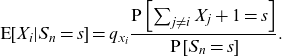
 \begin{align} \textrm{E}[X_i|S_n=s] & = \frac{ \textrm{E}[ X_i{\unicode[Times]{x1D7D9}}_{S_n=s}]}{\textrm{P}[S_n=s]} \nonumber\\[5pt] & = \frac{1}{ \textrm{P}[S_n=s] } \left( \int_{\mathbb{R}}\textrm{E}\left[x{\unicode[Times]{x1D7D9}}_{x+\sum_{j\ne i}X_j = s }\right]\, \textrm{d}\textrm{P}_{X_i}(x) \right) \nonumber \\[5pt] & = \frac{1}{ \textrm{P}[S_n=s] } \left( \int_{\mathbb{R}} x\cdot \textrm{P}\left[x+\sum_{j\ne i}X_j = s \right]\, \textrm{d}\textrm{P}_{X_i}(x) \right) \nonumber \\[5pt]& = \frac{ 1 } { \textrm{P}[S_n=s] } a_i\cdot \textrm{P}\left[ a_i +\sum_{j\ne i}X_j = s \right] \cdot q_{x_i}\,.\end{align}
Formula (2.2) provides the actuary with a practical way to compute conditional expectations
 $\textrm{E}[X_{i}|S_{n}=s]$
. Computation time nevertheless grows with the number n of participants. Henceforth, we assume that
$\textrm{E}[X_{i}|S_{n}=s]$
. Computation time nevertheless grows with the number n of participants. Henceforth, we assume that
 $a_i = a + k_i\cdot h$
,
$a_i = a + k_i\cdot h$
,
 $i=1,2,\ldots,n$
for
$i=1,2,\ldots,n$
for
 $k_i\in\mathbb{N}$
and
$k_i\in\mathbb{N}$
and
 $a,h\in\mathbb{R}^+$
.
$a,h\in\mathbb{R}^+$
.
2.3 Comonotonic mortality credits
2.3.1 Definition
A common property for a mortality risk sharing scheme is that the extra amount paid to participant i if he or she survives increases with the amount
 $S_{n}$
of mortality credits to be distributed at maturity. This property is referred to as the comonotonicity property and means for the conditional mean risk sharing rule that
$S_{n}$
of mortality credits to be distributed at maturity. This property is referred to as the comonotonicity property and means for the conditional mean risk sharing rule that
 \begin{equation}s\mapsto \textrm{E}[X_{i}|S_{n}=s]\text{ is nondecreasing over }\mathcal{S}_{n}\text{ for every }i\,. \end{equation}
If (2.3) holds true then mortality credits all move in the same direction with
 $S_n$
, increasing when
$S_n$
, increasing when
 $S_n$
increases and decreasing when
$S_n$
increases and decreasing when
 $S_n$
decreases, and the random vector
$S_n$
decreases, and the random vector
 $(\textrm{E}[X_1|S_{n}=s],\ldots,\textrm{E}[X_n|S_n])$
is said to be comonotonic. We refer the reader to Dhaene et al. (Reference Dhaene, Denuit, Goovaerts, Kaas and Vyncke2002a,b) for a general presentation of comonotonicity. It is important to stress that (2.3) is not in general valid (counterexamples are easy to build, as shown next), but some important cases for which the property holds have been studied in Denuit and Robert (Reference Denuit and Robert2021b).
$(\textrm{E}[X_1|S_{n}=s],\ldots,\textrm{E}[X_n|S_n])$
is said to be comonotonic. We refer the reader to Dhaene et al. (Reference Dhaene, Denuit, Goovaerts, Kaas and Vyncke2002a,b) for a general presentation of comonotonicity. It is important to stress that (2.3) is not in general valid (counterexamples are easy to build, as shown next), but some important cases for which the property holds have been studied in Denuit and Robert (Reference Denuit and Robert2021b).
2.3.2 Comonotonicity and heterogeneity in invested amounts
It is easy to see that the dispersion of the accumulated distributions
 $a_{1},a_{2},\ldots ,a_{n}$
plays a crucial role in that respect. To see why this is the case, assume that all
$a_{1},a_{2},\ldots ,a_{n}$
plays a crucial role in that respect. To see why this is the case, assume that all
 $a_{1},a_{2},\ldots ,a_{n}$
are different. If
$a_{1},a_{2},\ldots ,a_{n}$
are different. If
 $a_{i}$
cannot be written as a sum of some other
$a_{i}$
cannot be written as a sum of some other
 $a_{j}$
’s, then the event
$a_{j}$
’s, then the event
 $\{S_{n}=a_{i}\}$
is equivalent to the event
$\{S_{n}=a_{i}\}$
is equivalent to the event
 $\{I_{i}=0,I_{j}=1$
for
$\{I_{i}=0,I_{j}=1$
for
 $j\neq i\}$
and it follows that
$j\neq i\}$
and it follows that
 $\textrm{E}[X_{i}|S_{n}=a_{i}]=a_{i}$
. If all participants die, then we have
$\textrm{E}[X_{i}|S_{n}=a_{i}]=a_{i}$
. If all participants die, then we have
 \begin{equation*}\textrm{E}\left[X_{i}\,\Big|\,S_{n}=\sum_{j=1}^{n}a_{j}\right]=a_{i}\,.\end{equation*}
Therefore, for a finite pool size n and
 $a_{1},a_{2},\ldots ,a_{n}$
as described before, comonotonicity cannot hold unless conditional expectations are actually constant. Heterogeneity in invested amounts thus impacts on survivor funds. Sections 3 and 4 study the case where all contributed amounts
$a_{1},a_{2},\ldots ,a_{n}$
as described before, comonotonicity cannot hold unless conditional expectations are actually constant. Heterogeneity in invested amounts thus impacts on survivor funds. Sections 3 and 4 study the case where all contributed amounts
 $a_i$
are equal but participants are subject to different death probabilities, and the case where different contributions are allowed but selected from a predefined menu (limited heterogeneity). Before proceeding with this analysis, let us explain why comonotonic mortality credits ease the management of survivor funds by considering possible guarantees that may be offered to participants.
$a_i$
are equal but participants are subject to different death probabilities, and the case where different contributions are allowed but selected from a predefined menu (limited heterogeneity). Before proceeding with this analysis, let us explain why comonotonic mortality credits ease the management of survivor funds by considering possible guarantees that may be offered to participants.
2.3.3 Minimum guarantees
Participants to survivor funds are exposed to randomness in mortality credits. This is generally the case with tontine-like arrangements. The need for protection has been addressed in several papers and resulted for instance in hybrid schemes such as the tonuity proposed by Chen et al. (Reference Chen, Hieber and Klein2019) and the tontine with minimum guarantee in Chen and Rach (Reference Chen and Rach2019).
In order to ensure that participants get a minimum payoff, it seems to be desirable to reinsure the lower layer of
 $S_n$
: if
$S_n$
: if
 $S_n$
falls below a given threshold w then the (re-)insurer covers the shortfall
$S_n$
falls below a given threshold w then the (re-)insurer covers the shortfall
 $(w-S_n)_+ = \max\{w-S_n,\,0\}$
. A natural candidate for w consists in a given percentage of
$(w-S_n)_+ = \max\{w-S_n,\,0\}$
. A natural candidate for w consists in a given percentage of
 $\textrm{E}[S_n]=\sum_{i=1}^nq_{x_i}a_i$
. For instance, one could set
$\textrm{E}[S_n]=\sum_{i=1}^nq_{x_i}a_i$
. For instance, one could set
 $w=0.9\cdot \textrm{E}[S_n]$
if pool members are ready to accept mortality credits that are at most 10% below their expected value for the entire pool.
$w=0.9\cdot \textrm{E}[S_n]$
if pool members are ready to accept mortality credits that are at most 10% below their expected value for the entire pool.
When mortality credits are comonotonic, the global threshold w on the aggregate mortality credits
 $S_n$
to be shared among participants can easily be split into individual amounts
$S_n$
to be shared among participants can easily be split into individual amounts
 $w_i$
. Here,
$w_i$
. Here,
 $w_i$
is the minimal guarantee on the share of mortality credits allocated to participant i, as shown next. Under assumption (2.3), there exist
$w_i$
is the minimal guarantee on the share of mortality credits allocated to participant i, as shown next. Under assumption (2.3), there exist
 $w_1,\ldots,w_n$
such that
$w_1,\ldots,w_n$
such that
 $\sum_{i=1}^nw_i=w$
and the identities
$\sum_{i=1}^nw_i=w$
and the identities
 \begin{equation} (w-S_n)_+=\sum_{i=1}^n(w_i-\textrm{E}[X_i|S_n])_+\text{ and }(S_n-w)_+=\sum_{i=1}^n(\textrm{E}[X_i|S_n]-w_i)_+\end{equation}
both hold true. Formula (2.4) can be found in the proof of Theorem 6 in Kaas et al. (Reference Kaas, Dhaene, Vyncke, Goovaerts and Denuit2002); see the first formula on p. 78. The decomposition of
 $(w-S_n)_+$
appearing in (2.4) allows us to charge each participant with his or her own contribution to the (re-)insurance premium, based on the respective
$(w-S_n)_+$
appearing in (2.4) allows us to charge each participant with his or her own contribution to the (re-)insurance premium, based on the respective
 $(w_i-\textrm{E}[X_i|S_n])_+$
entering the decomposition of the lower layer
$(w_i-\textrm{E}[X_i|S_n])_+$
entering the decomposition of the lower layer
 $(w-S_n)_+$
. The price of the (re-)insurance treaty can thus be split according to (2.4), participant i paying
$(w-S_n)_+$
. The price of the (re-)insurance treaty can thus be split according to (2.4), participant i paying
 $(1+\theta)\textrm{E}[(w_i-\textrm{E}[X_i|S_n])_+]$
summing up to
$(1+\theta)\textrm{E}[(w_i-\textrm{E}[X_i|S_n])_+]$
summing up to
 $(1+\theta)\textrm{E}[(w-S_n)_+]$
where
$(1+\theta)\textrm{E}[(w-S_n)_+]$
where
 $\theta$
is the loading applied by the reinsurer. Although proportional loadings are common in practice, notably when expenses are referred to, a safety loading could rely on diversification arguments, then being based on some risk measure. The results of this section still apply in that case provided the selected risk measure is additive for comonotonic risks. All spectral risk measures enjoy this property, including Value-at-Risk or Tail-Value-at-Risk.
$\theta$
is the loading applied by the reinsurer. Although proportional loadings are common in practice, notably when expenses are referred to, a safety loading could rely on diversification arguments, then being based on some risk measure. The results of this section still apply in that case provided the selected risk measure is additive for comonotonic risks. All spectral risk measures enjoy this property, including Value-at-Risk or Tail-Value-at-Risk.
Identities (2.4) also provide the analyst with the right way to allocate
 $\max\{S_n,w\}$
among participants:
$\max\{S_n,w\}$
among participants:
 \begin{eqnarray}\max\{S_n,w\}&=&w+(S_n-w)_+ \notag \\[5pt]&=&\sum_{i=1}^n\left(w_i+(\textrm{E}[X_i|S_n]-w_i)_+\right) \notag \\[5pt]&=&\sum_{i=1}^n\max\{\textrm{E}[X_i|S_n],w_i\}. \end{eqnarray}
Then,
 $\max\{S_n,w\}$
is distributed among participants according to formula (2.5). Precisely, participant i gets mortality credits
$\max\{S_n,w\}$
is distributed among participants according to formula (2.5). Precisely, participant i gets mortality credits
 $\max\{\textrm{E}[X_i|S_n],w_i\}$
when the pool buys protection ensuring mortality credits
$\max\{\textrm{E}[X_i|S_n],w_i\}$
when the pool buys protection ensuring mortality credits
 $\max\{S_n,w\}$
.
$\max\{S_n,w\}$
.
3 Identical amounts of contribution
In this section, we consider the case where participants’ accumulated assets are identical across the pool, that is,
 $a_{i}=a$
for some
$a_{i}=a$
for some
 $a>0$
.
$a>0$
.
3.1 Risk elimination
We know from Denuit and Robert (Reference Denuit and Robert2021c) that the income
 $\textrm{E}[X_{i}|S_{n}]$
decreases in convex order with the size n of the pool. This ensures that the variance of
$\textrm{E}[X_{i}|S_{n}]$
decreases in convex order with the size n of the pool. This ensures that the variance of
 $\textrm{E}[X_{i}|S_{n}]$
is nonincreasing when n gets larger. In that respect, conditional mean risk sharing offers a way to distribute the total mortality credits
$\textrm{E}[X_{i}|S_{n}]$
is nonincreasing when n gets larger. In that respect, conditional mean risk sharing offers a way to distribute the total mortality credits
 $S_{n}$
among the n participants so that enlarging the pool is always beneficial and participants thus prefer joining the larger pool. It is therefore interesting to study mortality credits when n becomes large. The following result shows that diversification operates within survivor funds, under the conditional mean risk sharing rule.
$S_{n}$
among the n participants so that enlarging the pool is always beneficial and participants thus prefer joining the larger pool. It is therefore interesting to study mortality credits when n becomes large. The following result shows that diversification operates within survivor funds, under the conditional mean risk sharing rule.
Proposition 3.1. If
 $a_{i}=a$
for all i and the sequence of probabilities
$a_{i}=a$
for all i and the sequence of probabilities
 $q_{x_i}$
is contained in a closed subinterval of [0,1], then we have
$q_{x_i}$
is contained in a closed subinterval of [0,1], then we have
 \begin{equation*}\textrm{Var}\left[\textrm{E}[X_{i}|S_{n+1}]\right]\leq \textrm{Var}\left[\textrm{E}[X_{i}|S_{n}]\right]{\;for\;all\;}n\;{ and }\;\lim_{n\to\infty}\textrm{Var}\left[\textrm{E}[X_{i}|S_{n}]\right]=0\,.\end{equation*}
Proof. The inequality for the variance of mortality credits directly follows from a general result in Denuit and Robert (Reference Denuit and Robert2021c). Proposition 2.1 in that paper shows that
 $\textrm{E}[X_{i}|S_{n}]$
decreases in the convex order for any independent random variables
$\textrm{E}[X_{i}|S_{n}]$
decreases in the convex order for any independent random variables
 $X_i$
, which implies the announced ranking for variances. The mean-squared convergence of
$X_i$
, which implies the announced ranking for variances. The mean-squared convergence of
 $\textrm{E}[X_{i}|S_{n}]$
to
$\textrm{E}[X_{i}|S_{n}]$
to
 $\textrm{E}[X_{i}]$
can be deduced from Strasser (Reference Strasser2012) who derived large-pool approximations for
$\textrm{E}[X_{i}]$
can be deduced from Strasser (Reference Strasser2012) who derived large-pool approximations for
 $\textrm{E}[X_{i}|S_{n}]$
in the particular case when
$\textrm{E}[X_{i}|S_{n}]$
in the particular case when
 $a_{i}=1$
for all i. In Theorem 2.1 of this paper, it is indeed proved that
$a_{i}=1$
for all i. In Theorem 2.1 of this paper, it is indeed proved that
 \begin{equation*}\textrm{E}[X_{i}|S_{n}]=q_{x_{i}}+\frac{q_{x_{i}}(1-q_{x_{i}})}{\sqrt{\textrm{Var}[S_{n}]}}Z_{n}+\frac{\tau _{i,n}}{\textrm{Var}[S_{n}]}{(Z_{n}^{2}-1)}+r_{ni}\left( Z_{n}\right)\end{equation*}
where
 \begin{equation*}Z_{n}=\frac{S_{n}-\textrm{E}[S_{n}]}{\sqrt{\textrm{Var}[S_{n}]}},\qquad \tau_{i,n}=q_{x_{i}}(1-q_{x_{i}})\left(q_{x_{i}}-\frac{1}{\textrm{Var}[S_{n}]}\sum_{j=1}^{n}q_{x_{j}}^{2}(1-q_{x_{j}})\right),\end{equation*}
and
 $\textrm{E}[|r_{ni}\left( Z_{n}\right) |]=O\left( n^{-3/2}\right) $
. Using Corollary 5.2 and Lemma 5.3 of the same paper, it is also true that
$\textrm{E}[|r_{ni}\left( Z_{n}\right) |]=O\left( n^{-3/2}\right) $
. Using Corollary 5.2 and Lemma 5.3 of the same paper, it is also true that
 $\textrm{E}[|r_{ni}\left( Z_{n}\right) |^{2}]=O\left( n^{-3/2}\right) $
. Since
$\textrm{E}[|r_{ni}\left( Z_{n}\right) |^{2}]=O\left( n^{-3/2}\right) $
. Since
 \begin{align*}\left( \textrm{E}[X_{i}|S_{n}]-q_{x_{i}}\right) ^{2} & \leq 4\left( \frac{q_{x_{i}}(1-q_{x_{i}})}{\sqrt{\textrm{Var}[S_{n}]}}Z_{n}\right) ^{2}+4\left(\frac{\tau _{i,n}}{\textrm{Var}[S_{n}]}{(Z_{n}^{2}-1)}\right) ^{2}\\[5pt] & +4\left(r_{ni}\left( Z_{n}\right) \right) ^{2},\end{align*}
we deduce that the variance of
 $\textrm{E}[X_{i}|S_{n}]$
tends to 0 as
$\textrm{E}[X_{i}|S_{n}]$
tends to 0 as
 $n\rightarrow \infty $
. This ends the proof.
$n\rightarrow \infty $
. This ends the proof.
The limit in Proposition 3.1 extends the classical weak law of large numbers for averages of independent and identically distributed
 $X_i$
corresponding to mortality credits allocations within homogeneous pools as shown in (2.1). Proposition 3.1 shows that individual risk can generally be fully eliminated in an infinitely large pool.
$X_i$
corresponding to mortality credits allocations within homogeneous pools as shown in (2.1). Proposition 3.1 shows that individual risk can generally be fully eliminated in an infinitely large pool.
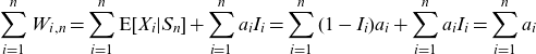
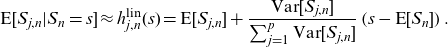
The following numerical example illustrates the results derived in Proposition 3.1. All calculations are carried out with the distr package available in R, see distr.r-forge.r-project.org/.
Example 3.2. Consider n participants partitioned into two groups: 60% of them are subject to a death probability equal to 0.1 and the remaining 40% of them to a death probability equal to 0.2. All values
 $a_i$
are set to 1. The left panel in Figure 1 shows the variance of
$a_i$
are set to 1. The left panel in Figure 1 shows the variance of
 $\textrm{E}[X_i|S_n]/a_i$
for
$\textrm{E}[X_i|S_n]/a_i$
for
 $n\in\{10,20,30,\ldots,1000\}$
. The decreasing trend to 0 established in Proposition 3.1 is clearly visible there. The lower quartile, the median and the upper quartile (that is, quantiles associated to probability levels 0.25, 0.5 and 0.75) of
$n\in\{10,20,30,\ldots,1000\}$
. The decreasing trend to 0 established in Proposition 3.1 is clearly visible there. The lower quartile, the median and the upper quartile (that is, quantiles associated to probability levels 0.25, 0.5 and 0.75) of
 $\textrm{E}[X_i|S_n]/a_i$
are displayed in the other two panels of Figure 1 for
$\textrm{E}[X_i|S_n]/a_i$
are displayed in the other two panels of Figure 1 for
 $n\in\{100,200,300,\ldots,1000\}$
for a participant in group 1 in the middle panel and for a participant in group 2 in the right panel. We can see there that the interquartile range narrows at speed
$n\in\{100,200,300,\ldots,1000\}$
for a participant in group 1 in the middle panel and for a participant in group 2 in the right panel. We can see there that the interquartile range narrows at speed
 $n^{-1/2}$
.
$n^{-1/2}$
.
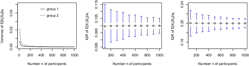
Figure 1. Variance of
 $\textrm{E}[X_i|S_n]/a_i$
as a function of
$\textrm{E}[X_i|S_n]/a_i$
as a function of
 $n\in\{10,20,30,\ldots,1000\}$
(left panel) for a participant in group 1 (continuous line) and in group 2 (broken line), median and interquartile range (IQR) of
$n\in\{10,20,30,\ldots,1000\}$
(left panel) for a participant in group 1 (continuous line) and in group 2 (broken line), median and interquartile range (IQR) of
 $\textrm{E}[X_i|S_n]/a_i$
for
$\textrm{E}[X_i|S_n]/a_i$
for
 $n\in\{100,200,300,\ldots,1000\}$
in group 1 (middle panel) and in group 2 (right panel) for the pool described in Example 3.2. Horizontal lines in the central and right panels correspond to expected mortality credits.
$n\in\{100,200,300,\ldots,1000\}$
in group 1 (middle panel) and in group 2 (right panel) for the pool described in Example 3.2. Horizontal lines in the central and right panels correspond to expected mortality credits.
3.2 Comonotonic mortality credits
If all the contributions are equal, then the comonotonicity property (2.3) always holds true, as formally shown next.
Proposition 3.3. If
 $a_{i}=a$
for all i, then the comonotonicity property (2.3) holds true over
$a_{i}=a$
for all i, then the comonotonicity property (2.3) holds true over
 $\mathcal{S}_{n}=\{0,a,2a,\ldots ,na\}$
.
$\mathcal{S}_{n}=\{0,a,2a,\ldots ,na\}$
.
Proof. We can assume without loss of generality that
 $a=1$
. Considering (2.2) with
$a=1$
. Considering (2.2) with
 $a_i=1$
for all i, we can see that
$a_i=1$
for all i, we can see that
 \begin{equation*}\textrm{E}[X_{i}|S_{n}=s] =q_{x_{i}}\frac{\textrm{P}\left[ \sum_{j\neq i}X_{j}+1=s\right]} {\textrm{P}\left[ S_n=s\right]}.\end{equation*}
Hence, comonotonicity holds provided the ratio of probabilities appearing in the latter expression is nondecreasing. This means that
 $S_n$
is smaller than
$S_n$
is smaller than
 $\sum_{j\neq i}X_j+1$
in the sense of the likelihood ratio order. The announced result then follows from stochastic inequality (1.5) in Xu and Balakrishnan (Reference Xu and Balakrishnan2011). Precisely, these authors established that given two sets of independent Bernoulli random variables
$\sum_{j\neq i}X_j+1$
in the sense of the likelihood ratio order. The announced result then follows from stochastic inequality (1.5) in Xu and Balakrishnan (Reference Xu and Balakrishnan2011). Precisely, these authors established that given two sets of independent Bernoulli random variables
 $\{J_1,J_2,\ldots,J_n\}$
and
$\{J_1,J_2,\ldots,J_n\}$
and
 $\{K_1,K_2,\ldots,K_n\}$
with respective means
$\{K_1,K_2,\ldots,K_n\}$
with respective means
 $q_{J,1},q_{J,2},\ldots,q_{J,n}$
and
$q_{J,1},q_{J,2},\ldots,q_{J,n}$
and
 $q_{K,1},q_{K,2},\ldots,q_{K,n}$
such that
$q_{K,1},q_{K,2},\ldots,q_{K,n}$
such that
 $q_{J,1}\leq q_{J,2}\leq\ldots\leq q_{J,n}$
and
$q_{J,1}\leq q_{J,2}\leq\ldots\leq q_{J,n}$
and
 $q_{K,1}\leq q_{K,2}\leq \ldots \leq q_{K,n}$
,
$q_{K,1}\leq q_{K,2}\leq \ldots \leq q_{K,n}$
,
 \begin{equation*}\sum_{l=1}^m\frac{1}{q_{J,l}}\leq \sum_{l=1}^m\frac{1}{q_{K,l}}\text{ for }m=1,\ldots,n\Rightarrow s\mapsto\frac{\textrm{P}\left[\sum_{l=1}^nJ_l=s\right]}{\textrm{P}\left[\sum_{l=1}^nK_l=s\right]} \text{ is nondecreasing}.\end{equation*}
It suffices to apply this result here with
 $q_{J,l}=q_{K,l}=q_{x_l}$
for
$q_{J,l}=q_{K,l}=q_{x_l}$
for
 $l\neq i $
,
$l\neq i $
,
 $q_{J,i}=1$
and
$q_{J,i}=1$
and
 $q_{K,i}=q_{x_i}$
(with appropriate re-indexing). This ends the proof.
$q_{K,i}=q_{x_i}$
(with appropriate re-indexing). This ends the proof.
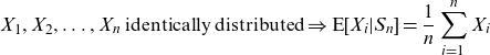
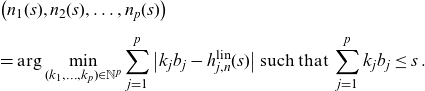
The following numerical example illustrates the comonotonicity property established in Proposition 3.3.
Example 3.4. Let us consider the same pool as in Example 3.2 with participants partitioned into two groups: 60% of them are subject to a death probability equal to 0.1 and the remaining 40% of them to a death probability equal to 0.2, with
 $a_i=1$
for all i. The functions
$a_i=1$
for all i. The functions
 $s\mapsto\textrm{E}[X_i|S_n=s]$
are displayed in Figure 2 for
$s\mapsto\textrm{E}[X_i|S_n=s]$
are displayed in Figure 2 for
 $n\in\{10,100\}$
for a participant in group 1 or in group 2. The increasingness established in Proposition 3.3 is clearly visible there.
$n\in\{10,100\}$
for a participant in group 1 or in group 2. The increasingness established in Proposition 3.3 is clearly visible there.
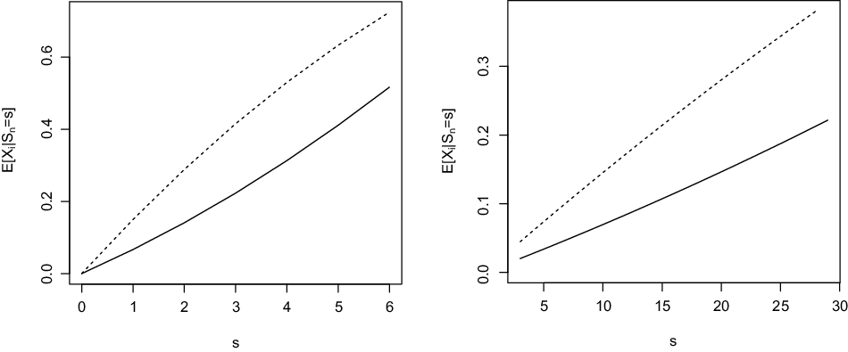
Figure 2. Functions
 $s\mapsto\textrm{E}[X_i|S_n=s]$
for
$s\mapsto\textrm{E}[X_i|S_n=s]$
for
 $n=10$
(left panel) and
$n=10$
(left panel) and
 $n=100$
(right panel) for a participant in group 1 (continuous line) and in group 2 (broken line) in the pool described in Example 3.2.
$n=100$
(right panel) for a participant in group 1 (continuous line) and in group 2 (broken line) in the pool described in Example 3.2.
4 Varying amounts of contribution
4.1 Risk elimination
When contributions vary among participants, some structure must be imposed on
 $a_1,\ldots,a_n$
to get diversification within the survivor fund, as shown by the following example which appears to be similar to developments in Section 2.3.2.
$a_1,\ldots,a_n$
to get diversification within the survivor fund, as shown by the following example which appears to be similar to developments in Section 2.3.2.
Example 4.1. Let
 $a_i$
be even integers except for the odd integer
$a_i$
be even integers except for the odd integer
 $a_1$
. Then,
$a_1$
. Then,
 $X_1=a_1$
when
$X_1=a_1$
when
 $S_n$
is odd and
$S_n$
is odd and
 $X_1=0$
when
$X_1=0$
when
 $S_n$
is even so that
$S_n$
is even so that
 $\textrm{E}[X_1|S_n]=X_1$
and no diversification operates for participant 1.
$\textrm{E}[X_1|S_n]=X_1$
and no diversification operates for participant 1.
The difference between the present paper and the previous works devoted to conditional mean risk sharing rule appears to be the knowledge of amounts that could be lost and can identify the participant who died in some extreme cases. To solve this issue, we assume in this section that only a limited choice is offered to participants for the amounts of contribution. Precisely, we assume that participants choose their level of contributions within a predefined menu
 $b_j = a + k_j \cdot h$
, for
$b_j = a + k_j \cdot h$
, for
 $j=1,2,\ldots,p$
, for consecutive
$j=1,2,\ldots,p$
, for consecutive
 $k_j\in\mathbb{N}$
and
$k_j\in\mathbb{N}$
and
 $p\in\mathbb{N}$
. The number of possible contributions p in this predefined menu
$p\in\mathbb{N}$
. The number of possible contributions p in this predefined menu
 $\{b_{1},\ldots,b_p\}$
does not vary with n. Theoretical results are valid for any p but diversification is better and the proposed approximations are more accurate when p is smaller. The predefined menu still contains Example 4.1 as special case. However, participant 1 is now part of a pool of others with the same accumulated distribution
$\{b_{1},\ldots,b_p\}$
does not vary with n. Theoretical results are valid for any p but diversification is better and the proposed approximations are more accurate when p is smaller. The predefined menu still contains Example 4.1 as special case. However, participant 1 is now part of a pool of others with the same accumulated distribution
 $a_1$
.
$a_1$
.
Let
 $\mathcal{G}_{j}=\{i|a_{i}=b_{j}\}$
be the group of participants with accumulated contribution equal to
$\mathcal{G}_{j}=\{i|a_{i}=b_{j}\}$
be the group of participants with accumulated contribution equal to
 $b_{j}$
,
$b_{j}$
,
 $j=1,2,\ldots,p$
. Then,
$j=1,2,\ldots,p$
. Then,
 \begin{equation}S_{j,n}=\sum_{i\in \mathcal{G}_{j}}X_{i}=b_{j}\sum_{i\in \mathcal{G}_{j}}\left( 1-I_{i}\right)\end{equation}
is the total amount of mortality credits generated by group
 $\mathcal{G}_{j}$
. Henceforth, we denote as
$\mathcal{G}_{j}$
. Henceforth, we denote as
 $n_j=\#\mathcal{G}_{j}$
the number of participants in group j, with accumulated contribution
$n_j=\#\mathcal{G}_{j}$
the number of participants in group j, with accumulated contribution
 $a_i=b_j$
.
$a_i=b_j$
.
We are now in a position to assess diversification effects within survivor funds, under conditional mean risk sharing rule when contributions are selected from a predefined menu (limited heterogeneity) by keeping p fixed when n increases. In this way, we can show that full risk elimination is still possible provided all group sizes
 $n_j$
tend to infinity. This is precisely stated next.
$n_j$
tend to infinity. This is precisely stated next.
Proposition 4.2. Let p be a fixed integer and the sequence of probabilities
 $q_{x_i}$
is contained in a closed subinterval of [0,1]. If
$q_{x_i}$
is contained in a closed subinterval of [0,1]. If
 $a_{i}\in \{b_{1},\ldots,b_p\}$
for all i, then we have
$a_{i}\in \{b_{1},\ldots,b_p\}$
for all i, then we have
 \begin{equation*}\textrm{Var}\left[\textrm{E}[X_{i}|S_{n+1}]\right]\leq \textrm{Var}\left[\textrm{E}[X_{i}|S_{n}]\right]\;{ for\;all\;}n\;{ and }\;\lim_{n_1,n_2,\ldots,n_p\to\infty}\textrm{Var}\left[\textrm{E}[X_{i}|S_{n}]\right]=0.\end{equation*}
Proof. The inequality for the variance of mortality credits again follows from Denuit and Robert (Reference Denuit and Robert2021c). The mean-squared convergence of
 $\textrm{E}[X_{i}|S_{n}]$
to
$\textrm{E}[X_{i}|S_{n}]$
to
 $\textrm{E}[X_{i}]$
can be deduced from the following property established by Denuit and Robert (Reference Denuit and Robert2021f): for any independent random variables U, V and W,
$\textrm{E}[X_{i}]$
can be deduced from the following property established by Denuit and Robert (Reference Denuit and Robert2021f): for any independent random variables U, V and W,
 $\textrm{E}[U|U+V+W]$
is smaller or equal than
$\textrm{E}[U|U+V+W]$
is smaller or equal than
 $\textrm{E}[U|U+V]$
in the sense of the convex order so that
$\textrm{E}[U|U+V]$
in the sense of the convex order so that
 \begin{equation*}\textrm{Var}\left[\textrm{E}[U|U+V+W]\right]\leq \textrm{Var}\left[\textrm{E}[U|U+V]\right].\end{equation*}
Without the loss of generality, we can set
 $i=1$
and assume that
$i=1$
and assume that
 $a_1=b_1$
. Applying this result to
$a_1=b_1$
. Applying this result to
 $U=X_1$
,
$U=X_1$
,
 $V=S_{1,n}$
and
$V=S_{1,n}$
and
 $W=\sum_{j=2}^pS_{j,n}$
shows that
$W=\sum_{j=2}^pS_{j,n}$
shows that
 \begin{equation*} \textrm{Var}\left[\textrm{E}[X_1|S_{n}]\right]\leq \textrm{Var}\left[\textrm{E}[X_1|S_{1,n}]\right].\end{equation*}
Since the variance appearing on the right-hand side tends to 0 when
 $n_1$
tends to infinity by Proposition 3.1, this ends the proof.
$n_1$
tends to infinity by Proposition 3.1, this ends the proof.
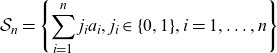
Example 4.3 illustrates the convergence established in Proposition 4.2.
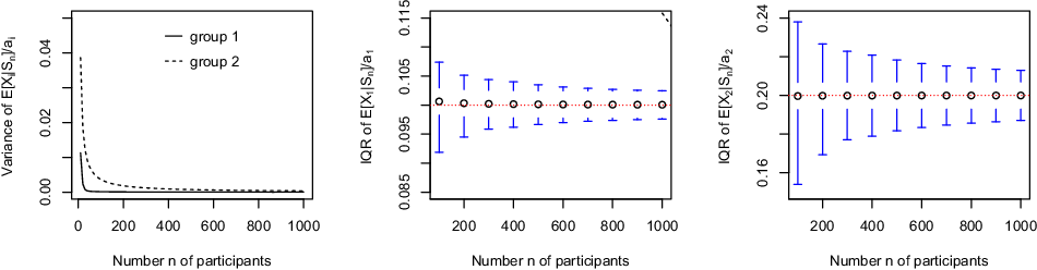
Figure 3. Variance of
 $\textrm{E}[X_i|S_n]/a_i$
as a function of
$\textrm{E}[X_i|S_n]/a_i$
as a function of
 $n\in\{10,20,30,\ldots,1000\}$
(left panel) for a participant in group 1 (continuous line) and in group 2 (broken line), median and interquartile range (IQR) of
$n\in\{10,20,30,\ldots,1000\}$
(left panel) for a participant in group 1 (continuous line) and in group 2 (broken line), median and interquartile range (IQR) of
 $\textrm{E}[X_i|S_n]/a_i$
for
$\textrm{E}[X_i|S_n]/a_i$
for
 $n\in\{100,200,300,\ldots,1000\}$
in group 1 (middle panel) and in group 2 (right panel) for the pool described in Example 4.3. Horizontal lines in the central and right panels correspond to expected mortality credits.
$n\in\{100,200,300,\ldots,1000\}$
in group 1 (middle panel) and in group 2 (right panel) for the pool described in Example 4.3. Horizontal lines in the central and right panels correspond to expected mortality credits.
Example 4.3. Consider the pool described in Example 3.2 but assume now that
 $a_i=1$
for the participants subject to death probability 0.1 (60% of the pool) and
$a_i=1$
for the participants subject to death probability 0.1 (60% of the pool) and
 $a_i=3$
for the participants subject to death probability 0.2. Figure 3 shows the variance of
$a_i=3$
for the participants subject to death probability 0.2. Figure 3 shows the variance of
 $\textrm{E}[X_i|S_n]/a_i$
for
$\textrm{E}[X_i|S_n]/a_i$
for
 $n\in\{10,20,30,\ldots,1000\}$
. The decreasing trend to 0 established in Proposition 4.2 is clearly visible there. The lower quartile, the median and the upper quartile (that is, quantiles associated to probability levels 0.25, 0.5 and 0.75) of
$n\in\{10,20,30,\ldots,1000\}$
. The decreasing trend to 0 established in Proposition 4.2 is clearly visible there. The lower quartile, the median and the upper quartile (that is, quantiles associated to probability levels 0.25, 0.5 and 0.75) of
 $\textrm{E}[X_i|S_n]/a_i$
are displayed in the other two panels of Figure 2 for
$\textrm{E}[X_i|S_n]/a_i$
are displayed in the other two panels of Figure 2 for
 $n\in\{100,200,300,\ldots,1000\}$
for a participant in group 1 in the middle panel and for a participant in group 2 in the right panel. We can see there that the interquartile range narrows at speed
$n\in\{100,200,300,\ldots,1000\}$
for a participant in group 1 in the middle panel and for a participant in group 2 in the right panel. We can see there that the interquartile range narrows at speed
 $n^{-1/2}$
. Compared to Example 3.2, we can see here that the mean and medians differ in smaller pools while the medians converge to the mean within larger pools.
$n^{-1/2}$
. Compared to Example 3.2, we can see here that the mean and medians differ in smaller pools while the medians converge to the mean within larger pools.
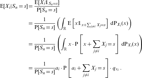
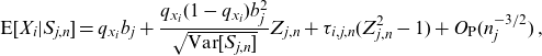
Figure 4 compares the variance of the case where groups 1 and 2 are pooled together (continuous line) as a function of the pool size n to the case where group 1 (pool size
 $40\%\cdot n$
) and group 2 (pool size
$40\%\cdot n$
) and group 2 (pool size
 $60\%\cdot n$
) are treated separately. We observe that pooling the two heterogeneous groups reduces the variance and is beneficial for both groups.
$60\%\cdot n$
) are treated separately. We observe that pooling the two heterogeneous groups reduces the variance and is beneficial for both groups.
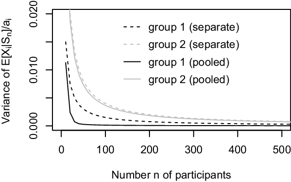
Figure 4. Variance of
 $\textrm{E}[X_i|S_n]/a_i$
as a function of
$\textrm{E}[X_i|S_n]/a_i$
as a function of
 $n\in\{10,20,30,\ldots,500\}$
for a participant in group 1 (black) and in group 2 (grey). We compare the case where the two groups are treated separately (broken line) to the case where both groups are pooled together (continuous line).
$n\in\{10,20,30,\ldots,500\}$
for a participant in group 1 (black) and in group 2 (grey). We compare the case where the two groups are treated separately (broken line) to the case where both groups are pooled together (continuous line).
4.2 Comonotonicity
In the general case of heterogeneous
 $a_i$
, comonotonicity property (2.3) does not necessarily hold as shown by the following example.
$a_i$
, comonotonicity property (2.3) does not necessarily hold as shown by the following example.
Example 4.4. Consider again the pool described in Example 4.3. The functions
 $s\mapsto\textrm{E}[X_i|S_n=s]$
are displayed in Figure 5 for
$s\mapsto\textrm{E}[X_i|S_n=s]$
are displayed in Figure 5 for
 $n\in\{10,20,50,100\}$
for a participant in group 1 or in group 2. We can see there that (2.3) does not hold for every i when n is small. Interestingly, when the size of the pool increases while keeping the same structure, the functions
$n\in\{10,20,50,100\}$
for a participant in group 1 or in group 2. We can see there that (2.3) does not hold for every i when n is small. Interestingly, when the size of the pool increases while keeping the same structure, the functions
 $s\mapsto \textrm{E}[X_{i}|S_{n}=s] $
ultimately become monotonic.
$s\mapsto \textrm{E}[X_{i}|S_{n}=s] $
ultimately become monotonic.
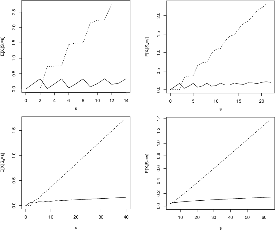
Figure 5. Functions
 $s\mapsto\textrm{E}[X_i|S_n=s]$
for
$s\mapsto\textrm{E}[X_i|S_n=s]$
for
 $n=10$
(upper left panel),
$n=10$
(upper left panel),
 $n=20$
(upper right panel),
$n=20$
(upper right panel),
 $n=50$
(lower left panel), and
$n=50$
(lower left panel), and
 $n=100$
(lower right panel), for a participant in group 1 (continuous line) and in group 2 (broken line) in the pool described in Example 7.
$n=100$
(lower right panel), for a participant in group 1 (continuous line) and in group 2 (broken line) in the pool described in Example 7.
The next section derives accurate approximations for mortality credits within large pools.
4.3 Large-pool comonotonic approximations to mortality credits
Within the groups
 $\mathcal{G}_{j}$
, we can apply the results of Section 3 since
$\mathcal{G}_{j}$
, we can apply the results of Section 3 since
 $a_{i}=b_{j}$
for all i. The idea is thus to distribute the mortality credits among the different groups
$a_{i}=b_{j}$
for all i. The idea is thus to distribute the mortality credits among the different groups
 $\mathcal{G}_{j}$
and then within each group. The amount
$\mathcal{G}_{j}$
and then within each group. The amount
 $S_{j,n}$
of mortality credits generated by
$S_{j,n}$
of mortality credits generated by
 $\mathcal{G}_{j}$
has been defined in (4.1). The first two moments of this random variable are given by
$\mathcal{G}_{j}$
has been defined in (4.1). The first two moments of this random variable are given by
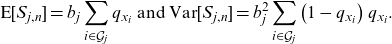 \begin{equation}\textrm{E}[S_{j,n}]=b_{j}\sum_{i\in \mathcal{G}_{j}}q_{x_{i}}\text{ and }\textrm{Var}[S_{j,n}]=b_{j}^{2}\sum_{i\in \mathcal{G}_{j}}\left( 1-q_{x_{i}}\right)q_{x_{i}}.\end{equation}
The total amount of mortality credits to be distributed among the n participants can be decomposed into
 $S_{n}=\sum_{j=1}^{p}S_{j,n}$
.
$S_{n}=\sum_{j=1}^{p}S_{j,n}$
.
We propose a hierarchical mortality credit sharing to distribute
 $S_{n}$
that proceeds in two steps. First, the total amount of mortality credits is shared between the groups
$S_{n}$
that proceeds in two steps. First, the total amount of mortality credits is shared between the groups
 $\mathcal{G}_1,\mathcal{G}_2,\ldots,\mathcal{G}_p$
with the help of the linear regression sharing rule
$\mathcal{G}_1,\mathcal{G}_2,\ldots,\mathcal{G}_p$
with the help of the linear regression sharing rule
 $h_{j,n}^{\textrm{lin}}$
. The latter only uses the two first moments of
$h_{j,n}^{\textrm{lin}}$
. The latter only uses the two first moments of
 $S_{j,n}$
and attributes to group
$S_{j,n}$
and attributes to group
 $\mathcal{G}_{j}$
the amount of mortality credits
$\mathcal{G}_{j}$
the amount of mortality credits
 \begin{equation*}\textrm{E}[S_{j,n}|S_{n}=s]\approx h_{j,n}^{\textrm{lin}}(s)=\textrm{E}[S_{j,n}]+\frac{\textrm{Var}[S_{j,n}]}{\sum_{j=1}^p\textrm{Var}[S_{j,n}]}\left( s-\textrm{E}[S_{n}]\right) .\end{equation*}
This approximation can be justified by the fact it is asymptotically equivalent to the conditional mean risk sharing rule as n and the numbers
 $n_{j}$
of participants in groups
$n_{j}$
of participants in groups
 $\mathcal{G}_{j}$
are large. In such a case, the amounts
$\mathcal{G}_{j}$
are large. In such a case, the amounts
 $S_{j,n}$
are approximately normally distributed with expected values
$S_{j,n}$
are approximately normally distributed with expected values
 $\textrm{E}[S_{j,n}]$
and variance
$\textrm{E}[S_{j,n}]$
and variance
 $\textrm{Var}[S_{j,n}]$
given in (4.2). The proposed approximation
$\textrm{Var}[S_{j,n}]$
given in (4.2). The proposed approximation
 $h_{j,n}^{\textrm{lin}}(s)$
corresponds to the conditional expectation of
$h_{j,n}^{\textrm{lin}}(s)$
corresponds to the conditional expectation of
 $S_{j,n}$
given
$S_{j,n}$
given
 $S_{n}=s$
in that limiting case. Notice that the functions
$S_{n}=s$
in that limiting case. Notice that the functions
 $s\mapsto h_{j,n}^{\textrm{lin}}(s)$
are also increasing in s so that the allocation of mortality credits between groups results in comonotonic shares.
$s\mapsto h_{j,n}^{\textrm{lin}}(s)$
are also increasing in s so that the allocation of mortality credits between groups results in comonotonic shares.
For
 $s\in \mathcal{S}_{n}$
, let us define the vector
$s\in \mathcal{S}_{n}$
, let us define the vector
 $\left(n_1(s),n_2(s),\ldots,n_p(s) \right)\in\mathbb{N}^p$
as
$\left(n_1(s),n_2(s),\ldots,n_p(s) \right)\in\mathbb{N}^p$
as
 \begin{align*}&\left(n_1( s),n_2 ( s),\ldots,n_p( s) \right)\\[5pt] &=\arg\min_{(k_1,\ldots,k_p)\in\mathbb{N}^p}\sum_{j=1}^p\big\vert k_{j}b_{j}-h_{j,n}^{\textrm{lin}}(s)\big\vert \text{ such that }\sum_{j=1}^pk_{j}b_{j}\le s\,.\end{align*}
For a realization s of
 $S_n$
,
$S_n$
,
 $n_{j}(s) $
provides a number of participants such that
$n_{j}(s) $
provides a number of participants such that
 $n_{j}(s)\cdot b_{j}$
is very close to the mortality credits
$n_{j}(s)\cdot b_{j}$
is very close to the mortality credits
 $h_{j,n}^{\textrm{lin}}(s)$
allocated to group j. This allocation cannot distribute more than the realized mortality credits, that is it needs to satisfy the budget constraint
$h_{j,n}^{\textrm{lin}}(s)$
allocated to group j. This allocation cannot distribute more than the realized mortality credits, that is it needs to satisfy the budget constraint
 $\sum_{j=1}^pk_{j}b_{j}\le s$
. Notice that the functions
$\sum_{j=1}^pk_{j}b_{j}\le s$
. Notice that the functions
 $s\mapsto n_{j}( s) $
are nondecreasing in s. The mortality credits allocated to participant i in group j are then defined as
$s\mapsto n_{j}( s) $
are nondecreasing in s. The mortality credits allocated to participant i in group j are then defined as
 $\textrm{E}\left[ X_{i}\,|\, S_{j,n}=n_{j}( S_{n})\cdot b_{j}\right]$
. This procedure is in fact similar to the approach developed in Denuit and Robert (Reference Denuit and Robert2021e) when pools are partitioned into teams and we end up with a comonotonic mortality credit allocation.
$\textrm{E}\left[ X_{i}\,|\, S_{j,n}=n_{j}( S_{n})\cdot b_{j}\right]$
. This procedure is in fact similar to the approach developed in Denuit and Robert (Reference Denuit and Robert2021e) when pools are partitioned into teams and we end up with a comonotonic mortality credit allocation.
The conditional expectation involved in the second step can be computed directly or the following approximation can be applied. Using Theorem 2.1 in Strasser (Reference Strasser2012), we obtainFootnote 1
 \begin{equation*}\textrm{E}[X_{i}|S_{j,n}]=q_{x_{i}}b_{j}+\frac{q_{x_{i}}(1-q_{x_{i}})b_{j}^{2}}{\sqrt{\textrm{Var}[S_{j,n}]}}Z_{j,n}+\tau_{i,j,n}{(Z_{j,n}^{2}-1)}+O_{\textrm{P}}(n_{j}^{-3/2})\,,\end{equation*}
where
 \begin{eqnarray*}Z_{j,n}&=&\frac{S_{j,n}-\textrm{E}[S_{j,n}]}{\sqrt{\textrm{Var}[S_{j,n}]}}\,,\\[5pt]\tau _{i,j,n}&=&{\frac{q_{x_{i}}(1-q_{x_{i}})b_{j}^{3}}{\textrm{Var}[S_{j,n}]}}\left(q_{x_{i}}-\frac{b_{j}^{2}}{\textrm{Var}[S_{j,n}]}\sum_{l\in \mathcal{G}_{j}}q_{x_{l}}^{2}(1-q_{x_{l}})\right)\,.\end{eqnarray*}
Letting
 \begin{equation*}H_{j,n}:=\frac{h_{j,n}^{\textrm{lin}}(S_{n})-\textrm{E}[S_{j,n}]}{\sqrt{\textrm{Var}[S_{j,n}]}}=\frac{\sqrt{\textrm{Var}[S_{j,n}]}}{\sum_{j=1}^p\textrm{Var}[S_{j,n}]}\left( S_{n}-\textrm{E}[S_{n}]\right)\,,\end{equation*}
we finally obtain that
 \begin{eqnarray*}&&\textrm{E}\left[ X_{i}|S_{j,n}=n_{j}( S_{n})\cdot b_{j}\right] \\[5pt]&=&q_{x_{i}}b_{j}+\frac{q_{x_{i}}(1-q_{x_{i}})b_{j}^{2}}{\sqrt{\textrm{Var}[S_{j,n}]}}H_{j,n}+\tau _{i,j,n}{(H_{j,n}^{2}-1)}+O_{\textrm{P}}(n_{j}^{-3/2}) \\[5pt]&=&q_{x_{i}}b_{j}+\frac{q_{x_{i}}(1-q_{x_{i}})b_{j}^{2}}{\sum_{i=1}^{n}q_{x_{i}}(1-q_{x_{i}})a_{i}^{2}}\left( S_{n}-\textrm{E}[S_{n}]\right) \\[5pt]&&+q_{x_{i}}(1-q_{x_{i}})b_{j}^{3}\left(q_{x_{i}}-\frac{b_{j}^{2}}{\textrm{Var}[S_{j,n}]}\sum_{l\in \mathcal{G}_{j}}q_{x_{l}}^{2}(1-q_{x_{l}})\right)\, \\[5pt] &&\times \left(\left( \frac{S_{n}-\textrm{E}[S_{n}]}{\sum_{i=1}^{n}q_{x_{i}}(1-q_{x_{i}})a_{i}^{2}}\right) ^{2}-\frac{1}{\textrm{Var}[S_{j,n}]}\right) \\[5pt]&&+O_{\textrm{P}}(n_{j}^{-3/2}).\end{eqnarray*}
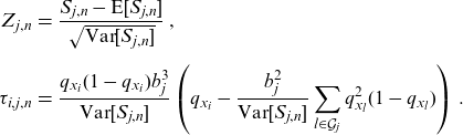
Example 4.5 illustrates the accuracy of the proposed approximation.
Example 4.5. Consider the pool described in Example 4.3 consisting of two groups: group 1 (60% of the pool) with
 $a_i=1$
and death probability 0.1 and group 2 (40% of the pool) with
$a_i=1$
and death probability 0.1 and group 2 (40% of the pool) with
 $a_i=3$
and death probability 0.2. Figure 6 shows the functions
$a_i=3$
and death probability 0.2. Figure 6 shows the functions
 $s\mapsto\textrm{E}[X_i|S_n=s]$
for
$s\mapsto\textrm{E}[X_i|S_n=s]$
for
 $n\in\{100,500,1000\}$
together with their large-pool approximations. For
$n\in\{100,500,1000\}$
together with their large-pool approximations. For
 $n=100$
, we can see there that the approximation is accurate in the central region but deteriorates in the tail. For larger pool sizes, the quality of the approximation seems to be excellent in this example.
$n=100$
, we can see there that the approximation is accurate in the central region but deteriorates in the tail. For larger pool sizes, the quality of the approximation seems to be excellent in this example.
Figure 6. Functions
 $s\mapsto\textrm{E}[X_i|S_n=s]$
(continuous line) and their large-pool approximation (broken line) for
$s\mapsto\textrm{E}[X_i|S_n=s]$
(continuous line) and their large-pool approximation (broken line) for
 $n=100$
(left panels),
$n=100$
(left panels),
 $n=500$
(middle panels), and
$n=500$
(middle panels), and
 $n=1000$
(right panels), and a participant in group 1 (upper panels) and in group 2 (lower panels) for the pool described in Example 4.3.
$n=1000$
(right panels), and a participant in group 1 (upper panels) and in group 2 (lower panels) for the pool described in Example 4.3.
5 Discussion
This paper studies large survivor funds where the number of participants tends to infinity, and the conditional mean risk sharing rule is adopted for the distribution of mortality credits. It has been shown that individual risk can be fully diversified within an infinitely large community, whatever the heterogeneity in mortality provided the amounts of contribution are selected from a predefined menu and pool sizes approach
 $n_j\uparrow\infty$
. Comonotonic approximations have been proposed for large pools.
$n_j\uparrow\infty$
. Comonotonic approximations have been proposed for large pools.
The great advantage of survivor funds is that all groups are open to new members, as it is the case with products sold by Le Conservateur in France. This sharing mechanism indeed allows that each year new participants can enter survivor funds. Since heterogeneity is allowed for both mortality and contributions as long as the latter are selected from a predefined menu, pools can gather large numbers of participants.
Survivor funds offer a single terminal payout to participants. This is in contrast to modern tontines or pooled annuity funds considered for instance by Bernhardt and Donnelly (Reference Bernhardt and Donnelly2021) in the homogeneous case, by Bernhardt and Qu (Reference Bernhardt and Qu2021) with heterogeneous contributions and by Chen et al. (Reference Chen, Qian and Yang2021) with multiple cohorts. Since survivor funds correspond to pure endowment insurance contracts without the life table guarantee and since life annuities can be obtained as a sequence of pure endowment contracts with increasing maturities, lifelong incomes can be generated by investing in survivor funds with different time horizons. It turns out that there are several strategies to generate lifelong income with the help of survivor funds, as discussed next.
Assume that participant i wishes to convert at retirement his or her accumulated savings into an income for life, offering periodic payments of amount
 $b_i$
. The first strategy consists in assembling investments in survivor funds of increasing maturities, exactly as pure endowments are bundled into life annuities. To get an average benefit amount
$b_i$
. The first strategy consists in assembling investments in survivor funds of increasing maturities, exactly as pure endowments are bundled into life annuities. To get an average benefit amount
 $b_i$
at the end of each year, as long as he or she is alive, participant i should contribute
$b_i$
at the end of each year, as long as he or she is alive, participant i should contribute
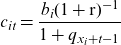
 \begin{equation*}c_{it}=\frac{b_i(1+\textrm{r})^{-t}}{1+{_tq_{x_i}}}\end{equation*}
to a survivor fund with maturity t, for
 $t=1,2,\ldots,\omega-x_i$
, where
$t=1,2,\ldots,\omega-x_i$
, where
 $\omega$
is the assumed ultimate age,
$\omega$
is the assumed ultimate age,
 ${_tq_{x_i}}$
is the probability that participant i dies before age
${_tq_{x_i}}$
is the probability that participant i dies before age
 $x_i+t$
, and r is the yearly discount rate (assumed to be constant, for simplicity). The total amount invested at time 0 is thus equal to
$x_i+t$
, and r is the yearly discount rate (assumed to be constant, for simplicity). The total amount invested at time 0 is thus equal to
 \begin{equation*}c_i=\sum_{t=1}^{\omega-x}c_{it}.\end{equation*}
With the proposed strategy, participant i is sure to receive at least the amount
 $b_i/(1+{_tq_{x_i}})$
if he or she is still alive at age
$b_i/(1+{_tq_{x_i}})$
if he or she is still alive at age
 $x_i+t$
. This amount tends to
$x_i+t$
. This amount tends to
 $b_i/2$
as t approaches
$b_i/2$
as t approaches
 $\omega-x_i$
, the remaining part of benefit coming from mortality credits. In this first strategy, participants abandon the amount
$\omega-x_i$
, the remaining part of benefit coming from mortality credits. In this first strategy, participants abandon the amount
 $c_i$
at time 0 and beneficiaries continue to receive mortality credits after participant’s death, until time
$c_i$
at time 0 and beneficiaries continue to receive mortality credits after participant’s death, until time
 $\omega-x_i$
, which may not be desirable.
$\omega-x_i$
, which may not be desirable.
Another possibility is to renew membership in one-year survivor funds over time intervals (0,1), (1,2),
 $\ldots$
, investing each year the amount of contribution providing the expected benefit
$\ldots$
, investing each year the amount of contribution providing the expected benefit
 $b_i$
targeted by participant i in case of survival. This means that the contribution
$b_i$
targeted by participant i in case of survival. This means that the contribution
 $c_{it}$
to the survivor fund running over time interval
$c_{it}$
to the survivor fund running over time interval
 $(t-1,t)$
is
$(t-1,t)$
is
 \begin{equation*}c_{it}=\frac{b_i(1+\textrm{r})^{-1}}{1+q_{x_i+t-1}}\end{equation*}
Under this second strategy, participant i is still sure to receive at least the amount
 $b_i/(1+q_{x_i+t-1})$
if he or she is still alive at age
$b_i/(1+q_{x_i+t-1})$
if he or she is still alive at age
 $x+t$
. Again, this amount tends to
$x+t$
. Again, this amount tends to
 $b_i/2$
as t approaches
$b_i/2$
as t approaches
 $\omega-x_i$
, the remaining part of benefit coming from mortality credits. But participant i is now free to manage his or her savings beyond the yearly contributions
$\omega-x_i$
, the remaining part of benefit coming from mortality credits. But participant i is now free to manage his or her savings beyond the yearly contributions
 $c_{it}$
to the survivor fund. In case of death at age
$c_{it}$
to the survivor fund. In case of death at age
 $x_i+k$
, future contributions
$x_i+k$
, future contributions
 $c_{i,k+t}$
,
$c_{i,k+t}$
,
 $t=1,\ldots,\omega-x_i-k$
, remain with participant’s estate. This is important since bequest motives often play an important role when planning retirement. Another possibility is to contribute
$t=1,\ldots,\omega-x_i-k$
, remain with participant’s estate. This is important since bequest motives often play an important role when planning retirement. Another possibility is to contribute
 $b_i$
each year to the survivor fund so that participant i is certain to get the targeted amount of benefit, supplemented with mortality credits. In the absence of bequest motive, participant i could invest his or her total savings in the survivor fund to get maximum extra return from mortality credits.
$b_i$
each year to the survivor fund so that participant i is certain to get the targeted amount of benefit, supplemented with mortality credits. In the absence of bequest motive, participant i could invest his or her total savings in the survivor fund to get maximum extra return from mortality credits.
Further analysis is required to compare the respective costs of these strategies to create lifelong income compared to conventional life annuities. The latter only grant mortality credits to survivors, thus increasing the income in retirement compared to survivor funds. But conventional annuities require expensive capital charges because of the guarantees they comprise. Survivor funds do not require any such charges but the benefits are not guaranteed. It has been shown that volatility can be lowered by enlarging the number of participants, but there always remains a risk that mortality credits are lower than expected. In that respect, minimum guarantees can be attractive to participants who could be protected against extreme situations where the number of survivors is much larger than expected.
Especially for small communities, the assumption of independence of remaining lifetimes may be violated. It is possible to take into account dependencies between the Bernoulli variables
 $I_i$
. However, the calculations of conditional expectations quickly become very complicated. The easiest way to account for dependence for small groups may be a conditional independence model, where the Bernoulli variables are independent given a common factor.
$I_i$
. However, the calculations of conditional expectations quickly become very complicated. The easiest way to account for dependence for small groups may be a conditional independence model, where the Bernoulli variables are independent given a common factor.
Conflicts of interest
There is no competing interests to declare.
Acknowledgements
The authors express their deepest gratitude to the Editor and two anonymous referees who provided them with accurate comments that greatly helped to improve this work compared to its initial version. In particular, one of the referees pointed out inaccuracies in the case where contributed amounts vary among participants. Example 4.1 and the accompanying discussion has been provided by him or her, offering us the chance to correct a previous version of our results. We are also grateful to Jan Dhaene and Daniel Linders for having provided us with a copy of their unpublished lecture notes “Foundations of Risk Measurement” where a thorough analysis of decomposition (2.4) can be found in Chapter 7. Michel Denuit gratefully acknowledges funding from the FWO and F.R.S.-FNRS under the Excellence of Science (EOS) programme, project ASTeRISK (40007517).
Supplementary material
To view supplementary material for this article, please visit https://doi.org/10.1017/asb.2022.13


 Open access