


INTRODUCTION AND AIMS
Given the ongoing and accelerating mass loss from the Greenland ice sheet (GrIS) and thus its contribution to global sea levels (Church and others, Reference Church and Stocker2013; Vaughan and others, Reference Vaughan and Stocker2013; Enderlin and others, Reference Enderlin2014), a growing body of research seeks to explore the drivers of this mass loss. Supraglacial lakes (SGLs) traditionally form annually within ice-surface topographic depressions (Echelmeyer and others, Reference Echelmeyer, Clarke and Harrison1991) within the GrIS's ablation zone, and are known to influence the loss in three ways. First, due to their lower albedo, SGLs enhance surface melting by 100–170% relative to the surrounding bare ice (Lüthje and others, Reference Lüthje, Pedersen, Reeh and Greuell2006; Tedesco and others, Reference Tedesco2012). Second, ~13% of SGLs (Selmes and others, Reference Selmes, Murray and James2011) drain in situ by hydrofracture in as little as 2 h and commonly in under 24 h. These rapid SGL drainage events deliver huge meltwater pulses to the ice-sheet bed, which can overwhelm the subglacial drainage system, drive down effective pressure, promote ice-bed decoupling and cause transient (hourly–weekly) ice speed-ups of up to 220% of background winter velocities (Das and others, Reference Das2008; Bartholomew and others, Reference Bartholomew2010; Banwell and others, Reference Banwell, Willis and Arnold2013, Reference Banwell, Hewitt, Willis and Arnold2016; Doyle and others, Reference Doyle2013; Tedesco and others, Reference Tedesco2013). Hydrofracture also creates surface-to-bed connections that can receive surface meltwater inputs for the remainder of the melt season, potentially sustaining ice-velocity increases over longer (monthly–seasonal) timescales, notably during any periods of high surface melting (Joughin and others, Reference Joughin2008; Shepherd and others, Reference Shepherd2009; Tedstone and others, Reference Tedstone, Nienow, Gourmelen and Sole2014). Finally, the opening of fractures during rapid SGL drainage results in surface meltwater reaching the colder ice within the ice-sheet body, heating it and thus promoting faster ice-deformation rates over long times (Phillips and others, Reference Phillips, Rajaram and Steffen2010, Reference Phillips, Rajaram, Colgan, Steffen and Abdalati2013).
While hydrofracture is recognised as an important contributor to the GrIS's mass loss, there is thought to be a discrepancy between its impact for different areas of the GrIS. Within ice-marginal, land-terminating regions (≤~1000 m a.s.l.), any mid-summer accelerations in ice velocity are typically offset by reduced late-summer (Bartholomew and others, Reference Bartholomew2010; Hoffman and others, Reference Hoffman, Catania, Neumann, Andrews and Rumrill2011; Sundal and others, Reference Sundal2011; van de Wal and others, Reference van de Wal2015) or winter velocities (Sole and others, Reference Sole2013). This is due to the evolution of the subglacial drainage system to higher hydraulic-efficiency channels, which can evacuate meltwater quickly, and in which there is a direct relation between effective pressure and increased discharge (Schoof, Reference Schoof2010; Chandler and others, Reference Chandler2013; Cowton and others, Reference Cowton2013; Andrews and others, Reference Andrews2014; Mayaud and others, Reference Mayaud, Banwell, Arnold and Willis2014). This therefore tends to produce either a net decrease (van de Wal and others, Reference van de Wal2008, Reference van de Wal2015; Tedstone and others, Reference Tedstone2015) or no net change in annual ice velocity within ice-marginal regions (Sole and others, Reference Sole2013). However, if hydrofracture can occur within the inland, land-terminating regions of the GrIS (>~1000 m a.s.l.), substantial uncertainty surrounds its implications for ice-sheet dynamics, notably since field measurements indicate that increased summer velocities are not offset by reduced wintertime ones (Doyle and others, Reference Doyle2014). It is hypothesised that this is because hydraulically-efficient subglacial drainage systems cannot form within inland regions due to the shallow ice-surface gradients, producing low hydraulic-potential gradients, and the thick overlying ice, producing high creep-closure rates (Bartholomew and others, Reference Bartholomew2011; Chandler and others, Reference Chandler2013; Meierbachtol and others, Reference Meierbachtol, Harper and Humphrey2013; Dow and others, Reference Dow, Kulessa, Rutt, Doyle and Hubbard2014, Reference Dow2015; Moon and others, Reference Moon2014). Instead, inefficient drainage here may persist year-round. This research therefore indicates that if SGLs can drain at higher elevations, the net overall slowdowns observed for the GrIS's marginal regions may not be observed further inland, potentially producing sustained mass loss into the future.
Meltwater volumes and the equilibrium line altitude are rising on the GrIS (Hanna and others, Reference Hanna2008; Howat and others, Reference Howat, de la Peña, van Angelen, Lenaerts and van den Broeke2013), forced by rising air temperatures (Box and others, Reference Box, Yang, Bromwich and Bai2009; Hanna and others, Reference Hanna, Mernild, Cappelen and Steffen2012) and the increasing frequency of negative summer North Atlantic Oscillation indices (Fettweis and others, Reference Fettweis, Tedesco, van den Broeke and Ettema2011, Reference Fettweis2013). This has led to observations of increasingly numerous SGLs at higher elevations, with greater areas, in the past decades (Sundal and others, Reference Sundal2009; Liang and others, Reference Liang2012; Howat and others, Reference Howat, de la Peña, van Angelen, Lenaerts and van den Broeke2013; Fitzpatrick and others, Reference Fitzpatrick2014). Given that warming is projected to continue over the coming century (Collins and others, Reference Collins and Stocker2013), SGLs are expected to continue their inland migration and to increase their areas (Leeson and others, Reference Leeson2015; Ignéczi and others, Reference Ignéczi2016). With these increasingly numerous SGLs that cover greater areas inland, enhanced surface ablation (due to the darker SGLs compared with bare ice) over greater portions of the GrIS could produce a more negative mass balance; moreover, these SGLs could affect ice dynamics if the water contained within them can reach the ice-sheet interior, perhaps by rapid in situ drainage if hydrofracture can occur. Although uncertain, the inland ice-dynamic speed-ups may be so pronounced that they exceed the net velocity slowdowns currently observed for ice-marginal regions.
It therefore becomes evident from the above discussion that to model the GrIS's future reliably, understanding is required of (i) the likely future locations of SGLs, (ii) whether these SGLs can drain rapidly and (iii) if they drain rapidly, how the subglacial hydrological system will respond to the basal meltwater deliveries. Towards fulfilling these requirements, some studies (Sundal and others, Reference Sundal2009; Liang and others, Reference Liang2012; Howat and others, Reference Howat, de la Peña, van Angelen, Lenaerts and van den Broeke2013; Fitzpatrick and others, Reference Fitzpatrick2014; Pope, Reference Pope2016) have linked the behaviour and properties of SGLs on the GrIS to climatic warming, with an assumption that understanding SGLs’ past response to warming will help inform knowledge of their future development. However, of these studies, only three elicited long-term trends in the evolution of SGLs in response to climatic warming, which have sequentially improved our understanding of SGLs. Howat and others (Reference Howat, de la Peña, van Angelen, Lenaerts and van den Broeke2013) studied SGLs over a 40-year period using Landsat data for 12 study sites across the GrIS, presenting the first long-term record of SGL evolution. However, their study only examined the elevation change of the uppermost 0.1 km2 of SGL area, and no information was presented on the total or individual SGL area changes or the changing area-elevation distributions over time. In addition, the temporal resolution of the data in Howat and others’ (Reference Howat, de la Peña, van Angelen, Lenaerts and van den Broeke2013) study was poor, with an average of only 2.25 images for each region between 1972 and 2000, although there were often more post-2000. Therefore, examining full regional changes to SGLs as well as using more images would likely have produced improved confidence in the study's conclusions. Fitzpatrick and others (Reference Fitzpatrick2014) fulfilled the necessity for higher temporal resolution data by using MODerate-resolution Imaging Spectroradiometer (MODIS) imagery for the 6500 km2 Russell Glacier region of south-west Greenland over 11 years (2002–12). However, using MODIS imagery meant that smaller SGLs (<0.0625 km2, i.e. below MODIS's one-pixel threshold reporting size) were omitted from their record, despite the potential for these SGLs to form fractures to the bed (Krawczynski and others, Reference Krawczynski, Behn, Das and Joughin2009). Liang and others (Reference Liang2012) presented a similarly valuable decadal-length study of SGLs in West Greenland using MODIS, showing how SGLs changed alongside melt indices, but did not examine SGLs’ inland advance over time. Finally, Sundal and others’ (Reference Sundal2009) study used MODIS data to improve our knowledge of the inland migration of SGLs, but this research was only for 4 years, meaning it was more difficult to elicit long-term trends. Collectively, these studies have produced a consistently improved understanding of the long-term evolution of SGLs on the GrIS, but because such studies are not more numerous, there remains significant uncertainty over the spatial and long-term (multi-decadal) response of SGLs to warming across the GrIS. In addition, if more studies linked the knowledge of the changing SGL distribution to meteorological data (such as surface temperatures or other melt indices), this could help inform debates surrounding the future progression of SGLs inland as temperatures rise over the next century, something currently unaccounted for in models (Church and others, Reference Church and Stocker2013).
Here, we extend this existing work by providing the most temporally extensive (1985–2016) and highest spatial resolution (30 m) existing examination of the response of SGLs to climatic warming within a ~6200 km2 sector of the north-west GrIS. Our two main aims are to: (i) elicit changes to the spatial distribution and coverage of SGLs in the region from 1985 to 2016; and (ii) evaluate these patterns within the context of regional surface-temperature changes. We choose a north-western sector of the GrIS because few studies have focused on SGLs in the region despite it including 19% of SGLs on the GrIS, the second largest frequency after the south-western area (Selmes and others, Reference Selmes, Murray and James2011), which has been the focus of previous research of this type (Sundal and others, Reference Sundal2009; Liang and others, Reference Liang2012; Fitzpatrick and others, Reference Fitzpatrick2014). The study site within the Qaasuitsup municipality of Greenland encompasses the outlets of Alison Gletscher, Illlullip Sermia and Cornell Glacier, and extends from the ice margin to just below 1800 m a.s.l. (Fig. 1).
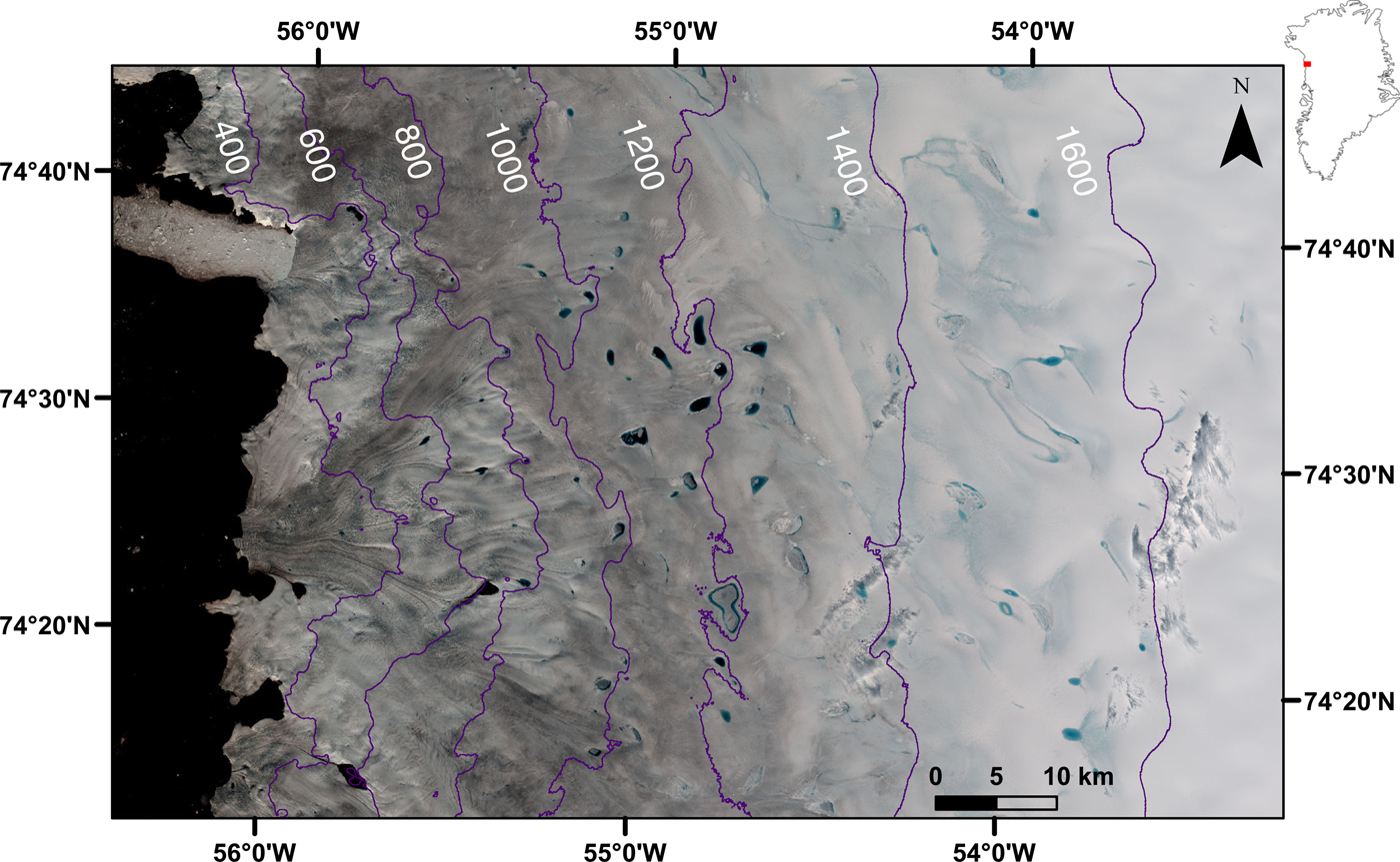
Fig. 1. The study site in north-west Greenland. Top-right inset shows the location of the study site (red square) within Greenland (black outline). The background is a false-colour red-green-blue (RGB) Landsat-8 Operational Land Imager (OLI) image (path: 019; row: 007) collected on 28 July 2015 (band 2 = red, band 3 = green, band 4 = blue). The purple lines indicate ice-surface elevation contours (in m a.s.l.) derived from the Greenland Ice Mapping Project (GIMP) DEM from Howat and others (Reference Howat, Negrete and Smith2014).
DATA AND METHODS
Satellite imagery data collection and pre-processing
Many studies of SGLs on the GrIS have used MODIS data (e.g. Selmes and others, Reference Selmes, Murray and James2011, Reference Selmes, Murray and James2013; Liang and others, Reference Liang2012; Fitzpatrick and others, Reference Fitzpatrick2014; Williamson and others, Reference Williamson, Arnold, Banwell and Willis2017). However, we opted for Landsat data because its finer 30 m spatial resolution (in the visible optical bands) allows much smaller SGLs to be resolved than with coarser resolution 250 m or 500 m MODIS data (i.e. minimum resolvable Landsat SGL size of 0.0009 km2 compared with a minimum MODIS resolvable SGL size of 0.0625 km2). It was deemed important to capture these small (<0.1 km2) SGLs in this study since they account for as much as 7.5% (Fitzpatrick and others, Reference Fitzpatrick2014) or 12% (Sundal and others, Reference Sundal2009) of the total SGL area during the mid-melt season, and because they may be able to initiate hydrofracture based on theoretical estimates (Krawczynski and others, Reference Krawczynski, Behn, Das and Joughin2009). In addition, the Landsat record extends further back than the MODIS one (i.e. 1972 for Landsat compared with 2000 for MODIS), allowing the long-term SGL evolution to be examined more comprehensively.
The Landsat images were acquired from the USGS Earth Explorer interface (http://earthexplorer.usgs.gov/). Since SGLs are highly transient, with an average 24-day lifespan (Johansson and others, Reference Johansson, Jansson and Brown2013), we only downloaded Landsat data for the years satisfying the condition of having at least four cloud-free images during July and August, maximising the probability of capturing all of the SGLs present within the region during the summer. While we realised that many small (<0.125 km2) SGLs form in mid- to late June, and may reach their maximum extents before the July images, the rapid drainage of these small lakes typically occurs in early to mid-July (Miles and others, Reference Miles, Willis, Benedek, Williamson and Tedesco2017; their Table 2), meaning that these lakes would usually not have disappeared from the ice-sheet surface prior to the July and August imagery; thus, they would have been included in our analysis. Any not included in the analysis were likely to have been small (both in number and in area), as is usually true early in the melt season, meaning that the overall impact on this study's results would be minimal. The images needed to be manually reviewed for cloud cover since the study site covered only a portion of an entire Landsat scene, preventing the use of image filtering using the interface's built-in cloud-cover algorithm, which could have led to omission of some valid images. There were 44 images meeting these criteria (Table S1), and they were from 1985, 1988, 1990 and 1994 (Landsat-5 Thematic Mapper (TM)), 2000, 2007 and 2009 (Landsat-7 Enhanced Thematic Mapper + (ETM+)), and 2014, 2015 and 2016 (Landsat-8 OLI). These images were level-1T products, meaning no radiometric correction was required. However, given that the image's geometric accuracy was crucial to ensure accurate reporting of the surface elevations of individual SGLs, each image was checked for geometric distortion against the 2016 image, which was regarded as geometrically rectified; geometric rectification was conducted in ArcGIS where the distortion from the 2016 reference image exceed one pixel (i.e. 30 m). This process involved fixing four control points on nunataks and then shifting any distorted images (with a polynomial transformation) to match the 2016 reference framework. Due to the Scan Line Corrector (SLC) failure on Landsat-7 ETM+ after 2002, the images from 2007 and 2009 could only be used to determine the maximum elevations of SGLs and not for any other analysis. All of the images were cropped to the study area using a georeferenced mask.
To ensure that the numbers of SGLs reported in each year were not a product of the images being available during only earlier or later parts of the melt season, we checked the image dataset for systematic bias towards earlier or later parts of the season. This was in addition to our inclusion of only the years where at least four images were available, as mentioned above. We recognise that comparing dates alone is only a first-order approximation for image bias towards specific periods of the season since it is plausible that early or late melt episodes within the melt season can occur. A one-way analysis of variance test was conducted after the image dates were converted to days of the year. This revealed that the yearly means of the image dates were not significantly different at the 90% confidence interval (F (9,34) = 0.590; p = 0.785) and that the standard deviations were similar between years (mean of standard deviations =17.3 days; range of standard deviations =13.7–23.0 days). Table S2 documents full comparisons of the yearly means and variance. We could therefore be confident that the variation in image dates between years would not considerably bias our study's results.
SGL identification and spatial analysis
SGL delineation technique
Various automatic methods exist for delineating SGLs, such as static band classification (Box and Ski, Reference Box and Ski2007; Arnold and others, Reference Arnold, Banwell and Willis2014; Banwell and others, Reference Banwell2014; Fitzpatrick and others, Reference Fitzpatrick2014), the Normalised Difference Water Index (e.g. Yang and Smith, Reference Yang and Smith2013; Moussavi and others, Reference Moussavi2016; Miles and others, Reference Miles, Willis, Benedek, Williamson and Tedesco2017), dynamic band thresholding (Selmes and others, Reference Selmes, Murray and James2011, Reference Selmes, Murray and James2013; Everett and others, Reference Everett2016; Williamson and others, Reference Williamson, Arnold, Banwell and Willis2017), a global and local classification approach (Yang and others, Reference Yang, Smith, Chu, Gleason and Li2015), image-histogram classification (Liang and others, Reference Liang2012; Howat and others, Reference Howat, de la Peña, van Angelen, Lenaerts and van den Broeke2013) and object-oriented classification (Johansson and Brown, Reference Johansson and Brown2013). While these automatic methods are less time-consuming compared with manual delimitation, they produce less accurate SGL boundaries even though the manual method is subject to some user bias (Leeson and others, Reference Leeson2013). Using relatively high-resolution Landsat imagery is likely to reduce this user bias more than if coarser imagery, such as that from MODIS, was used since the contrast between the darker SGL water and the brighter surrounding ice will not be altered by the low pixel resolution, as is the case with MODIS (Williamson and others, Reference Williamson, Arnold, Banwell and Willis2017).
We therefore selected to manually delineate SGL boundaries from the Landsat false-colour RGB composites, in line with previous studies (McMillan and others, Reference McMillan, Nienow, Shepherd, Benham and Sole2007; Hoffman and others, Reference Hoffman, Catania, Neumann, Andrews and Rumrill2011; Lampkin, Reference Lampkin2011; Lampkin and VanderBerg, Reference Lampkin and VanderBerg2011; Langley and others, Reference Langley, Leeson, Stokes and Jamieson2016). We adopted a set of uniform fixed guidelines, similar to Lampkin and VanderBerg (Reference Lampkin and VanderBerg2011), to ensure the consistency of our technique across all of the images: (i) rectilinear and curvilinear features were excluded since they were believed to represent supraglacial meltwater streams; and (ii) very small features where the SGL boundaries could not be discerned were omitted. For any SGLs that had ice floating over their centres, their areas were calculated for the water-covered area only rather than assuming that the ice-covered areas also represented water; this may have slightly underestimated total and individual SGL area, particularly since ice-covered SGLs tend to be larger than ice-free ones (Johansson and others, Reference Johansson, Jansson and Brown2013). We calculated the errors on the manually delineated areas following McMillan and others (Reference McMillan, Nienow, Shepherd, Benham and Sole2007); these error bounds were likely to be conservative since their method assumes that, for each pixel, the area is either overestimated or underestimated, when a combination of the two is more likely. From the individual SGL polygons, a binary (SGL and non-SGL) mask was created for each image, and then these masks were superimposed for each year to produce a maximum extent of the SGLs observed across all of the images in July and August of that year (Fig. S1). We acknowledge that the ‘maximum extent’ could not capture all of the water present on the ice-sheet surface at any point within the melt season, but simply represented a best estimate of this value.
Derivation of annual SGL metrics
From the maximum extent masks of SGLs within July and August from all of the available imagery each year, various metrics relating to the SGLs could be calculated. To calculate the elevations of SGLs for all of the years, we used the GIMP DEM (Howat and others, Reference Howat, Negrete and Smith2014). We used Howat and others’ (Reference Howat, Negrete and Smith2014) error bound of ±12.7 m for the surface-elevation measurements, which was calculated with the RMSD between the GIMP measurements and surface measurements from the Ice, Cloud and land Elevation Satellite (ICESat). Elevations were taken at SGL centroids, and we used nine discrete elevation bands at 200 m increments to investigate SGLs’ altitudinal variation over time. We note that using the same DEM, which was derived over the period 2003–09, for the entire study period may have introduced errors due to thinning of the north-western GrIS in 1992–2002 (Zwally and others, Reference Zwally2005), 1997–2003 (Krabill and others, Reference Krabill2004), 2003–07 (Pritchard and others, Reference Pritchard, Arthern, Vaughan and Edwards2009; Zwally and others, Reference Zwally2011), and 2001–14 (Helm and others, Reference Helm, Humbert and Miller2014; McMillan and others, Reference McMillan2016). This indicated that surface elevations in 1985–2007 were likely to have been underestimated, while those in 2007–16 were likely to have been overestimated. However, the overall magnitude of these errors was tens of metres, which was not sufficiently high to alter the conclusions of the study.
Total SGL area, and the distribution of SGL area by elevation band, was also derived by integrating the individual SGL areas across the (relevant portions of the) image. To derive SGL volume data, we used an empirically derived SGL area–volume scaling relationship rather than a more complex empirical depth-reflectance technique (Box and Ski, Reference Box and Ski2007; Fitzpatrick and others, Reference Fitzpatrick2014), or a physically-based approach applied to the image surface-reflectance data (Sneed and Hamilton, Reference Sneed and Hamilton2007; Georgiou and others, Reference Georgiou, Shepherd, McMillan and Nienow2009; Morriss and others, Reference Morriss2013; Arnold and others, Reference Arnold, Banwell and Willis2014; Banwell and others, Reference Banwell2014; Ignéczi and others, Reference Ignéczi2016; Langley and others, Reference Langley, Leeson, Stokes and Jamieson2016; Moussavi and others, Reference Moussavi2016; Pope, Reference Pope2016; Pope and others, Reference Pope2016; Williamson and others, Reference Williamson, Arnold, Banwell and Willis2017). We opted for this simple SGL area–volume scaling relationship since previous work indicates a strong and significant positive linear relationship between SGL area and volume (Box and Ski, Reference Box and Ski2007; Georgiou and others, Reference Georgiou, Shepherd, McMillan and Nienow2009; Morriss and others, Reference Morriss2013; Williamson and others, Reference Williamson, Arnold, Banwell and Willis2017). While such linear relationships do not always best represent the relationship between SGL areas and volumes (Williamson and others, Reference Williamson, Arnold, Banwell and Willis2017) and may not apply for the higher ice-surface elevations (where SGLs may be shallower due to the smaller ice-surface depressions), the errors derived from applying this simple relationship would be consistent across the study period. To derive the scaling relationship, we used SGL area and volume data from Box and Ski (Reference Box and Ski2007) and Georgiou and others (Reference Georgiou, Shepherd, McMillan and Nienow2009) (Fig. S2). From these data, we obtained a strong positive correlation between SGL area and volume (r = 0.931; p < 0.001), with SGL area explaining ~87% of the variance in SGL volume (R 2 = 0.867; p < 0.001). We then scaled SGL area to volume using the equation of the linear regression line (Fig. S2):
 $${\rm SGL}\,{\rm volume}\,(\times \; {10^6}\,{\rm m}^3) = 4.7105 \times {\rm SGL}\,{\rm area}\,({\rm k}{\rm m}^2).$$
Surface-temperature data collection
To link the observed changes in the spatial distribution of SGLs over the study period to climatic forcings, we used two surface-temperature datasets as proxies: for the period 2000–16, monthly surface-temperature data for the region were derived from MODIS; however, since these data were unavailable prior to 2000, for the period 1873–1999, nearby automatic weather station (AWS) data were used. Ideally, we would have used the same data for the entire study period, but since MODIS data were collected locally to the region (and so had less error associated with them), we used these data where they were available, instead of using AWS data for the entire period. We required the long-term AWS data to derive to a baseline 20th-century temperature, which would allow the calculation of the surface-temperature anomaly for our study period by comparing the surface-temperature value for each year against the baseline. The baseline was derived as the average of the summer surface temperature as measured with the AWS data from 1901–2000. We used these surface-temperature anomalies as proxies for total meltwater volume production in different years, but note that surface runoff is a product not only of surface temperatures but also of a suite of other factors, including accumulation rates and incoming solar radiation; this may have impacted the total variance explained by the surface-temperature anomalies.
MODIS temperature data
The MOD11C3 Land Surface Temperature, acquired by MODIS's Terra satellite, was selected since it provides monthly global composited and averaged temperature values in a 0.05° × 0.05° (i.e. 5600 m × 5600 m) latitude/longitude climate modelling grid. These data were downloaded manually for July and August from 2000–16 from the USGS's LPDAAC Data Pool (https://lpdaac.usgs.gov/data_access/data_pool/). Raw digital numbers (dn) were then extracted from a 9 × 17-point grid over the study area and averaged to produce a monthly mean temperature within the study region. Surface temperature was obtained with:
 $$T\; = (dn\; \times \; sf) - 273.15,$$
where T was surface temperature (in °C), sf was the data scale factor (0.02), and 273.15 was used to convert from Kelvin to degrees Celsius.
Weather station temperature data
Monthly air temperature data were available for ten AWSs around the periphery of the GrIS, with two in north-west Greenland proximal to the study site: one at Pituffik (number 4202) and a second at Upernavik (number 4211) (Cappelen and others, Reference Cappelen, Vinther, Kern-Hansen, Laursen and Jørgensen2015). To determine which of the AWS data were most representative of the weather at the study site, we downloaded data for these two AWSs from the Danish Meteorological Institute (http://research.dmi.dk/data/) for July and August for the period 1873–2015 (at Pituffik) and 1873–2014 (at Upernarvik). The AWS data were averaged for July and August and then compared against the average July and August surface temperatures derived from MODIS (see the section ‘MODIS temperature data’) during the overlapping years (2000–15 for Pituffik or 2000–14 for Upernarvik). We found that data from Upernavik (r = 0.772; p = 0.01; R 2 = 0.596) produced a better correlation and explained more of the variance in the MODIS data than the data from Pituffik (r = 0.555; p = 0.260; R 2 = 0.308) and so these data were used for the period 1985–99 (Fig. S3). We used the linear regression relationship (y = 0.0927(x) − 7.5548) from the AWS-to-MODIS temperature relationship to scale the 1873–1999 AWS data to ensure consistency with the MODIS values for the 2000–16 period. We calculated the standard error of the estimate, which measures the accuracy of measurements derived from a linear regression line, to provide error bounds on the 1873–1999 AWS data; since the MODIS data are effectively ground-truth data, we did not calculate error bounds for them.
Statistical analyses
We used four statistical techniques: (i) the area-weighted arithmetic mean to determine the mean elevation of SGLs for each measurement year; (ii) the Pearson's product-moment correlation coefficient (r) to assess the strength and nature of linear association between the measurement year and SGL metrics, and between summer surface-temperature anomalies and SGL metrics; (iii) the coefficient of determination (R 2) to quantify the extent to which surface-temperature anomalies explained the variance in SGL characteristics, and; (iv) multiple linear regression. Multiple linear regression involved setting the maximum areal extent of SGLs across the whole region as the response variable and then modelling the relationship between this variable and three explanatory variables. The three explanatory variables were the maximum areal extent of SGLs within the low, medium and high elevation bands (corresponding to <600 m a.s.l., 600–1199 m a.s.l. and ≥1200 m a.s.l., respectively). The standardised beta coefficients (β) were used to indicate the number of standard deviations from the mean by which the response variable changes for an increase in the explanatory variable by an increment of one standard deviation from the mean. It thus denoted the relative contribution of each explanatory variable to the response variable, and therefore indicated the extent to which changes to the maximum areal extent of SGLs within the three elevation bands produced the changes to maximum SGL extent observed across the region.
Prior to the statistical analysis, we conducted a series of assumption checks to provide high confidence in the results derived from the analysis. Our method involved: (i) checking for linearity of relationships and the presence of notable outliers by qualitatively assessing scatterplots; (ii) checking the data normality using the Shapiro–Wilk test; (iii) verifying that there was no autocorrelation with the Durbin–Watson statistic; and; (iv) in the case of multiple regression, testing for collinearity by calculating r values for the independent variables (Weisberg, Reference Weisberg2005). Any datasets failing these tests were discarded before further analysis. For all of the statistical tests, because of the small sample size in the study, we set the confidence interval at 90%, equivalent to a probability indicator (p) of 0.1. We also identified test results that were statistically significant with higher confidence intervals (i.e. 95% or 99%, p = 0.05 or 0.01, respectively).
RESULTS
Changes to the spatial distribution and coverage of SGLs
SGL elevation
Two years (2007 and 2009) were affected by the SLC failure on Landsat-7, meaning only the maximum SGL elevation could be ascertained for them. An average of 1014 SGLs (total number across all years = 8115, average SGL area across all years = 0.15 km2) was identified for each year from the eight maximum SGL extent images unaffected by the SLC failure (Table 1).
Table 1. Number, size and total area of the SGLs (including those that would not have been recorded by MODIS, i.e. <0.125 km2 in area) identified over the years of the study period.

Maximum SGL elevation increased by 418 m between 1985 (1252 m a.s.l.) and 2016 (1670 m a.s.l.), with the maximum observed elevation being 1672 m a.s.l. in summer 2015 (Figs 2, 3a). This long-term trend was confirmed by a strong correlation (r = 0.960; p = 0.000). Table 2 shows that the maximum elevation of SGLs changed at a rate of 13.5 m a−1; however, this rate was nearly three times higher in 2000–16 compared with 1985–99. The area-weighted SGL mean elevation also increased by 299 m between 1985 (817 m a.s.l.) and 2016 (1116 m a.s.l.), which is of a similar magnitude but ~100 m less than the increase to maximum SGL elevation. Again, a strong correlation (r = 0.935; p = 0.001) was associated with the SGL progression to higher mean elevations. The rate of change to the area-weighted mean elevation was similar (<5% different) to that observed for maximum SGL elevations over the entire period, with a similarly accelerated rate of more than double after 2000 compared with beforehand (Table 2).
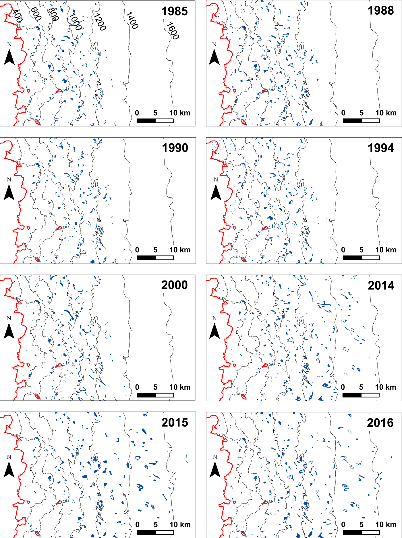
Fig. 2. Spatial distribution of SGLs across the study region for the 8 years unaffected by the SLC failure. The blue polygons represent maximum annual SGL extents, the red line shows the GrIS margin, and the black lines show ice-surface elevation contours (in m a.s.l.) from Howat and others (Reference Howat, Negrete and Smith2014). Contours are only labelled on the 1985 panel, but are consistent for all years. The total areal extent of each panel is equivalent to that shown in Figure 1.

Fig. 3. Changes to SGL metrics in 1985–2016: (a) maximum SGL elevation, (b) area-weighted mean SGL elevation, (c) maximum areal SGL extent across the whole region, (d) maximum areal SGL extent at low surface elevations, (e) maximum areal SGL extent at medium surface elevations, (f) maximum areal SGL extent at high surface elevations, and (g) maximum volumetric SGL extent across the whole region. Blue solid lines are shown to connect the data points, while red dashed lines show ordinary least-squares (OLS) linear regression lines. Significant r and R 2 values at above the 95% confidence interval (p < 0.05) are highlighted in bold italicised text on each panel. Black error bars for SGL areas and volumes are derived according to the section ‘SGL delineation technique’ and black error bars for elevations are derived according to the section ‘Derivation of annual SGL lake metrics’.
Table 2. The rates of change to annual SGL metrics within the study region over the full (t 1 + t 2), early (t 1), and late (t 2) periods, as well the relative rate of change (t 2/t 1) from the early to late periods.

SGL coverage
The maximum areal extent of SGLs nearly doubled over the 32-year period from 45.1 to 87.1 km2, with a maximum extent of >90 km2 in 2015 (Table 1 and Fig. 3c). A strong positive correlation (r = 0.883; p = 0.004) confirmed this relationship. In addition, individual SGLs tended to grow in size towards the end of the study period, with typically higher mean sizes across the whole region (mean = 0.13 km2 pre-2000 compared with mean = 0.15 km2 post-2000, although mean size in 2016 was much higher at 0.27 km2) and maximum SGL sizes (mean = 2.28 km2 until 2000 compared with mean = 3.50 km2 in 2014, 2015 and 2016) (Table 1). Within the later period (2014–16), we observed increasing variability in the size of the identified SGLs; for example, even though in 2015 the total regional SGL area was higher than in 2016 (95 km2 in 2015 compared with 87 km2 in 2016), the maximum individual SGL area was higher in 2016 (4.1 km2 in 2016 compared with 2.9 km2 in 2015). The rate of increase to the maximum areal extent accelerated more than fourfold from 0.53 km2 a−1 (1985–99) to 2.13 km2 a−1 (2000–16) (Table 2). Since the SGL volumes were derived using a linear regression relationship, the changes to SGL volumes mirrored those to SGL areas: volumes approximately doubled from ~45 × 106 m3 in 1985 to ~90 × 106 m3 in 2016, with a statistically significant (r = 0.883; p = 0.004) rate of change (1.35 × 10⁶ m3 a−1) over the entire period, with a fourfold accelerated rate of change post-2000 (Table 2). These changes were primarily driven by increases to SGL areas and volumes within the high elevation bands, notably those ≥1200 m a.s.l. (Fig. 4). For example, SGL area within the 1200–1399 m a.s.l. band remained approximately constant until 2014, when there were notable increases here, as well as large increases to SGL areas within the ≥1400 m a.s.l. elevation bands (Fig. 4).

Fig. 4. Maximum areal (y 1-axis) and volumetric (y 2-axis) regional extent of SGLs within individual 200 m ice-surface elevation bands (cf. Fig. 2) over the study period. Black error bars for SGL areas and volumes are derived according to the section ‘SGL delineation technique’.
In addition, we identified many SGLs (mean = 221 per image; maximum = 307 in 1990; minimum = 157 in 1985) under 0.125 km2 in size (i.e. those unresolvable by MODIS depending on whether one or two MODIS pixels can be confidently regarded as a SGL (Selmes and others, Reference Selmes, Murray and James2011, Reference Selmes, Murray and James2013; Fitzpatrick and others, Reference Fitzpatrick2014; Williamson and others, Reference Williamson, Arnold, Banwell and Willis2017)). These SGLs represented relatively high proportions of the total regional SGL area (mean = 12.3%, equivalent to an area of 7.7 km2, with consistently >5% coverage relative to the total) (Table 1).
The individual 200 m a.s.l. elevation bands were combined into broader categories of low (<600 m a.s.l.), medium (600–1199 m a.s.l.) and high (≥1200 m a.s.l.) surface elevations to assess the wider-scale patterns. At low elevations, the maximum areal extent of SGLs did not change significantly over the period (r = −0.554; p = 0.155), even though there was a large (almost quadruple) range in the area from 4.30 km2 (in 1990) to 16.50 km2 (in 1988) and an apparent downwards trend (Figs 2, 3d). A similar pattern was observed at medium elevations (Figs 2, 3e): while there appeared to be an upwards trend, this could not be confirmed statistically (r = 0.571; p = 0.139). There was also less relative variation for the medium elevations between the minimum (34.9 km2 in 1985) and maximum (44.8 km2 in 1994) values over the study period. The rates of change at the low and medium elevations were also not noteworthy, especially for the low elevations, with the rate showing almost no change during the study period (Table 2). Contrasting with the observations for low and medium elevations, the maximum areal extent at high elevations showed significant (r = 0.932; p = 0.000) increases of >2750% over the period from 1.21 km2 in 1985 to 34.9 km2 in 2016 (Figs 2, 3f). This change comprised only small changes to the maximum areal extent of SGLs at high elevations between 1985 and 1999 (with values always remaining below 6 km2), but substantial increases post-2000 (although data were only available for the years 2014–16), with values consistently above 30 km2 in the most recent (2014, 2015 and 2016) summers (Fig. 3f). This therefore produced a very high rate of increase in the later period (1.88 km2 a−1 in 2000–16) compared with the earlier one (0.23 km2 a−1 in 1985–99), representing an eightfold and nearly an order of magnitude increase (Table 2). Examining the 200 m a.s.l. elevation banding revealed that this late (post-2010) acceleration was attributable to increases in the SGL area within the 1200–1399 m a.s.l. elevation band, and the unprecedented appearance of SGLs within the 1400–1599 m a.s.l. and ≥1600 m a.s.l. elevation bands (Figs 2, 4).
Relative to the total SGL area change of 42.0 km2 over the study period, changes to the SGL area at the higher elevations accounted for a greater portion (80.1% or 33.7 km2) of the total change than changes to SGLs at the medium (23.8% or 10.0 km2) or low elevations (−3.81% or −1.60 km2). Multiple-regression analysis confirmed these patterns: the maximum areal extent of SGLs was predominantly influenced by the area at high elevations (β = 0.936; p = 0.000) rather than at medium (β = 0.214; p = 0.000) or low elevations (β = 0.202; p = 0.000). The same β values were obtained for the changes to regional SGL volumes for the differing elevation bands.
The influence of surface-temperature changes on SGLs
Changes to regional surface temperature
Recent (1985–2016) changes to surface temperatures in the region were contextualised against the long-term (1873–2016) record (Fig. 5). This time series showed that surface-temperature anomalies increased by 4.24°C from −2.02°C in 1873 to +2.22°C in 2016, and, in ~1945, switched from being generally negative to generally positive (Fig. 5). This long-term warming trend was statistically significant (r = 0.505; p = 0.000). The 10-year moving average showed that the increase in surface-temperature anomalies was most substantial post-2000 as the rate of change in 2001–16 (0.148 °C a−1) was two orders of magnitude greater than that in 1873–2000 (0.007°C a−1). Moreover, surface-temperature anomalies during the 21st century were the highest on record, with the average anomaly in 2000–16 (+1.90°C) being more than double the average in any previous decade, and comparing with the average from 1873 to 1999 of −0.18°C. Finally, 9 of the 10 warmest years in the entire record occurred during the 21st century (Fig. 5). Table 3 shows the summer surface-temperature anomalies for the years of this study: the highest values occurred in 2007, 2009, 2015 and 2016; the lowest were in 1990 and 2000. The mean and minimum surface-temperature anomalies for the years of this study were +1.27 and −0.73°C, respectively, but there was some spread in the data (σ = 1.39°C) (Table 3).
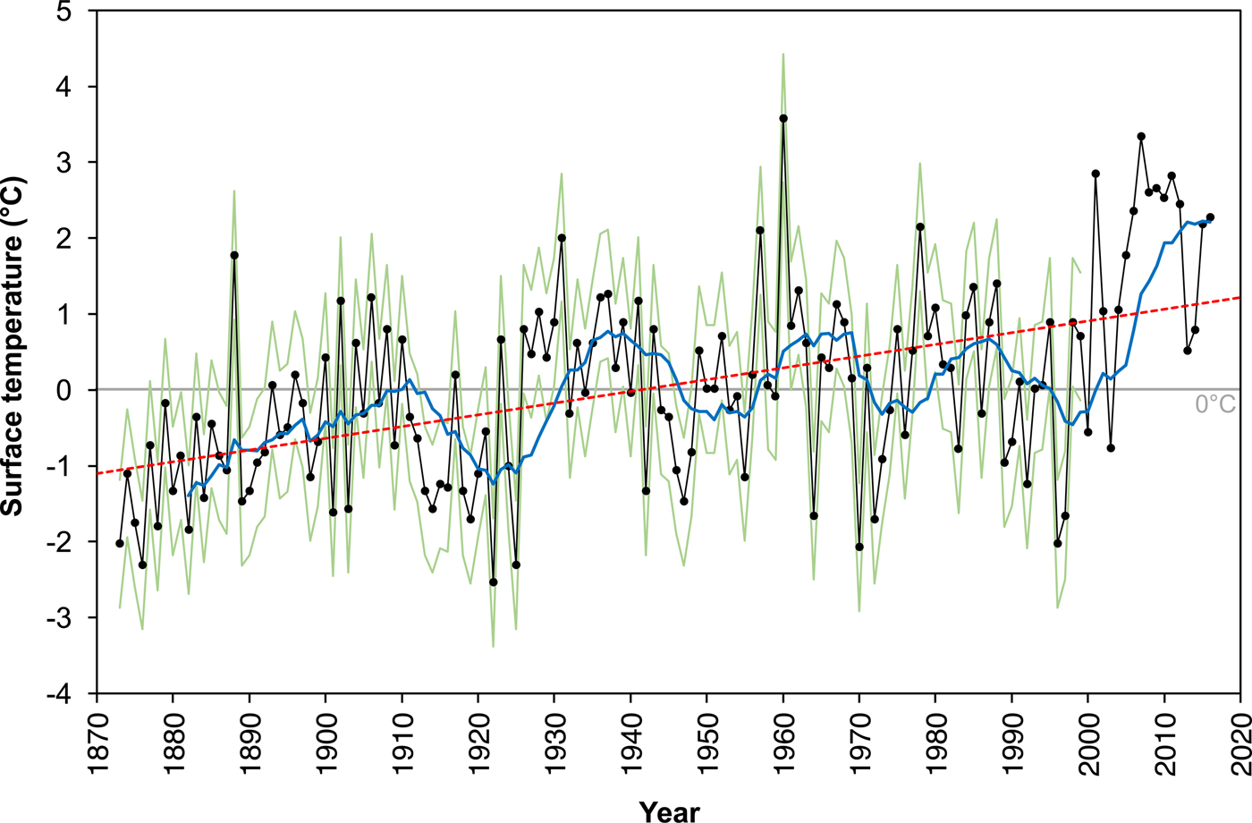
Fig. 5. Mean summer (July and August) surface-temperature anomalies (black line, with black circles showing individual yearly values) from 1873 to 2016 relative to the 20th-century baseline. Values from 1873 to 1999 are derived from AWS data (see the section ‘Weather station temperature data’), while those in 2000–16 are derived from MODIS data (see the section ‘MODIS temperature data’). The blue line shows the 10-year moving average for surface-temperature anomalies. The green lines show the positive and negative error bounds for the weather station data in 1873–1999 (derived according to the section ‘Weather station temperature data’); error bars are not shown for the 2000–16 MODIS data. The red dashed line is an OLS linear regression line (y = 0.0155x − 1.1182; r = 0.505; R 2 = 0.255; p = 0.000) to show the upward trend in surface-temperature anomalies over the period. The grey horizontal solid line shows the 0°C surface-temperature anomaly.
Table 3. Mean summer (July and August) surface temperatures and surface-temperature anomalies in °C (relative to the 20th-century baseline value) for the years of data used in this study.

The influence of surface temperatures on SGL elevation
When summer surface-temperature anomalies were highest, the maximum elevation of SGLs was also higher: for example, the extremely high SGL elevation values (relative to a mean maximum elevation over the 1985–2016 period of 1471 m a.s.l.) of 1578 m a.s.l. in 2007, 1578 m a.s.l. in 2009, 1672 m a.s.l. in 2015 and 1670 m a.s.l. in 2016 were accompanied by high positive surface-temperature anomalies of +3.34, +2.65, +2.18 and +2.28°C, respectively (Fig. 6a). Similarly, the extremely low values when maximum SGL elevations were only 1363 m a.s.l. in both 1990 and 2000 were accompanied by the most negative surface-temperature anomalies (−0.73 and −0.61°C, respectively). These patterns were confirmed by a moderate and statistically significant positive correlation (r = 0.637; p = 0.048) between maximum SGL elevation and surface-temperature anomalies. Furthermore, linear regression indicated that the surface-temperature anomalies explained 40.6% of the variance in maximum SGL elevations (R 2 = 0.406; p = 0.048) (Fig. 6a).

Fig. 6. The relationship between the summer (July and August) surface-temperature anomalies in 1985–2016 and (a) maximum SGL elevation, (b) area-weighted mean SGL elevation, (c) maximum areal SGL extent across the whole region, (d) maximum areal SGL extent at low surface elevations, (e) maximum areal SGL extent at medium surface elevations, (f) maximum areal SGL extent at high surface elevations, and (g) maximum volumetric SGL extent across the whole region. Red dashed lines show OLS linear regression lines. Significant r values at above the 90% confidence interval (p < 0.1) are highlighted in bold italicised text on each panel.
However, there was no statistically significant relationship (r = 0.471; p = 0.239) between surface-temperature anomalies and the area-weighted mean SGL elevation (Fig. 6b). This was despite the mean elevation of SGLs being at its maximum (1164 m a.s.l.) during summer 2015, which had the second largest surface-temperature anomaly (+2.18°C), and the 1990 and 2000 summers (with the most negative surface-temperature anomalies of −0.73 and −0.61°C, respectively) showing lower mean SGL elevations of 946 m a.s.l. and 895 m a.s.l., respectively (Fig. 6b).
The influence of surface temperatures on SGL coverage
The maximum regional areal extent of SGLs appeared to increase as the surface-temperature anomaly increased (Fig. 6c). For example, the maximum extent of SGLs in the summer with the most positive surface-temperature anomaly (2016, +2.28°C) was 42.1% greater than the mean of the maximum areal extents of SGLs over the entire study period (66.7 km2). Similarly, the maximum areal extent of SGLs in the summer with the most negative surface-temperature anomaly (1990, −0.73°C) was 32.2% smaller than the mean (66.7 km2) of the maximum areal extents over the study period. This pattern was confirmed by a moderate-strong positive correlation between maximum regional SGL area and the surface-temperature anomalies (r = 0.719; p = 0.045), with the surface-temperature anomalies explaining 51.7% of the variance (R 2 = 0.517, p = 0.045) in the maximum areal extent of SGLs (Fig. 6c). Due to the linear SGL area–volume scaling relationship, the same correlation and regression relationships existed for the regional SGL volume data (Fig. 6g).
Despite this, we found no clear relationship between summer surface-temperature anomalies and the maximum areal extent of SGLs within the low and medium elevation bands. This was confirmed by linear correlation analysis, which indicated that the relationship between the areal extent of SGLs at low and medium elevations and surface-temperature anomalies was not statistically significant: r = 0.144, p = 0.733 for low elevations, and r = 0.418, p = 0.300 for medium elevations, respectively (Figs 6d, e). By contrast, at high elevations, there was an apparent relationship between summer surface-temperature anomalies and the maximum areal extent of SGLs. Regression analysis confirmed the relationship between higher positive surface-temperature anomalies and the greater areal extents of SGLs at high elevations (r = 0.641; p = 0.087), with surface-temperature anomalies explaining 41.1% of the variance (R 2 = 0.411, p = 0.087) (Fig. 6f). During the summer with the highest positive surface-temperature anomaly (2016, +2.28°C), the SGL area at ≥1200 m a.s.l. accounted for 40.1% (34.9 km2) of the total SGL area (87.1 km2) across the region, nearly double the contribution of SGLs at these elevations (21.0%) to the overall maximum extents during the entire 1985–2016 period. During the summer with the most negative surface-temperature anomaly (1990, −0.73°C), SGL area ≥1200 m a.s.l. only accounted for 11.1% (5.02 km2) of total SGL area (45.2 km2), representing nearly half of the 1985–2016 mean value at these elevations derived from all of the maximum SGL extents.
DISCUSSION
Increasing and accelerating regional surface temperatures
Summer surface-temperature anomalies increased by 4.24°C in the study region from 1873 to 2016, with the most significant increases post-2000. This trend parallels that across the entire GrIS, which showed a similar (~1°C) albeit smaller warming trend over a comparable time period (1840–2007) (Box and others, Reference Box, Yang, Bromwich and Bai2009; Kobashi and others, Reference Kobashi2011). The difference between the values in north-west Greenland and those for the entire GrIS adds validity to the assumptions of non-uniform patterns of temperature change thought to occur across the GrIS (Hall and others, Reference Hall, Williams, Luthcke and Digirolamo2008; Hanna and others, Reference Hanna, Mernild, Cappelen and Steffen2012; Cappelen and others, Reference Cappelen, Vinther, Kern-Hansen, Laursen and Jørgensen2015). These findings indicate that studies modelling the GrIS's hydrology must account for this spatial unconformity in meteorological patterns, with attention given to ensuring that the past observations are reliably replicated by models before they are applied into the future.
SGL migration to higher inland elevations
The statistically significant increases to both the maximum and area-weighted mean elevations of SGLs over the study period (increases by 418 m and 299 m, respectively) indicate a tendency for SGLs to form progressively further inland over the study period, with an acceleration post-2000 (Table 1 and Figs 2, 3a, b). This elevation increase is of the same order of magnitude as previous observations elsewhere in Greenland (Howat and others, Reference Howat, de la Peña, van Angelen, Lenaerts and van den Broeke2013; Fitzpatrick and others, Reference Fitzpatrick2014), with Howat and others (Reference Howat, de la Peña, van Angelen, Lenaerts and van den Broeke2013) also noting an acceleration in 2000–12 compared with 1972–99. However, the annual rate of change to the maximum SGL elevation within our study region (13.5 m a−1) was double the rate (6.8 m a−1) within the adjacent basin in north-west Greenland studied by Howat and others (Reference Howat, de la Peña, van Angelen, Lenaerts and van den Broeke2013). This may be because the periods of study were different, since Howat and others (Reference Howat, de la Peña, van Angelen, Lenaerts and van den Broeke2013) only used data from before 2012, and there may have been notable increases since then. The rate we find is more akin to the rate (16.5 m a−1) observed by Fitzpatrick and others (Reference Fitzpatrick2014) for the Russell Glacier region of south-west Greenland, suggesting that there may be high variations in the rates of inland advance of SGLs across the GrIS. Since Howat and others’ (Reference Howat, de la Peña, van Angelen, Lenaerts and van den Broeke2013) study also used primarily Landsat data, as well as other medium-resolution satellite datasets, the regional differences that we observe cannot be attributed to the inability of their study to identify small SGLs at these higher elevations, which would have been the case with Fitzpatrick and others’ (Reference Fitzpatrick2014) use of MODIS data.
The influence of surface temperatures on SGL inland migration
The migration of SGLs to higher maximum elevations appears to have been driven by the increases to summer surface temperatures, matching the findings of previous work (Liang and others, Reference Liang2012; Fitzpatrick and others, Reference Fitzpatrick2014). Our analysis showed that surface temperature changes explained ~40% of the variance in maximum SGL elevations (Fig. 6a), likely because higher surface temperatures promote increased surface melting across greater portions of the GrIS (Howat and others, Reference Howat, de la Peña, van Angelen, Lenaerts and van den Broeke2013). Conversely, we found no relationship between surface-temperature anomalies and the area-weighted mean SGL elevation, showing that there is no tendency for SGLs to be present at higher mean elevations on the GrIS with increased temperatures (Fig. 6b). A possible explanation for this is that with higher surface temperatures, the statistically significant increases to the maximum SGL elevations are not so large that they bias the overall SGL elevation towards higher mean values. If imagery had been available from the extreme 2012 melt season (Noël and others, Reference Noël2016), further conclusions could have been reached on the influence of surface temperatures on SGL inland migration, and particularly SGLs’ response to such extreme values. Overall, Figure 6 shows that regional SGL characteristics cannot be inferred directly from surface temperature (and so surface melt intensity), indicating that there are likely to be other controls, such as the local glaciological characteristics (for example, the surface slope or the size of depressions) or hydrological characteristics (for example, the availability of meltwater or the patterns of its routing into lake basins) that control the evolution and morphology of SGLs within the study region. Furthermore, it is possible that using only surface temperatures, in the absence of other meteorological variables, cannot explain the observed variations, so if extra meteorological data had been included in the analysis, these may have been able to explain more of the observed interannual differences.
Intra- and inter-ice-sheet sector variations in SGL inland advance
Previous work has indicated that there is likely to be significant variations in the extent of inland migration of SGLs for different sectors of the GrIS (Howat and others, Reference Howat, de la Peña, van Angelen, Lenaerts and van den Broeke2013; Leeson and others, Reference Leeson2015; Ignéczi and others, Reference Ignéczi2016). Our study also demonstrates that even within specific sectors of the GrIS (by comparing our results with those from the nearby basin studied by Howat and others (Reference Howat, de la Peña, van Angelen, Lenaerts and van den Broeke2013)), there may also be marked variation in the rate of inland SGL migration. The observed Greenland-wide variations in the patterns of the extent of inland SGL progression (Howat and others, Reference Howat, de la Peña, van Angelen, Lenaerts and van den Broeke2013) are likely to be due to sector-specific variations in melt extent (Ohmura and Reeh, Reference Ohmura and Reeh1991; Abdalati and Steffen, Reference Abdalati and Steffen2001), topography (Ignéczi and others, Reference Ignéczi2016) and glacier dynamics (Rignot and Kanagaratnam, Reference Rignot and Kanagaratnam2006). The results of this study therefore indicate that a similar set of controls may apply within ice-sheet sectors as well as between them. This agrees with recent work indicating that within ice-sheet sectors, there can be high variation in the number and size of ice-surface depressions, resulting from local-scale variations in the controls on depression formation, such as basal sliding (Gudmundsson, Reference Gudmundsson2003; Ignéczi and others, Reference Ignéczi2016). We therefore suggest that caution may be needed if applying the inferences of past and present SGL inland progression from one region of the GrIS to the entire GrIS (e.g. Leeson and others, Reference Leeson2015) and/or if assuming that the patterns of SGL change observed in one location on the GrIS will be necessarily representative of the entire GrIS. Instead, we recommend that finer-scale regional and sector-specific results for SGL migration should be ascertained first and then incorporated into models of the future progression of SGLs on the GrIS.
Finally, it appears that an upper altitudinal limit to SGL elevation within this study region has not yet been reached – indeed the rates of SGL migration to higher elevations were most notable during the latter part of the study period. This result agrees with Ignéczi and others (Reference Ignéczi2016) who indicated that the upper limit to SGL formation in the region may be as high as ~3000 m a.s.l. With a continually warming climate (Collins and others, Reference Collins and Stocker2013), and assuming a constant rate of SGL inland migration, it seems plausible that SGLs will form at higher surface elevations in the region in the future, although verification must be undertaken to determine whether the trend observed in the later part of our study period is likely to continue into the future. It is impossible with this study's results to speculate on whether these higher-elevation SGLs will be capable of hydrofracture in the future. However, our work suggests that since SGLs are forming at progressively higher elevations and covering greater extents at these elevations, with accelerations to these rates over time, further research should be directed towards determining whether these SGLs will be able to drain rapidly and, if they can, how this will implicate the GrIS's future dynamics. This research might build on existing observational (remote sensing or field) studies of rapid SGL drainage by including an examination of some of the potential drivers of the hydrofracture process, as well by furthering theoretical modelling work.
Increases to the spatial coverage of SGLs
Alongside the migration of SGLs to higher elevations, our findings show that the maximum areal and volumetric extent of SGLs significantly increased over the study period, nearly doubling between 1985 and 2016, with notable accelerations during the 21st century. However, this trend was not uniform for all elevation bands, with the increases at low and medium elevations showing no statistically significant trend compared with the statistically significant increases at high elevations. The expansions to total SGL areas and volumes were therefore driven by changes at the highest elevations (as confirmed by multiple regression) rather than by changes for the entire ablation area. This result agrees with Sundal and others (Reference Sundal2009) and Liang and others (Reference Liang2012) who showed that increases to SGL extent at high elevations drove recent changes to total regional SGL area and volume in their studies.
Given this finding, we investigated whether SGLs for the low, medium and high elevation bands showed significant changes to their mean and maximum sizes over the study period (Fig. 7). The aim here was to determine whether it is likely that even within the early part of the study period, low- and medium-elevation SGLs reached similar sizes to those at these elevations later in the period; if so, this might indicate a regional topographic control on their size, similar to that observed elsewhere, such as in the Paakitsoq and Store Glacier regions of West Greenland (Williamson and others, Reference Williamson, Arnold, Banwell and Willis2017). We found no statistically significant change to mean SGL size at low elevations (r = 0.405, p = 0.319) over the study period, suggesting that a regional control might prevent their growth to larger areas. By contrast, the mean SGL size significantly increased over the study period for SGLs at medium (r = 0.840, p = 0.009) and high elevations (r = 0.617, p = 0.010). A similar pattern also existed for the maximum SGL sizes: there were no statistically significant changes at low elevations (r = 0.195, p = 0.644), but significant increases were observed at medium (r = 0.794; p = 0.019) and high elevations (r = 0.899, p = 0.002).

Fig. 7. Changes to SGL mean and maximum size over the study period divided into low (<600 m a.s.l; solid blue lines), medium (600–1199 m a.s.l.; dotted green lines) and high (≥1200 m a.s.l.; dashed red lines) elevation bands. Black error bars for SGL areas are derived according to methods in the section ‘SGL delineation technique’.
These findings show that SGLs at the lowest (<600 m a.s.l.) surface elevations remained approximately constant in size over the study period, indicating that during the earlier part of the study period, they might have already reached their maximum areas and could not grow larger later in the period. This probably indicates that the size of the depressions controlled their sizes, preventing the increased meltwater volumes during the later (post-2000) period from being accommodated within larger SGLs. While there may be small increases to SGL area and volume by enhanced SGL-bottom ablation (Lüthje and others, Reference Lüthje, Pedersen, Reeh and Greuell2006; Tedesco and others, Reference Tedesco2012), this shows that the bedrock topography and local sliding rates are a key control on SGL size (Thomsen and others, Reference Thomsen, Thorning and Braithwaite1988; Echelmeyer and others, Reference Echelmeyer, Clarke and Harrison1991; Gudmundsson, Reference Gudmundsson2003; Lampkin and VanderBerg, Reference Lampkin and VanderBerg2011; Johansson and others, Reference Johansson, Jansson and Brown2013). Consequently, statistically significant increases to the areas and volumes of these SGLs were impossible, so the increasing quantities of melt at low elevations during the later parts of the study period were presumably accommodated by the earlier drainage of SGLs, and the resultant opening of surface-to-bed connections, permitting the direct delivery of any future meltwater to the basal system for the remainder of the season (Colgan and others, Reference Colgan2011; Palmer and others, Reference Palmer, Shepherd, Nienow and Joughin2011; Banwell and others, Reference Banwell, Willis and Arnold2013, Reference Banwell, Hewitt, Willis and Arnold2016; Sole and others, Reference Sole2013; Tedstone and others, Reference Tedstone, Nienow, Gourmelen and Sole2014; Koziol and others, Reference Koziol, Arnold, Pope and Colgan2017). Meanwhile, in the earlier part of the study period, the basins at higher (≥600 m a.s.l.) elevations were likely to have been either empty or only partially filled, meaning that they were able to accommodate increasingly larger SGLs over the study period, shown by the increases to the mean and maximum sizes of SGLs at these elevations.
The influence of surface temperatures on increased SGL coverage
Our study shows that surface-temperature anomalies are a key driver of total SGL area and volume changes, being able to explain >50% of the variance in total SGL area and volume (Figs 6c, g). This agrees with previous work showing that SGLs cover larger areas inland during warmer years (Sundal and others, Reference Sundal2009; Liang and others, Reference Liang2012; Fitzpatrick and others, Reference Fitzpatrick2014). However, when we compared surface-temperature anomalies against total SGL areas at low, medium and high elevations, we found a significant correlation for only the high elevations (Figs 6d–f). This is similar to the findings of Liang and others (Reference Liang2012), which showed that there was strong variation only for SGLs >1050 m a.s.l. in response to melt intensity, and the results of Fitzpatrick and others (Reference Fitzpatrick2014), which also showed that maximum SGL areal extent >1400 m a.s.l. was strongly correlated with surface-temperature anomalies in June and July.
Our results show that at low and medium elevations, when surface temperature increases, total SGL area does not increase. This might be because the higher melt with higher temperatures is accommodated not by growth to the area of SGLs at these elevations but instead is accommodated by the earlier rapid SGL drainage or by the overflow of individual SGLs to feed downglacier moulins/crevasses; this prevents the water within depressions from reaching the maximum size of the depressions. This agrees with Liang and others (Reference Liang2012) who found a significant correlation between mean SGL cessation date (due to rapid SGL drainage) and melt intensity, and between SGL duration (with a lower duration if SGLs drain rapidly) and melt intensity, indicating that SGLs drain earlier to compensate for increased meltwater volumes. It is also plausible that the prevalence, by comparison with higher elevations, of crevasses and moulins at low and medium surface elevations (Catania and others, Reference Catania, Neumann and Price2008; Das and others, Reference Das2008; Colgan and others, Reference Colgan2011) allows the extra meltwater in high-temperature years to be routed directly to the bed instead of ponding supraglacially.
Contrastingly, at high elevations, the statistically significant correlation between surface-temperature anomalies and SGL area and volume indicates that extra melt can be accommodated by larger and/or more numerous SGLs. Given that there is such a strong correlation between the two variables, it is possible that: (i) high-elevation surface depression size does not (yet) control high-elevation SGL size; (ii) the lack of surface fractures compared with low and medium elevations means that surface water is stored within SGLs rather than being delivered directly to the bed; or (iii) high-elevation SGLs presently cannot drain rapidly by hydrofracture, meaning that with higher temperatures, total SGL area at these elevations instead continues to increase. The absence of rapid drainage may result from: (i) the lack of basal meltwater inputs to the subglacial drainage system elsewhere at high elevations (Stevens and others, Reference Stevens2015); (ii) the preclusion of rapid drainage due to the lack of surface crevasses at high elevations (Poinar and others, Reference Poinar2015); or (iii) the shallow ice-surface slopes at high elevations producing spatially expansive but shallow SGLs that cannot drain rapidly (Raymond and Nolan, Reference Raymond and Nolan2000). The use of a more robust SGL area–volume scaling relationship, such as a physically-based one (Sneed and Hamilton, Reference Sneed and Hamilton2007), would allow the third possibility to be investigated more fully than is possible with the simple SGL area–volume linear relationship used here. Although this study could not examine whether rapid drainage at these elevations will be able to occur in the future, if hydrofracture could initiate, it is possible that with increased meltwater volumes associated with higher future temperatures (Collins and others, Reference Collins and Stocker2013), which appear to be accelerating, SGL area at high elevations would not be correlated so strongly with surface-temperature anomalies.
Identification of small SGLs
SGLs <0.125 km2 in size (i.e. below MODIS's threshold reporting size) represented relatively high proportions of the regional SGL areal and volumetric extents. It is therefore evident that it is important to employ higher-resolution imagery to fully document past changes to SGL areas for different regions of the GrIS, meaning that studies based solely on MODIS (Sundal and others, Reference Sundal2009; Liang and others, Reference Liang2012; Fitzpatrick and others, Reference Fitzpatrick2014) may have omitted some information on past changes to the GrIS's hydrology, particularly if calculating total regional areal and volumetric SGL extents. With the increasing availability of higher spatial and temporal resolution satellite imagery such as that derived from the Sentinel-2 satellite (10 m spatial resolution and 4-day or better repeat times for Greenlandic latitudes), it will be possible to resolve much finer-scale changes to SGL metrics on the GrIS, including the identification of changes to supraglacial streams (Yang and Smith, Reference Yang and Smith2013). Ultimately, this will provide a more valuable record of the GrIS's ongoing response to climatic warming than was possible for previous decades, such as those examined here.
CONCLUSIONS
The potential future expansion of SGLs to higher surface elevations on the GrIS, and particularly the possibility of their rapid drainage at these elevations, has received recent attention because of its implications for the GrIS's future mass balance if the subglacial system within the interior regions cannot evolve to higher hydraulic efficiency. Ultimately, this could produce longer-term, persistent ice speed-ups that may even offset the presently observed ice-velocity slowdowns closer to the ice margin. Towards eliciting the future locations and potential drainage locations of SGLs on the GrIS, and for determining the ongoing response of the GrIS's hydrology to climatic warming, some studies have examined changes to patterns of SGLs over the past decade(s). However, existing research was either temporally limited to post-2000 and used coarse-resolution MODIS data (Sundal and others, Reference Sundal2009; Liang and others, Reference Liang2012; Fitzpatrick and others, Reference Fitzpatrick2014) or did not contextualise the observed changes to SGLs with surface temperature changes (Howat and others, Reference Howat, de la Peña, van Angelen, Lenaerts and van den Broeke2013). Here, we addressed these shortfalls by conducting the longest-term (1985–2016) and highest spatial resolution (30 m) study of the past response of SGLs, examining not only changes to SGL elevations but also regional SGL areal and volumetric extents, then comparing the observations with surface-temperature changes.
Our results showed that SGLs have advanced to higher maximum (+418 m) and mean (+299 m) elevations, with notable accelerations inland post-2000. In addition, the total regional SGL area and volume nearly doubled over the study period, again with large accelerations post-2000, which were driven by increases to the SGL area and volume at high (≥1200 m a.s.l.) surface elevations. Here, the maximum areal extent of SGLs increased by >2750% over the study period and these high-elevation changes could explain ~80% of the changes to the total regional SGL areal extent. The notable accelerations in the 21st century were mirrored by accelerations to surface temperatures (showing a two order of magnitude increase post-2000 compared with beforehand). These temperature changes could explain the higher maximum SGL elevation, as well as the total SGL coverage across the region and at high elevations; however, we found no significant relation between SGL areas at low and medium elevations and the surface temperature changes. This is likely because depressions at the low and medium elevations control SGL size, whereas SGLs at higher elevations have not yet grown to fill the large depressions; it may also reflect the prevalence of moulins and crevasses at the lower elevations, meaning that increased meltwater here is routed directly to the bed instead of ponding within depressions as at the high elevations.
Collectively, our results are concerning since they show an accelerating and significant response of the GrIS's hydrological system to past climatic warming, which may result from anthropogenic climate change (Collins and others, Reference Collins and Stocker2013). With the apparent continued accelerating inland progression of SGLs over the most recent period, as well as the increasing SGL areas and volumes at high elevations, there is an urgent need to understand whether rapid SGL drainage by hydrofracture will be able to occur at these elevations and, if it can, how it will implicate ice dynamics in the future. Further work should focus on identifying whether the notable changes in the later part of this study (i.e. 2014–16) represent an ongoing trend to determine their relation to climate change. Our study also shows that there appears to be significant intra-ice-sheet variation in the response of SGLs to climatic warming, suggesting that finer spatial scale studies for different sectors of the GrIS would be merited. Finally, if it were possible to link the locations of SGLs and their drainage patterns over many years or decades to changes in the subglacial drainage system structure and the resultant ice velocities, much greater insights might be provided into the likely response of increasingly inland regions of the GrIS to SGL formation and potential SGL drainage in the future. This could enable improved confidence in the forecasts of ice-dynamic loss from the GrIS and consequently its potential contribution to global sea levels over the coming century.
AUTHOR CONTRIBUTIONS
Both authors contributed equally to this work. Under the supervision of AGW, LAG conceived the study, designed the research and undertook the majority of the data processing. Results and interpretation were discussed by both authors. AGW wrote the manuscript and created the figures based on LAG's undergraduate dissertation for Part II of the University of Cambridge Geographical Tripos. AGW responded to comments from reviewers and revised the manuscript.
SUPPLEMENTARY MATERIAL
The supplementary material for this article can be found at https://doi.org/10.1017/aog.2017.31.
ACKNOWLEDGEMENTS
LAG received a Hugh Brammer Vacation Study Grant (Downing College, Cambridge) to conduct the majority of the research. AGW was in receipt of a UK Natural Environment Research Council PhD studentship awarded through the Cambridge Earth System Science Doctoral Training Partnership (grant number: NE/L002507/1). We are grateful to James Kirkham for commenting on an early draft of the manuscript. We thank Gabriel Amable for providing technical assistance with certain aspects of the image processing and Mal McMillan for answering our questions on calculating the errors associated with manually digitising SGLs. We also acknowledge Poul Christoffersen's and Gareth Rees’ preliminary suggestions during the study's conception. Finally, we thank two anonymous reviewers and the Scientific Editor, Allen Pope, for their thorough reviews that improved the manuscript.


 Open access