I. INTRODUCTION
In recent years, great interest was given to the realization of low-cost light antennas with high performances in order to extend their use to the public sector. Among the possible candidates, modulated metasurface antennas give interesting performances with a relatively low cost and complexity of production. Metasurfaces are two-dimensional structures consisting of sub-wavelength elements, printed over a grounded dielectric slab. By acting on the size, shape, and orientation of the printed elements, the metasurfaces are modulated. Several examples of such modulated metasurfaces have been designed and presented in the literature [Reference Fong, Colburn, Ottusch, Visher and Sievenpiper1–Reference Teniou, Roussel, Capet, Piau and Casaletti7].
The propagation of surface waves (SW) along metasurfaces can be controlled by introducing a modulation of the metasurfaces. In addition, a proper choice of the modulation parameters leads to the generation of radiated leaky-waves (LW) propagating away from the metasurface. Moreover, the metasurface modulation parameters can be used to control the properties of the generated LW (amplitude, phase, and polarization). In [Reference Teniou, Roussel, Capet, Piau and Casaletti7–Reference Teniou, Roussel, Capet, Piau and Casaletti9], a method for the generation of aperture field distributions using modulated tensorial metasurfaces was presented. In these articles, a wide range of radiation pattern was achieved with a validation using numerical simulations.
This paper is an extension of [Reference Teniou, Roussel, Capet, Piau and Casaletti9] for which feeder design and experimental results have been added. In Section II, the theoretical procedure for the generation of aperture field distributions using modulated metasurfaces presented in [Reference Teniou, Roussel, Capet, Piau and Casaletti7] is resumed. Section III presents the design procedure of the feeder as well as the geometrical parameters affecting the antenna matching. In Section IV, the aperture generation procedure is validated through numerical simulation of a single beam and a multi-beam metasurface antenna working at 12.25 and 20 GHz, respectively. Simulation results are compared with theoretical radiation patterns. Finally, a metasurface prototype, operating at the frequency f = 12.25 GHz, is manufactured and measured in Section V. Conclusions are drawn in Section VI.
II. FORMULATION
The general geometry is depicted in Fig. 1. A feeder excites a cylindrical surface wave propagating above a metasurface realized by printed conducting elements above a grounded dielectric substrate. The physical properties of the metasurface are described in terms of equivalent surface tensorial impedance  $\underline{\underline {Z_s}} $. This latter is defined as the ratio between tangential electric (E t) and the magnetic (H t) fields at the surface boundary S, namely:
 $$\left. {{\left. {{\bf E}_t({\bf {\rho} ^{\prime}})} \right \vert} _{{\bf {\rho} ^{\prime}} \in S} = \underline{\underline {{\bf Z}_{\bf s}}} {\bf \hat n} \times {\bf H}_t({\bf {\rho} ^{\prime}})} \right \vert _{{\bf {\rho} ^{\prime}} \in S} = \underline{\underline {{\bf Z}_{\bf s}}} {\bf J}({\bf {\rho} ^{\prime}}),$$
where  ${\bf {\rho} ^{\prime}} = {x}^{\prime}{\bf \hat x} + {y}^{\prime}{\bf \hat y}$ is a point on the antenna surface,
  ${\bf \hat n}$ is the vector normal to the surface S, and
  $\left. {{\bf J}({\bf {\rho} ^{\prime}}) = {\bf \hat n} \times {\bf H}_t({\bf {\rho} ^{\prime}})} \right\vert _{{\bf {\rho} ^{\prime}} \in S}$ is the equivalent surface current.

Fig. 1. Metasurface geometry and LW generation.
Under the assumption that the metasurface is composed of reciprocal and lossless materials, the surface impedance is a purely imaginary symmetric tensor [Reference Hoppe and Rahmat-Samii10]. Thus, equation (1) reduces to:
 $$\left[ {\matrix{ {E_1} \cr {E_2} \cr}} \right] = j\left[ {\matrix{ {X_{11}} & {X_{12}} \cr {X_{12}} & {X_{22}} \cr}} \right]\left[ {\matrix{ {J_1} \cr {J_2} \cr}} \right]$$
For this kind of structures, the dominant mode is a hybrid EH surface wave mode [Reference Bilow11]. The magnetic field above the metasurface will be of the general form [Reference Teniou, Roussel, Capet, Piau and Casaletti7]:
 $${\bf H}_t({\bf {\rho} ^{\prime}}) = I({\bf {\rho} ^{\prime}})\,e^{ - j{\bf k}^{{\bf sw}}({\bf {\rho} ^{\prime}}) \cdot {\bf {\rho} ^{\prime}}}{\bf \hat h}({\bf {\rho} ^{\prime}})$$
where I is the field amplitude,  ${\bf \hat h}$ is the magnetic field polarization unit vector,
  ${\bf k}^{{\bf sw}} = k_t^{sw} {\bf \hat k}^{sw}$ and
  $k_t^{sw} $ are the wave vector and the propagation constant, respectively.
The propagation constant  $k_t^{sw} $ is obtained using transverse resonance technique [Reference Bilow11, Reference Casaletti12]. It should be noted that
  $\underline{\underline {{\bf Z}_{\bf s}}} $ depends on the considered wavenumber and propagation direction, namely
 $${\bf k}^{{\bf sw}} = k_t^{sw} (\omega, \varphi )({\bf \hat x}\cos (\varphi ) + {\bf \hat y}\sin (\varphi )),$$
where k sw(ω, φ) is the wavenumber associated with the dominant mode propagating along the direction  ${\bf \hat k}_t^{sw} $ defined by the angle φ (Fig. 1) at the angular velocity ω.
A sinusoidal modulation of the surface reactance components along the direction of propagation leads to the generation of an infinite number of Floquet-modes [Reference Casaletti12]. We consider a reactance components variation of the form :
 $$X_{ij}(x) = \bar X_{ij}\left[ {1 + M_{ij}\cos \left( {\displaystyle{{2\pi} \over {p_{ij}}}x} \right)} \right],$$
where  $\bar X_{ij}$, M ij, and p ij are the average reactance, the modulation index and the periodicity of the ij component, respectively.
For small modulation indices, modes of order −1 are predominant [Reference Casaletti12]. Under this condition, LW can be generated if the quantity  $k_t^{sw} - (2\pi /p_{ij})$ is smaller than the free space propagation constant k 0. The generated LW will then have the following form [Reference Teniou, Roussel, Capet, Piau and Casaletti7]:
 $$\eqalign{{\bf E}_t^{LW} & = \left[ {\matrix{ {E_1^{LW}} \cr {E_2^{LW}} \cr}} \right] \cr & = j\left[ {\matrix{ {\displaystyle{{M_{11}} \over 2}{\bar X}_{11}J{}_1e^{ - j\displaystyle{{2\pi} \over {p_{11}}}x} + \displaystyle{{M_{12}} \over 2}{\bar X}_{12}J_2e^{ - j\displaystyle{{2\pi} \over {p_{12}}}x}} \cr {\displaystyle{{M_{21}} \over 2}{\bar X}_{21}J{}_1e^{ - j\displaystyle{{2\pi} \over {p_{21}}}x} + \displaystyle{{M_{22}} \over 2}{\bar X}_{22}J_2e^{ - j\displaystyle{{2\pi} \over {p_{22}}}x}} \cr}} \right],}$$
A) Aperture field generation:
The idea is to control this LW using the modulation parameters as proposed in [Reference Teniou, Roussel, Capet, Piau and Casaletti7], in order to generate an arbitrary objective aperture field distribution of the form:
 $${\bf E}_t^{obj}= \left[ {\matrix{{\left \vert {E_1^{obj} } \right \vert e^{j\arg (E_1^{obj} )}} \cr {\left \vert {E_2^{obj} } \right \vert e^{j\arg (E_2^{obj} )}} \cr } } \right] = \left[ {\matrix{ {\left \vert {E_1^{obj} } \right \vert \Psi _1^{obj} } \cr {\left \vert {E_2^{obj} } \right \vert \Psi _2^{obj} } \cr }} \right] = \left \vert {{\bf E}_t^{obj} } \right \vert {\bf \Psi }_{obj}.$$
The phase distribution of the LW is controlled by acting on the periodicity of the modulation using holography principle. The holography principle is applied in a local framework formulation in order to obtain the desired phase distribution while at the same time ensuring the anti-Hermitian property of the impedance tensor [Reference Teniou, Roussel, Capet, Piau and Casaletti7]. This leads to the following condition:
 $$\underline{\underline {{\bf Z}_s}} ({\bf {\rho} ^{\prime}}) = \underline{\underline {\bf R}} ({\bf {\rho} ^{\prime}})^{ - 1}\left[ {\matrix{ {X_{11}^{loc}} & {X_{21}^{loc}} \cr {X_{21}^{loc}} & {X_f} \cr}} \right]\underline{\underline {\bf R}} ({\bf {\rho} ^{\prime}}),$$
where  $X_{n1}^{loc} = \bar X_{n1}^{loc} \left[ {1 + M_{n1}^{loc} \Im \left( {\Psi _{obj,n}^{loc} \cdot \Psi _{inc,1}^{loc*}} \right)} \right]$, the loc superscript indicates that the quantity is written in the local framework,
  $\underline{\underline {\bf R}} ({\bf {\rho} ^{\prime}})$ is the transformation matrix between the local and the global framework, and X f is a free parameter [Reference Teniou, Roussel, Capet, Piau and Casaletti7].
Equation (8) is obtained by defining the incident phase wave  ${\bf \Psi} _{inc}$ as the phase of the current
  ${\bf J}$, and the objective phase wave
  ${\bf \Psi} _{obj}$.
Then, each amplitude component is obtained imposing the product between the modulation index and the average impedance to be proportional to  $\left\vert {E_i^{obj}} \right\vert $, yielding [Reference Teniou, Roussel, Capet, Piau and Casaletti7]:
 $$\left\{ {\matrix{ {\bar X_{11}^{loc} \left( {{\bf {\rho} ^{\prime}}} \right)M_{11}^{loc} \left( {{\bf {\rho} ^{\prime}}} \right)\left \vert {H_2^{loc} \left( {{\bf {\rho} ^{\prime}}} \right)} \right \vert \propto \left \vert {E_{obj,1}^{loc} \left( {{\bf {\rho} ^{\prime}}} \right)} \right \vert} \cr {\bar X_{12}^{loc} \left( {{\bf {\rho} ^{\prime}}} \right)M_{12}^{loc} \left( {{\bf {\rho} ^{\prime}}} \right)\left \vert {H_2^{loc} \left( {{\bf {\rho} ^{\prime}}} \right)} \right \vert \propto \left \vert {E_{obj2}^{loc} \left( {{\bf {\rho} ^{\prime}}} \right)} \right \vert} \cr}} \right..$$
B) Objective aperture field calculation
In this paper, we focus on the generation of single or multiple beams with arbitrary polarizations and directions of radiation. A single linearly polarized beam pointing at θ 0, ϕ 0 can be obtained using the following aperture distribution [Reference Teniou, Roussel, Capet, Piau and Casaletti7–Reference Teniou, Roussel, Capet, Piau and Casaletti9]:
 $${\bf E}_t^{obj} ({\bf {\rho} ^{\prime}}) = e^{ - jk_0\left( {\sin \theta _0\cos \phi _0{x}^{\prime} + \sin \theta _0\sin \phi _0{y}^{\prime}} \right)}{\bf \hat e}(\phi _0),$$
where the amplitude is constant over the aperture and the polarization of the radiated beam is controlled by  ${\bf \hat e}(\phi _0)$ as:
 $${\bf \hat e}(\phi _0) = \left\{ {\matrix{ {\cos \phi _0{\bf \hat x} + \sin \phi _0{\bf \hat y}\quad \quad {\rm for}\;{\bf \hat \theta} \;{\rm polarization}} \cr { - \sin \phi _0{\bf \hat x} + \cos \phi _0{\bf \hat y}\quad \quad {\rm for}\;{\bf \hat \phi} \;{\rm polarization}} \cr}} \right..$$
A circularly polarized beam can then be generated by superposing two orthogonal linearly polarized beams with a π/2 phase shift. In addition, multiple beams can be obtained by superposing the field distribution corresponding to each desired beam. This leads to [Reference Teniou, Roussel, Capet, Piau and Casaletti7–Reference Teniou, Roussel, Capet, Piau and Casaletti9]:
 $${\bf E}_t^{obj} ({\bf {\rho} ^{\prime}}) = \displaystyle{1 \over {N_{beams}}}\sum\limits_{k = 1}^{N_{beams}} {{\bf E}_t^k ({\bf {\rho} ^{\prime}})}, $$
where N beams is the number of beams and  ${\bf E}_t^k ({\bf {\rho} ^{\prime}})$ is the objective field corresponding to each individual beam.
III. METASURFACE IMPLEMENTATION
The surface impedance variation obtained using equations (8) and (9) is implemented using a square lattice of sub-wavelength metallic patches printed over a grounded dielectric substrate [Reference Fong, Colburn, Ottusch, Visher and Sievenpiper1–Reference Teniou, Roussel, Capet, Piau and Casaletti9]. The unit cells consist of a circular patch with a v-shaped slot (see Fig. 2). The geometry is described by the following parameters: the spatial periodicity d ′, the patch diameter d, the slot width g, and opening angle θ, and the patch rotation ψ. A database of the impedance tensor elements variations with respect to the unit-cell parameters is generated in order to implement the desired reactance distribution.

Fig. 2. Unit cell design: circular patch with a v-shaped slot.
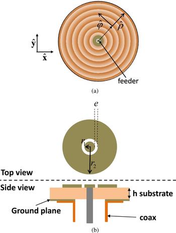
Figure 3 describes the feeding structure generating the cylindrical wave excitation. The feeder consists of a circular patch of radius r 2 with an annular slot of inner radius r 1. The slot is also described by its thickness e (Fig. 3(b)).

Fig. 3. Structure generating the cylindrical wave excitation. (a) Position of the feeder. (b) Structure of the feeder.
For a fixed substrate of permittivity εr and thickness h, the antenna adaptation is influenced by the parameters r 1, r 2, and e. The resonant frequency is mainly controlled using the outer radius r 2. On the other hand, the parameters r 1 and e have more influence on the level of the scattering parameter |S 11| at the resonant frequency.
Figure 4 represents the variations of the scattering parameter |S 11| in dB with respect to the frequency for different values of the outer radius r 2. The metasurface is printed on a substrate Rogers TMM6 of thickness 1.27 mm and relative permitivity 6. The curves were simulated using the software HFSS for the parameters (r 1;e) = (0.8;0.25) mm. It can be seen from the figure that the resonant frequency is shifted by varying the parameter r 2.

Fig. 4. Metasurface adaptation with respect to the outer radius r 2 for a substrate Rogers TMM6 of permittivity 6 and thickness 1.27 mm.
In Fig. 5 the variation of the parameter |S 11| in dB for different values of the inner radius r 1 is presented. It can be seen from the figure that the parameters mainly affects the level of the scattering parameter at the resonant frequency even though it produces a slight frequency shit. The latter has to be corrected by readjusting the outer radius r 2. A similar behavior is observed with the parameter e.
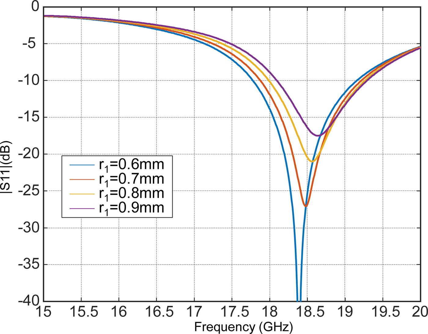
Fig. 5. Metasurface matching with respect to the inner radius r 1 for a substrate Rogers TMM6 of permittivity 6 and thickness 1.27 mm.
IV. NUMERICAL RESULTS
Following the design procedure developed in Sections II and III, two metasurface antennas able to radiate a broadside Rright-hand circularly polarized (RHCP) beam at 12.25 GHz and two independent beams at 20 GHz were designed.
The broadside RHCP antenna was designed for a substrate FR4 of thickness 1.6 mm and relative permittivity 4.4 with a diameter of 13λ. The objective aperture field distribution was calculated with MATLAB using equations (10) and (12). Its representation in the cylindrical coordinates is given in Fig. 6. The corresponding local reactance tensor components  $X_{11}^{loc} ({\bf {\rho} ^{\prime}})$ and
  $X_{12}^{loc} ({\bf {\rho} ^{\prime}})$ are illustrated in Fig. 7.

Fig. 6. Aperture field distribution for the broadside RHCP radiation pattern. (a)  $\left\vert {E_\rho ^{obj}} \right\vert $; (b)
  $\arg (E_\rho ^{obj} )$; (c)
  $\left\vert {E_\phi ^{obj}} \right\vert $; (d)
  $\arg (E_\phi ^{obj} )$.

Fig. 7. Variations of the reactance tensor components for a broadside RHCP metasurface. (a)  $X_{11}^{loc} ({\bf {\rho} ^{\prime}})$ (Ω); (b)
  $X_{12}^{loc} ({\bf {\rho} ^{\prime}})$ (Ω).
Using an in-house MATLAB code based on the proposed procedure, the metasurface giving the objective aperture field distribution was generated. The metasurface was then imported in the simulation software ANSYS Designer in order to simulate the radiation pattern. Figure 8 represents the circular components of the simulated far-field radiation pattern for the ϕ = 0° cut-plane. The left-hand circularly polarized (LHCP) component is represented in red while the RHCP component is represented in blue. We can see from the figure that the metasurface radiates the desired RHCP beam at broadside with a cross-pol level of −30 dB.

Fig. 8. Far-field radiation pattern (normalized) in dB for the ϕ = 0° cut-plane. The RHCP component ERHCP is given in solid line while the LHCP component ELHCP is given in dashed lines.
As a second example, an antenna radiating the first beam at (θ 0, ϕ 0) = (30°, 0°) with linear polarization along the ϕ-axis and a second beam pointing at (θ 0, ϕ 0) = (45°, 135°) with RHCP has been considered.
The metasurface has a radius of 5λ and has been realized printing the conducting elements on a Rogers TMM6 substrate of thickness 1.27 mm and relative permittivity 6. The incident surface wave with a cylindrical wave front was generated using a feeder of parameters (r 1;r 2;e) = (0.8;3.5;0.25) mm and placed at the center of the metasurface.
Figure 8 represents the aperture field distribution (phase and amplitude) required to obtain the desired two beams radiation pattern in cylindrical coordinates. The aperture distribution has been calculated with MATLAB using equations (10) and (12).
The corresponding local reactance tensor components  $X_{11}^{loc} ({\bf {\rho} ^{\prime}})$ and
  $X_{12}^{loc} ({\bf {\rho} ^{\prime}})$ are illustrated in Fig. 9. As it can be seen from Fig. 10, the complexity of the aperture distribution needs a strict control of the phase and amplitude of the generated LW.

Fig. 9. Aperture field distribution of the two beams metasurface antenna [Reference Teniou, Roussel, Capet, Piau and Casaletti9]. (a)  $\left\vert {E_\rho ^{obj}} \right\vert $; (b)
  $\arg (E_\rho ^{obj} )$; (c)
  $\left\vert {E_\phi ^{obj}} \right\vert $; (d)
  $\arg (E_\phi ^{obj} )$.

Fig. 10. Variations of the reactance tensor components for a two beams metasurface [Reference Teniou, Roussel, Capet, Piau and Casaletti9]. (a)  $X_{11}^{loc} ({\bf {\rho} ^{\prime}})$ (Ω); (b)
  $X_{12}^{loc} ({\bf {\rho} ^{\prime}})$ (Ω).
A metasurface having the corresponding impedance values has been generated using our in-house MATLAB code and simulated on the software ANSYS Designer. The designed structure is represented in Fig. 11 and the corresponding far-field radiation patterns for the ϕ = 0° and ϕ = 135° cut-planes are given (in black) in Fig. 12. The simulated radiation pattern is compared with radiation given by the perfect continuous objective aperture field distribution (in blue) and with the free-space radiation resulting from the equivalent magnetic currents (in red).

Fig. 11. Metasurface structure on ANSYS Designer.

Fig. 12. Far field radiation pattern in dB. (a) ϕ = 0° cut-plane E phi. (b) ϕ = 0° cut-plane E theta. (c) ϕ = 135° cut-plane ELHCP. (d) ϕ = 135° cut-plane ERHCP.
As can be seen from Fig. 12, the far field radiated by the metasurface antenna corresponds to the objective multi-beam radiation pattern and is in close agreement with the theoretical results. As expected, we obtained the first beam with linear polarization along the ϕ axis, pointing at θ = 30°, ϕ = 0°, as well as a second beam, with RHCP pointing at θ = 45° and ϕ = 135°. The cross-polarization levels are equal to −16 dB for the first beam and −20 dB for the second.
V. EXPERIMENTAL RESULTS
In this section, a prototype metasurface antenna designed using the presented procedure is measured. The designed antenna radiates a RHCP broadside beam at an operating frequency of 12.25 GHz (Ku band). The manufactured circular metasurface of radius 13λ was printed on a substrate FR4 of thickness 1.6 mm and permittivity 4.4.
For the considered substrate, the antenna is matched with a feeder of parameters (r 1;r 2;e) = (0.8;3.5;0.25) mm. Figure 13 presents the measurement and simulation of the variation of the scattering parameter |S 11|(dB) with respect to the frequency. The manufactured antenna is represented in the inset of the figure. It can be seen from the figure that the antenna is matched at the desired frequency. In addition, a close agreement is found between the simulation and the measurement.
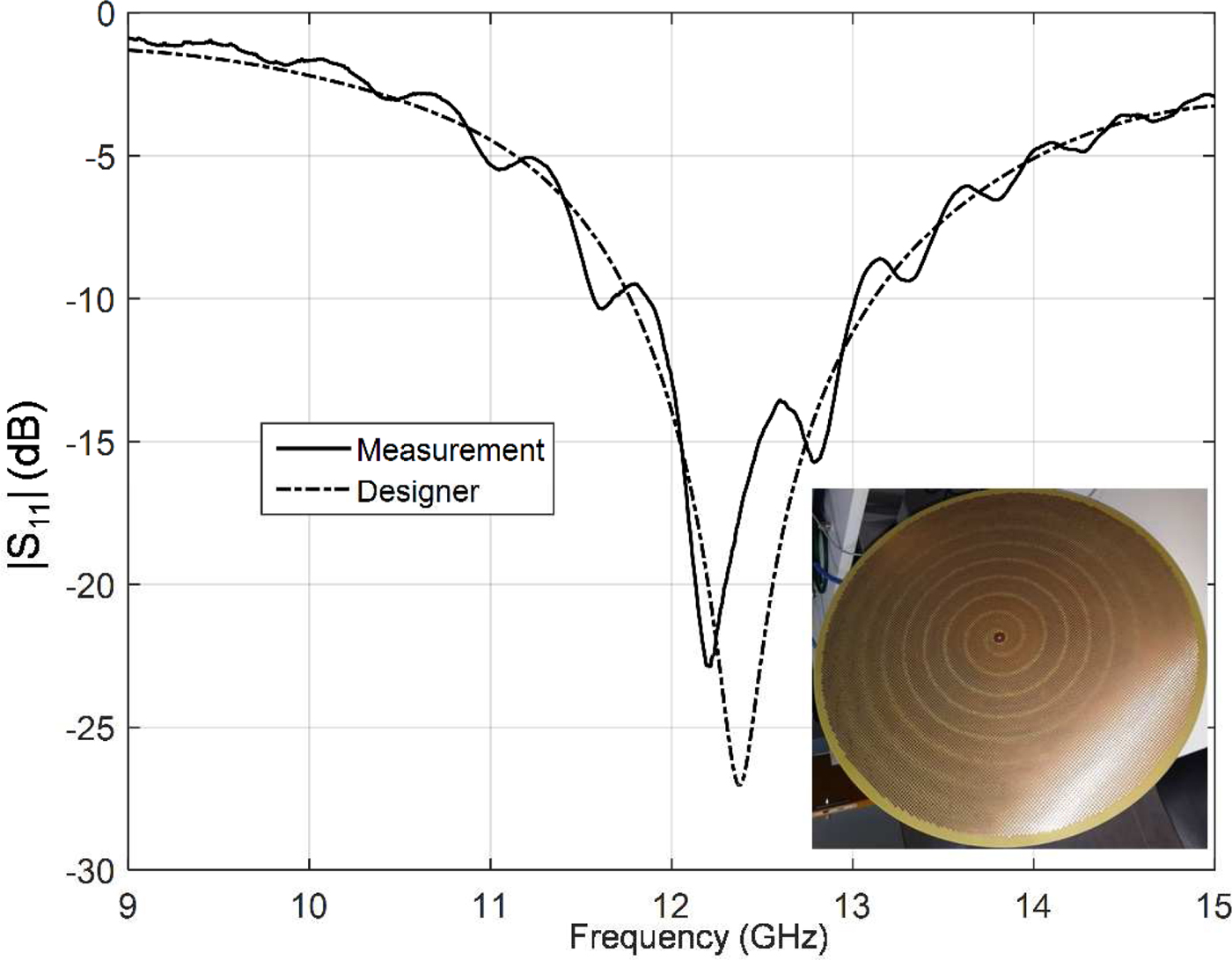
Fig. 13. Simulation and measurement of the scattering parameter |S 11|(dB) with respect to the frequency.
The far-field radiation pattern of the manufactured antenna was simulated in Designer and measured in the GeePs laboratory in France. The simulated radiation pattern (in red) and the measurement results (in black) for the ϕ = 0° cut-plan are presented in Fig. 14 at a working frequency of 12.25 GHz. The RHCP components are represented by solid lines while the LHCP components are presented in dashed lines. It can be seen from the figure that the desired RHCP beam is radiated at broadside with a measured cross-pol level of −20 dB. In addition, the measured side lobe level is −27 dB. A close agreement is obtained between the measurement and the simulation in the region of the principal lobe. The discrepancy outside of the lobes is probably due to the fact that the dielectric is assumed infinite in the simulations using Designer. There is a, therefore, discontinuity in the structure at the end of the metasurface. In addition, due to the complexity of the structure, the mesh quality is significantly limited by the computer performances.

Fig. 14. Simulation (in red) and measurement (in black) of the circular components of the far field radiation pattern (normalized) for the ϕ = 0° cut-plan. Solid lines represent RHCP components and dashed lines represents LHCP components. The working frequency is 12.25 GHz.
VI. CONCLUSION
In this paper, previous work on the generation of aperture field distribution using modulated tensorial metasurface is extended. The design procedure of the feeding structure and the antenna matching parameter are presented. The proposed method is validated with numerical simulations by comparison with theoretical radiation of perfect aperture field distribution. In addition, an antenna prototype is manufactured and measured giving good agreement with simulations results in term of scattering parameters and radiation pattern.
ACKNOWLEDGEMENT
We wish to thank the CNES (Centre National d'Etudes Spatiales) and Airbus Group Innovations for supporting this project.
 Mounir Teniou was born in Algiers, Algeria, in 1990. He received a bachelor of engineering from the National Preparatory School for Engineering Studies in Algiers, Algeria, and a Diploma in Electrical Engineering from the National polytechnic school of Algiers in 2010 and 2013, respectively. In 2014, he received a master degree in telecommunication systems from the University of Pierre et Marie Curie (UPMC) in Paris, France. He is currently a 3rd year Ph.D. student in L2E laboratory (Laboratoire d'Electronique et Electromangnetisme) of the UPMC. His Ph.D. thesis is founded by the French space Agency (Centre National d'Etudes Spatial) and Airbus Groups Innovations. His current research is about leaky-waves and metasurface antennas design.
 Helene Roussel received the Ph.D. degree from the University Pierre and Marie Curie (UPMC-Paris 6), France, in 1993. She is currently a Professor at the University Pierre and Marie Curie, since 2009, and her research is done at the Laboratoire d'Electronique et Electromagnétisme (L2E), UPMC, France. She is deputy director of this laboratory since January 2013. Her research interests include numerical methods and fast algorithms for electromagnetic scattering and radiation in complex media focusing on applications for metamaterials and on the analysis of wave propagation and scattering in random media for target detection and radar remote sensing.
 Mohammed Serhir received the Diplôme d'Ingénieur degree from Ecole Mohammadia d'Ingénieurs (EMI), Rabat, Morocco, and the Ph.D. degree in electronics from INSA de Rennes, France, in 2003 and 2007, respectively. Currently, he is working as an Associate Professor with CentraleSupélec, Gif-sur-Yvette, France. His research interests include antenna modeling and measurement in harmonic and time domains.
 Nicolas Capet graduated in electronic engineering and hyperfrequencies from the Ecole National d'Aviation Civile (ENAC), Toulouse, France, in 2007. He received in 2010 the Doctoral degree from Toulouse University in Electromagnetism and microwaves. Since 2010, he is working at CNES (Centre National d'Etude Spatiale, Toulouse) in the telecom division of the antenna department. In charge of antennas innovation for future applications, he was part of the project ownership for the antenna developments of ATHENA program and led multiple antenna studies for preparation of future missions. His current fields of interest are metamaterials applied to antennas (electromagnetic bandgap materials, reflectarrays, absorbers, metasurface antennas…), propagation of waves carrying Orbital Angular Momentum, Passive Intermodulation Products, innovative space telecommunication antennas, ground terminals for Satellite On The Move (SOTM) applications and antennas’ technological developments for competitiveness. Nicolas CAPET has just founded ANYWAVES and is developing a new generation of antennas dedicated to CubeSats and Drones.
 Gerard-Pascal Piau is a senior expert in Electromagnetic and Propagation. He received in 1986 a Ph.D. Thesis from the University of Lille in Laser and Interaction field. Since 1987, he is working at AIRBUS (ex Aerospatiale, and EADS) in microwave group, and specially for stealth and antenna application. He was in charge of multiple R&T and Ph.D. studies (development of new concept of radar absorbant material for the AIRBUS group, new measurement installations for antenna and radom, stealth software validation, antenna sitting on aeronautics platform, …). His current field of interest is now metamaterial applied to antenna and stealth concepts for industrial interests and applications.
 Massimiliano Casaletti was born in Siena, Italy, in 1975. He received the Laurea degree in telecommunications engineering and the Ph.D. degree in information engineering from the University of Siena, Siena, Italy, in 2003 and 2007, respectively. From September 2003 to October 2005, he was with the Research Center MOTHESIM, Les Plessis Robinson, Paris, France, under EU grant RTN-AMPER (RTN: Research Training Network, AMPER: Application of Multiparameter Polarimetry). He has been a Research Associate with the University of Siena from November 2006 until October 2010, and a Postdoctoral Researcher with the Institut d'Electronique et des Télécommunications de Rennes (IETR), University of Rennes 1, Rennes, France, from November 2010 to August 2013. He is currently an Associate Professor with the University Pierre-etMarie-Curie (UPMC), Paris, France. His research interests include numerical methods for electromagnetic (scattering, antennas, and microwave circuits), metasurface structures, field beam expansion methods, and electromagnetic band-gap structures.