


Introduction
Antarctica plays a major role in the Earth’s climate: the extent of the ice sheets and shelves affects the Earth’s radiation budget and ocean circulation. In addition, global-climate models show that the effects of global-climate changes, including those of possible greenhouse warming, are amplified in polar regions. The recent calving of large tabular icebergs off the Ross and Ronne— Filchner ice shelves (Reference Ferrigno and GouldFerrigno and Gould, 1987), as well as the rapid disappearance of the Wordie Ice Shelf (Reference Doake and VaughanDoake and Vaughan, 1991) on the Antarctic Peninsula, suggest that some ice shelves may be disintegrating rapidly. In spite of the possibly grave consequences of such ice-sheet disintegration, the current mass balance (the net gain or loss) of the Antarctic ice sheets is not known. Because of difficult logistic problems in Antarctica, field research has focused on only a few major ice streams and outlet glaciers. Yet, to understand the ice-sheet dynamics fully, we must carefully document all of the coastal changes associated with advance and retreat of ice shelves and outlet glaciers.
A critical parameter of ice sheets is their velocity field, which, together with ice thickness, allows the determination of discharge rates. Remote sensing, using moderate-resolution satellite images such as Landsat, permits glacier movement to be measured on sequential images covering the same area: the velocity of floating ice can be measured quickly and relatively inexpensively by tracking crevasse patterns on shelves and ice tongues. Landsat images are particularly useful because they provide synoptic views covering as much as 185 km2. Thus several fixed points in the scenes, needed for geometric corrections and coregistration of images, are likely to be found.
An extensive set of Landsat images covering Antarctica was acquired in the early to middle 1970s. Since 1984, new Landsat images of Antarctica’s coastal regions have been obtained largely through a program sponsored by an international consortium of nations belonging to the Scientific Committee on Antarctic Research (SCAR). These two sets of Landsat images, covering the same areas at different times, permit the measurement of glacier-feature movement. A period of nearly 20 years between acquisitions of some of the Landsat images makes them an invaluable resource.
Method
Selection of Landsat-image pairs
Many of the images of Antarctica that were acquired in the early to mid-1970s (Reference Southard and MacDonaldSouthard and MacDonald, 1974) are archived at the SCAR library of the U.S. Geological Survey in Reston, Virginia. They are Landsat 1, 2 and 3 multispectral scanner (MSS) images having a spatial resolution of about 80m per picture element (pixel). Reference Williams and FerrignoWilliams and Ferrigno (1988a) scrutinized all early images for ground portrayal, saturation (overexposure), and cloud cover, selected the best images for base-line studies to allow the detection of future changes, and published a catalog and map of the best images (Williams and Ferrigno, 1988b).
After a hiatus of many years, during which Landsat images of Antarctica were acquired only sporadically, renewed interest was sparked by modern digital image-processing techniques, and many new images were acquired (Reference Lucchitta, Bowell, Edwards, Eliason and FergusonLucchitta and others, 1987). A SCAR consortium pooled their resources to acquire recent MSS or Thematic Mapper (TM) images from Landsat 4 and 5, largely for purposes of mapping and detecting changes along the coastline. (TM images have a spatial resolution of about 30m/pixel.) The new acquisitions permit temporal measurements covering intervals of as much as 20 years. Our study focuses on such measurements.
After obtaining a plot showing the ground location of all newly acquired Landsat 4 and 5 images, we identified pairs of the old and new images covering the same area. We selected images that show outlet glaciers with floating termini (glacier tongues) and ice shelves with recognizable crevasse patterns. The crevasses, which may preserve their identity over many years, are used for the displacement measurements that lead to velocity determinations (Reference Lucchitta and FergusonLucchitta and Ferguson, 1986; Reference Orheim and LucchittaOrheim and Lucchitta, 1987; Reference Bindschadler and ScambosBindschadler and Scambos, 1991).
Examination of the image pairs showed that many glaciers do not have suitable floating tongues. Tongues on coastlines where ice shelves are narrow or absent tend to be short, perhaps due to vigorous current and wind regimes. Also, short tongues having distincitve crevasse patterns may break off in a time frame less than that between image acquisitions.
Large glacier tongues have two end members: (1) tongues whose crevasse patterns change rapidly and are difficult to trace after more than ten years between image acquisitions, and (2) tongues whose crevasse patterns remain virtually identical regardless of the number of years passed. Among the former are the Totten, Land, and Thwaites glacier tongues; among the latter are the Stancomb-Wills and Drygalski glacier tongues.
For our study, we obtained either computer-compatible tapes (CCTs) of MSS Landsat images, or, where tapes were nonexistent, the lowest generation transparency available for band 7 (near-infrared). These transparencies are third- and fourth-generation negatives, which have lost some image detail through the duplication process. We used only photographic products for TM images because of the high cost of CCTs. For TM images acquired before 1989 we obtained fourth-generation negatives and band 4 (near-infrared), and for images acquired after 1989 we used third-generation color negatives (only color photographic products are now available from the vending company). The quality of some of these images is poor, as they are not specially processed for the high reflectivity of snow and ice.
The transparencies were scanned at 50 μm to obtain a digital data set. The ground resolution of the scanned images varies, depending on their size. To obtain the ground resolution per pixel, the nominal Landsat-image height on the ground, in km, was scaled to the actual image height of the scanned pictures.
Coregistration and errors
For each matched image pair we designated three to six coregistration (control) points, preferably nunataks; where no nunataks were present, we chose distinctive coastline features, such as ice walls, that are stationary at the resolution of the images. For best results, the points should be as widely scattered across the images as possible; preferably, some are along the coastline and some on islands that occur along or seaward from the glacier tongues or ice shelves.
We generally registered Landsat 1, 2 and 3 images to Landsat 4 and 5 images, because the latter have more stable internal geometry and higher resolution than the earlier images. Reference Borgeson, Batson and KiefferBorgeson and others (1985) found that Landsat 5 images are accurate to about 0.4 pixels, meeting national Horizontal Map Accuracy standards for scales of 1:100 000 and smaller, and that Landsat 4 images are accurate to 0.8 pixel levels. Reference Welch, Jordan and EhlersWelch and others (1985) reported that Landsat 4 and 5 images meet accuracy standards for maps of 1 : 50 000 scale or smaller and are well suited to maps of 1 : 100 000 scale.
As our TM color images have been rephotographed at least once, with possible distortion, we performed our own accuracy test by comparing the geometric fidelity of a TM third-generation photographic print (Space Oblique Mercator projection) with the Mount Joyce quadrangle in north Victoria Land (scale 1:250 000; Lambert Conformai Conic projection). Despite the difference in projections, we found that our TM image was accurate to within 0.5% to 1% of the scale of a paper contour map of the quadrangle, and generally accurate to within less than 0.5% of the scale of a paper digital Landsat image mosaic of the quadrangle. The lesser accuracy on the contour map, which portrays features poorly, may be due to the difficulty in identifying common points on map and image. In addition, paper is not a stable medium. A 0.5% error over a distance of 10 km on the ground, a common distance found in our measurements, is only 50 μm on the image (at 1:1000000 scale), which is the size of one pixel. Thus, the error in scale should not severely affect our results. More precise scale-error investigations are in progress, using geodetic ground-control points tied to individual pixels in the TM image.
More problematic are internal scale distortions in the Landsat 1, 2 and 3 images due to roll, pitch, and yaw of the spacecraft. Coregistration with Landsat 4 and 5 images will reduce these errors, but for some of our pairs no such images were available. For the registration, we used a first-order polynomial involving rotation and translation of a rigid image. The residual errors for our fixed points remaining after coregistration are generally at the 2 pixel to sub-pixel level.
We again performed some first-order accuracy tests. We chose the Landsat image pair covering the Stancomb-Wills Glacier tongue, and we digitally coregistered the coastline and an island point 100 km from the coasdine beside the glacier tongue. The residual error for all points was 2 pixels or less. However, when we created a worst-case scenario and coregistered only the straight coastline but not the island point (Table 1), this point misregis-tered by as much as 26 pixels, or 1.3 km on the ground at the 1:1 000 000 scale of the image. Over a distance of 10 km the error would be 13%, and it would increase accordingly over shorter distances. Thus, if no coregistration points can be found near the sides of glacier tongues, and if Landsat 1, 2 and 3 images are used, measured displacements and resulting velocities can be unreliable for short distances. For larger distances (for instance, about 10 km) the possible error would decrease, but it could still be as much as 10% to 15%. However, for most of our images, coregistration points exist along the sides of
Table I. Error test. Stancomb-Wills Glacier Tongue (scale 1 : 1000 000) from Landsat 1 MSS 1579–0827, 22 February 1974 and Landsat 5 TM 50702–08511, 1 February 1986

ice tongues and errors are much less. For these images, the common maximum coregistration error of 2 pixels would be only 100m on the ground (at 1:1 000000 scale), or 1% over 10 km. Therefore, for all measurements involving Landsat 1, 2 and 3 images, our results should be good if the distances measured are large and if coregistration points exist around the glacier-tongue sides. For all Landsat 4 and 5 images the measurements should be very good, even if the distances are short and no such coregistration points exist.
Crevasse-pattern displacement measurements
We use an interactive display technique, developed for coregistration of planetary image maps, to measure the displacement of distinctive crevasse patterns on sequential images. The coregistered images, having identical line and sample numbers for the control points, are both displayed on a color raster screen, one image in the red and the other in the green image plane. Features that have moved between acquisition dates will appear as tones of green or red. Then, one of the images is moved until a chosen crevasse pattern is superposed exactly, resulting in a yellow tone for the coregistered feature. For each image, the offset line and sample numbers for each matched point are recorded. For large glacier tongues, we typically obtain 50 to 100 measurement pairs, but we may obtain fewer points if glaciers are small, crevasse patterns are indistinct, or image overlap is minimal. A computer program calculates the distance between the displaced points, which is the distance that the crevasse patterns have moved in the time between the two image acquisitions. Another computer program plots the displacement vectors onto the later Landsat image, which generally has better geometric fidelity than the earlier one. From the total distance traveled and the elapsed time, the average velocity (km a−1) is established for each point.
To obtain an idea of the distribution of velocities over the lengths of the glacier tongues, we also measured the distance from each point to an arbitrary baseline near the grounding line of the glacier (the boundary between the floating part of the glacier and the part supported by bedrock). This baseline may fall on the grounding line, but where the grounding line is irregular or at angles to the direction of movement, we drew the baseline approximately perpendicular to this direction. Because the velocity field may also vary across the glacier tongue, we subdivided the tongues into several longitudinal paths, each covering trains of distinct crevasse patterns. Paths are generally bordered by straight lines (by curved lines where glacier tongues are bent). We digitized the borders and projected them onto the images. Each measured point was then paired with its distance to the base line along the path of the nearest border. The results are shown in tables and graphs that give the distance from the base line versus the velocity for all points in each field. Our current software does not eliminate measuring errors, but we are now developing a routine that will statistically discount obvious stray points.
Results
So far we have investigated the Drygalski, Land, Thwaites, Berg, Stancomb-Wills, and Kaya glacier tongues ( Fig. 1). In addition, we have looked at several unnamed tongues on the Riiser-Larsen Peninsula ice shelf north of Kaya Glacier. Average velocities range from near 0.2 km a−1 for tongues on shelves to more than 2.5 km a−1 for the very fast moving Thwaites Glacier that discharges ice from the West Antarctic Ice Sheet into Amundsen Sea. All glacier tongues appear to increase in velocity as a function of distance from the grounding line.

Fig. 1. Antarctica: locations of investigated glacier tongues and outlines of Landsat images.

Fig. 2. Drygalski Ice Tongue. Displacement vectors and distances during 15.9year period. Landsat 4 TM image 42344-20284, 15 December 1988.
At this stage of our research we have not attempted to place our data into the glaciological context of the region; we invite comments concerning this context from interested researchers. However, we noted that the measured West Antarctic ice tongues are, in general, moving faster than those measured in East Antarctica. Causes may include differences in accumulation rates of snow and the marine bases of the West Antarctic ice sheet. Nevertheless, this observation may be significant in light of the hypothesized possible disintegration of the West Antarctic ice sheet (Reference MercerMercer, 1978) and the accompanying sea-level rise.
The results of our investigation are given in detail below. We show images of the investigated glacier tongues and their velocity vectors. The vector lines are plotted on the later image; therefore the measurement points are located at the outward end of the lines. Velocity measurements on individual ice tongues are shown in graphs plotting the average annual velocity against the distance from the baseline. The straight lines on the graphs are linear regression lines.
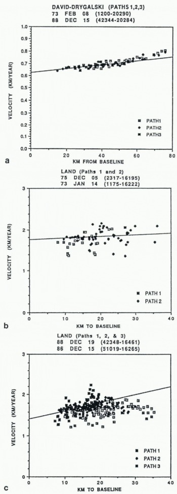
Fig. 3. Average annual velocity plotted against distance to baseline, a) Drygalski Ice Tongue, 15.9year interval, b) Tongue of the Land Glaner, 3.9year interval, c) Tongue of the Land Glacier, 2.0-year interval.
Table II. Average ice-tongue velocities

David-Drygalski Glacier Tongue
David Glacier traverses the Prince Albert Mountains and drains approximately 224000 km2 of ice from the Antarctic Plateau (Reference McIntyreMcIntyre, 1984; McIntyre, in Reference SwithinbankSwithinbank, 1988) into the Ross Sea. Its seaward extension, called the Drygalski Ice Tongue, extends for about 80 km beyond the grounding line and is approximately 22 km wide at the 500 m sounding (Reference ChinnChinn, 1980).
Where the ice tongue extends into the sea it encounters no adjacent land masses or islands to influence its direction or speed of flow ( Fig. 2).
Where the tongue begins to float, distinctive crevasse patterns appear and remain identifiable even throughout the nearly 16 year time span of our two Landsat images (Table 2). Almost the entire tongue moved as a coherent mass during this time interval. As a result we were able unambiguously to recognize and track 73 points.
Figure 3a shows a positive linear trend along the axial direction of flow, with very little scatter in the velocities. The graph also shows a small increase in velocity as the tongue moves seaward, but little variation in velocity across the tongue (perpendicular to the flow direction). This observation is confirmed by the similar velocities measured in the three axial fields into which we subdivided the tongue (Figs 2 and 3a). Our average velocity for the entire ice tongue of 0.70 km a−1 is close to Holdworth’s (1985) figure of about 0.75 km a−1. Indeed, his measurement, taken 50 km from the coastline, agrees exactly with our measurement at this distance.
Land Glacier
Land Glacier with its associated tongue is one of three fast-moving glaciers we examined that drain the West Antarctic ice sheet. Located on Ruppcrt Coast, it drains part of Marie Byrd Land and discharges in the Pacific Ocean sector. It extends for approximately 40 km from its grounding line and ranges in width from 15 km at its grounding line to about 25 km near its outer margin.
Two image pairs cover this glacier (Figs 4 and 5). Each pair spans a period of only a few years, but the two pairs are separated by an 11 year hiatus (Table 2). Unfortunately, the long time-gap between pairs, coupled with the rapid disintegration of the glacier tongue, precludes tracking crevasse patterns between the two image pairs.
The tongue of the Land Glacier emerges from accumulation areas that are more restricted on the east side (Path 1) of the glacier than on its west side (Path 3) ( Fig. 5). The glacier tongue is also pervasively fractured by crevasses, resulting in an unstable, incoherent mass. Around its periphery it breaks up into small polygonal segments.
Both of these observations are reflected in our graphs. Figure 3c shows that the velocities are generally lower on the east side of the ice tongue (Path 1), reflecting the smaller accumulation area. Average velocities are higher in the middle and on the west side (Paths 2 and 3). Also, velocity values, even though increasing slightly toward the distal end of the tongue, are highly scattered on the plot, indicating diflering velocities at the same distance from the baseline. The variation in velocities can be attributed to the breakup of the tongue where pieces of ice independently rotate and disintegrate and move at different velocities near the margins. This breakup also results in intense fragmentation close to the grounding line. Detailed examination of Figure 3c shows that more of the scatter is in the velocity values in Paths 1 and 3 (which include the edges of the glacier) and less in the central path, as one would expect.
The average annual velocity for the earlier image pair,1.80 km a−1, agrees reasonably well with the average annual velocity of the later image pair, 1.69 km a−1 (Table 2). The discrepancy may be real, reflecting a reduction in glacier velocity, but it is more likely caused by errors within the images or by errors associated with measurements. The earlier Landsat 1 and 2 MSS images have internal distortions which can lead to unreliable results. The later Landsat 4 and 5 images have minimal internal and scale distortions. Also, the TM images of the second set provided a threefold increase in resolution, enabling us to select a more accurate data set. Therefore, we consider the 1.69 km a−1 average velocity to be the more reliable of the two values.

Fig. 4. Land Glacier and its tongue. Displacement vectors and distances during 3.9year period. Landsat 2 MSS image 2317–16195, 5 December 1975.

Fig. 5. Land Glacier and its tongue. Displacement vectors and distances during 2.0year period. Landsat 4 TM image 42348–16461, 19 December 1988.
Comparison of the earlier and later image sets also shows that the glacier tongue retained its approximate dimensions. However, none of the crevasse patterns from the earlier images could be identified on the later ones, confirming the intense breakup discussed earlier. At least half of the tongue in the later images appears to be composed of ice discharged more recently from the ice sheet.
Thwaites Glacier Tongue
Thwaites Glacier drains a 121 000 km2 area of the West Antarctic ice sheet (Reference McIntyreMclntyre, 1984; Mclntyre, in Swithinbank, 1988) and flows into Amundsen Sea off the Walgreen Coast. It is the fastest flowing of the glaciers we measured in West Antarctica. Average annual velocities for our two data sets are 2.62 km a−1 and 2.84 km a−1, respectively (Table 2). These values correspond well with estimates of “over 2 km a−1” from Allen quoted in Reference Thomas, Sanderson and RoseThomas and others (1979). The images in each set (Table 2) and the ability to identify and track features between the two sets give continuous velocity data over a twelve-year time span (Fig. 6a and b). These data sets and our results are discussed in more detail in the companion paper by Ferrigno and others (this volume).
Berg ice stream
The ice stream and its accompanying glacier tongue ( Fig. 7) flow westward from the south end of the English Coast into the restricted waters of Stange Sound, Bellingshausen Sea. The glacier tongue is about 10 km wide at the grounding line and approximately 20 km long. It is arcuate, bending slightly to the west, probably due to an island that appears to divert the glacier tongue in that direction.
At 0.98 km a−1 (Table 2), the Berg Ice Stream is the slowest glacier tongue that we measured in the West Antarctica region. This velocity, even though fast by East Antarctica standards, appears to be in agreement with the small size of the glacier and its probable restricted accumulation area. The small size and short time span between images also result in a very small data set. The scattered velocity values (Fig. 6c) are to some extent an artifact of the fine scale in velocity increments on the vertical axis of the graph.
Stancomb-Wills Glacier Tongue
The Stancomb-Wills Glacier Tongue ( Fig. 8) dissects the northern part of the Brunt Ice Shelf and drains the area to the north and south of Heimenfrontfjella in Dronning Maud Land. It extends more than 200 km from the grounding line. Reference ThomasThomas (1973) established that the ice front moved about 1.5 km a−1 in the late 1960s.
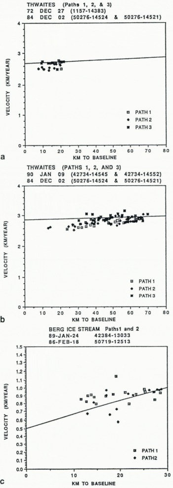
Fig. 6. Average annual velocity plotted against distance to baseline, a) Thwaites Glacier Tongue, 11.9year interval, b) Thwaites Glacier Tongue, 5.1year interval, c) Berg Ice Stream and its tongue, 2.9-year interval.

Fig. 7. Berg Ice Stream and its tongue. Displacement vectors and distances during 2.9year period. Landsat 5 TM image 50719–12513, 18 February 1986.
Beyond the grounding line, where the glacier begins to float, the tongue becomes intensely crevassed. Distinctive crevasse patterns are arranged along longitudinal tracks reminiscent of flowlines. The crevasse patterns are remarkably well preserved over the 12 year time span between image acquisitions, suggesting that the tongue moved as a coherent mass. The south side of the glacier tongue is fractured into several rotated icebergs 20 to 30 km wide and trapped in “thin shelf ice” (Thomas, 1973). On the north side, the glacier tongue appears partly confined by thick shelf ice and by Lyddan Island, even though some distance from the shore a narrow wedge of “thin ice shelf” separates the tongue from the main shelf.
Figure 9a shows that the glacier tongue increases in velocity from about 1 km a−1 near the grounding line to 1.2 km a−1 100 km from this line; it is exceptionally fast for an East Antarctic glacier tongue. The graph also shows the pinned side of the glacier (north side) moved most slowly, the side bordered by “thin shelf ice” and icebergs (south side) moved faster, and the middle of the glacier moved fastest.
Because the crevasse patterns are well developed and keep their identity with time, we used three different methods to calculate the velocities. Data were collected by hand measurements on the images, by automatic feature tracking (software developed by R. Kwok, Jet Propulsion Laboratory), and by our interactive digital process. The results from all three data sets agree extremely well, but only the last-men tior-ed is shown in this report.
Thomas (1973) obtained a velocity of 1.3km a−1 for a point on the north side of the ice tongue. We could not locate this point precisely, but it appears to be approximately 150 km from the grounding line, outside the area of our images. If so, our measurements projected to this point agree well with Thomas’s data.
Kaya Glacier and Riiser-Larsen Peninsula Ice Shelf
The two image sets that cover this area contain four glacier tongues, designated Α-D in Figures 10–12. Located on the eastern side of the Riiser-Larsen Peninsula along Prince Harald Coast in northeastern Dronning Maud Land, these tongues drain into Lützow-Holm Bay in the Indian Ocean sector.

Fig. 8. Stancomb-Wills Glacier Tongue. Displacement vectors and distances during 11.9year period. Landsat ΤM image 50702–08511, 1 February 1986.
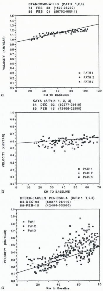
Fig. 9. Average annual velocity plotleed against distance lo baseline, a) Stancomb-Wills Glacier Tongue, 11.9year interval, b) Kaya Glacier and its tongue, 4.2year interval, c) Tongue Β on Riiser-Larsen Peninsula ice shelf, 4.2year interval.

Fig. 10. Kaya Glacier (bottom) and tongue Β (top) on Riiser-Larsen Peninsula ice shelf. Displacement vectors and distances during 4.2year period. Landsat 4 MSS image 42406–05500, 15 February 1989.

Fig. 11. Ice tongues B, C and D (bottom to top) on Riiser-Larsen Peninsula ice shelf. Displacement vectors and distances during 15.3year period. Landsat 4 MSS image 42406–05500,15 February 1989.
The tongue of Kaya Glacier (bottom, Fig. 10), extends approximately 65 km into the bay and is about 10 km wide and relatively coherent along its entire length. Its crevasse pattern is well defined. The average annual velocity for the tongue is 0.59 km a−1 (Table 2). As the tongue leaves the grounding line it bends slightly toward the east, perhaps due to drag from a small peninsula that juts into the bay and impedes the flow ( Fig. 10). The graph (Fig. 9b) shows that the glacier tongue moved most slowly on this side. The apparent scatter on this and all subsequent plots is to some extent the result of the fine velocity scale on the vertical axes of the graphs.
Tongue Β is the only one that occurs in both image sets. As a result we have more than 470 measurement points spanning a 15 year interval. About 65 km long and 10 to 40 km wide, it is by far the largest tongue on these images, with an average annual velocity of 0.42 km a−1 (Table 2). This tongue is very coherent for almost its entire length (Figs 10 and 11), but it begins to break up at the outer limits on its east side (Path 1). The breakup may be responsible for the scatter and increased velocities near the distal points of this path (Figs 9c and 12a). Path 3 shows clusters of low-velocity data points about 70 km from the baseline (Figs 9c and 12a). The low velocities, probably caused by small offshore island that impeded the flow, lower the average annual velocities recorded for this tongue in Table 2. We compared the average annual velocities of Path 3 obtained from both image pairs. The velocities differ by only 0.003 km a−1. The closeness of the results suggests a steady flow rate over the 15 year period of our images, thereby also confirming the accuracy of our measurements.
Effects of island masses hindering flow rates are also apparent in the velocities measured on glacier tongue C. At an average annual velocity of 0.12km (Table 2), this small tongue has moved the most slowly of all we measured. The reasons are probably the small accumulation area on the point of the peninsula and the presence of several small islands just offshore, directly impeding tongue movement ( Fig. 11). The separation of the flow into two parts is clearly evident on the velocity graph (Fig. 12b).
Tongue D, near the north edge of the image ( Fig. 11), is only partially shown in our images, so that measurements could not be made over its entire extent. Figure 12c shows some very low velocities near the base in a separate cluster of Path 1 (Fig. 11 ), due to a land projection jutting into the tongue. Because they lower the average velocity calculated for this tongue, the value of 0.38 km a−1 (Table 2) is probably too low.
Conclusion
Our studies show that it is feasible to obtain velocity measurements on the tongues of outlet glaciers of Antarctica from satellite images with an accuracy sufficient to monitor future changes. However, this accuracy requires future images of the quality of Landsat 4 and 5. We are now obtaining many additional image pairs for our measurements. Our plan is to inventory velocities of all outlet glaciers and ice shelves around the Antarctic periphery that have suitable crevasse patterns. We hope to obtain a data base that will not only be suitable for detecting future velocity changes but will also help mass-balance studies based on glacier-tongue thickness values derived from radio-echo sounding or future satellite-based laser altimeters. Thus, our studies will eventually help to monitor the effects of climate change in Antarctica.

Fig. 12. Average annual velocity plotted against distance to baseline; 15.3year interval; Riiser-Larsen Peninsula ice shelf, a) Ice tongue B. b) Ice tongue C. c) Ice tongue D.
Acknowlegements
We are grateful for helpful reviews by P.A. Davis, R.S. Williams, Jr, and two anonymous reviewers. The research was funded by NASA’s Polar Oceans and Ice Sheets Program and the U.S. Geological Survey.


