


In this article, we examine whether the policy in Britain is shaped by public preferences. We examine two accounts by which policy responsiveness could be achieved. “Policy accommodation” suggests that office-seeking governments respond directly to changes in preferences by changing policy. “Electoral turnover”, on the other hand, suggests that policy responds indirectly. Parties pursue policies consistent with their ideology. The public’s preferences respond to policy “thermostatically”, moving right as policy moves left and left as it moves right (Wlezien Reference Wlezien1995). These movements produce changes in vote intentions and, ultimately, a turnover of power from one “side” to the other. This process, however, may only operate after a considerable time lag if the public initially lacks faith in the competence of the opposition.
There are two sets of reasons why we should be concerned with whether the policy is responsive to public opinion. First, from a strictly positive point of view, we want to know to what degree government policy is constrained by public opinion. To what degree are policymakers forced to react to changes in public opinion and to what degree are they able to act independently of it? Second, from a normative point of view, we are interested in how “well” democracy is functioning – do governments act in a way that is representative of the public? Of course, there are many different conceptions of democracy, some of which do not require the congruence of public opinion and policy in a substantive sense.Footnote 1 Nevertheless, the basic meaning of democracy is that the “people rule”, and this is often interpreted to mean that the people should have control of the broad direction of policy (May Reference McGann1978; Rehfeld Reference Rehfeld2009; Petitt Reference Petitt2010). As Andrew Rehfeld puts it, “… the presumption of democracy is that there be a close correspondence between the laws of a nation and the preferences of citizens who are ruled by them” (Reference Rehfeld2009, 214).
However, when we consider representative democracy, it is not immediately obvious how responsive policy should be to public opinion, especially if we embrace a trustee conception of representation. If we think that the appropriate form of representation is a delegate model – the government ought to follow the instructions of the people – and we apply this to the government as a whole as opposed to individual representatives, then we should expect government policy to follow public opinion.Footnote 2 Of course, it is still necessary to interpret what the people’s “instructions” are.Footnote 3 Even in this case, we might expect the government to follow the will of the people in broad terms rather than in terms of specific policies. Following Christiano (Reference Clarke, Stewart, Sanders and Whiteley1996, 215–217), we might expect the government to be a delegate in terms of ends, while being a trustee in terms of means.
However, if we endorse a trustee model of representation – representatives are expected to use their judgement to advance the interests of the people to the best of their ability – then a considerable amount of slippage between public opinion and policy may be completely acceptable in a democracy. It is still possible that trusteeship will produce a high degree of responsiveness. If the people choose trustees whose values and interests align closely with their own, they may choose policies that naturally track the preferences of the public (what Mansbridge Reference McDonald and Budge2003 terms “gyroscopic representation”). Similarly, trustee representation and popular control could be reconciled through deliberation and public reason, in what Pettit calls “interpretive representation”.Footnote 4 On the other hand, while trustees are expected to act in the interest of the public, they also may choose policies that differ from what the public wants. If the policies demanded by the public want are impossible or ill-advised (they do not achieve the ends the public wishes to achieve), then trustee representation will result in policies that diverge from what the public wants.Footnote 5
However, it is important not to take this argument too far. While trustee representation allows for some slippage between public opinion and policy, we should still be concerned if there is a complete disconnect. If democratic trusteeship allows the public to be completely disregarded, then there is a danger that it simply becomes a euphemism for benign despotism or paternalism. A trustee, according to Burke (Reference Burke2009), must make decisions in the interests of the people, and may not substitute their own interests in place of those of the people. When we observe government policy diverging from public opinion, we are faced with the question as to whether this is the legitimate use of trusteeship in the interests of the people, or whether the government is substituting its own interests for those of the people. Lack of policy responsiveness certainly does not prove that there has been a failure of democratic representation, but it does call for explanation and justification. As Rehfeld argues, “we must always justify and explain cases in which law deviates from citizen preferences, whereas no such prima facie justification is required in cases when law conforms to the preferences and wills of those it governs” (Reference Rehfeld2009, 214).
Thus, while responsiveness does not give us a simple measure of democratic representation, it can still provide a valuable test of it. We would argue that the responsiveness of aggregate public spending to public opinion is actually a more appropriate test than the responsiveness of particular policies or the budget allocations to particular departments. This is because it is a very general measure of policy that reflects broad visions of society, rather than specific policy expertise. If detailed public policies do not reflect public opinion, a government can always claim that it is acting as a trustee, using its superior technical knowledge to make informed decisions. It may even claim that what the public wants is impossible. However, it is clearly possible to have different levels of aggregate spending and taxes, as this varies greatly amongst countries.Footnote 6 Furthermore, there does not exist a technocratic consensus about what the appropriate size of government is; rather this appears to be a matter of values, and the type of society people prefer. If the government persistently ignores public opinion in such a general sense, we may well worry that it has exceeded its role as trustee and substituted its own values for those of the people.
In addition to the policy responsiveness we study, other forms of responsiveness may also be valuable in testing how representative government is. One example is attention responsiveness (Jennings and John Reference Jennings and Wlezien2009; Bertelli and John Reference Bertelli and John2013; John et al. Reference John, Bertelli, Jennings and Bevan2013; Bevan and Jennings Reference Bevan and Jennings2014). This considers the degree to which the policy priorities of governments (typically measured by the weight given to various policy areas in the Queen’s speech) corresponds to the policy priorities of the public (usually measured by the answer to the question of what is the most important problem facing the country). While policy responsiveness and attention responsiveness both deal with the allocation of a scare resource (money or time), they seem to behave quite differently (see Bevan and Jennings Reference Bevan and Jennings2014; Jennings and Wlezien Reference Jennings and John2015).Footnote 7 Nevertheless, if a government is representative of the people, we would expect it to pay attention to the issues that the people think are important, even if it does not necessarily allocate more money to these areas. If a government consistently ignores the issues the people think are important, we are surely entitled to ask whether the government is really representing the interests of the people.
While responsiveness may not provide us with a direct measure of democratic representation, it does provide a valuable of a test of it. If we do not observe responsiveness (whether in policy or attention), this may serve as a warning flag that demands explanation. This caveat aide, we examine the relationship between preferences and policy in Britain from 1945 to 2015 using macrolevel indicators and appropriate time series methods. In the next section, we introduce the left-right framework to summarise preferences and policy. In the next two sections, we conceptualise both these as time series (“the policy mood” and “nonmilitary government spending”) that respond to each other. We describe the time series models in some detail before examining the two steps in the “electoral turnover” mechanism (whether mood responds to policy and vote to mood). We then examine both the final stage in the electoral turnover mechanism (whether policy responds to the party) and the policy accommodation mechanism (whether policy responds to mood). We finally compare our findings with previous studies and then we draw conclusions about the impact of party ideology.
The left-right framework
Disagreements about goals are central to most accounts of representative democracy because they motivate parties and electorate alike (Downs Reference Downs1957). Parties pursue ideological goals subject to electoral considerations (Strøm Reference Strøm1990). The electorate wants governments both to produce policy that honours their values and govern with competence (Stimson et al. Reference Stimson, MacKuen and Erikson1995; Erikson et al. Reference Erikson, MacKuen and Stimson2002). Preferences and positions link parties with the electorate and provide the basis for effective communication (Scarbrough Reference Scarbrough1984).
There are a very large number of issues that people disagree about. If we are to understand the interaction between parties and the electorate we need to cut away inessential detail (Budge Reference Budge, McDonald and Ezrow2006). Accordingly, we assume that the interaction between parties and the electorate takes place along a single left-right dimension (Downs Reference Downs1957). The preferences that are of interest to us are those on which the parties have taken positions. “Left” means those preferences expressed or positions adopted by Labour. “Right” means those adopted by the Conservatives (Budge and Farlie Reference Budge1977).
Parties aim to attract voters. They take positions on a wide range of issues. Some are enduring. Some are transient. The “core” issues that divide the major parties relate to economics. Labour has generally supported “more” government activity, “more” collective action and “more” equality. The Conservatives have generally supported “less” (Blais et al. Reference Blais, Blake and Dion1993). Nevertheless, Labour and the Conservatives disagree on other issues relating to law and order, individual freedom, the environment and international affairs. As new issues emerged, the parties have adopted opposing positions, and these have acquired “left” or “right” polarities (Carmines and Stimson Reference Carmines and Stimson1989). It is usual, for example, to label support for shorter sentences, equal rights for gays, environment protection and international cooperation as “left-wing”. This enables analysts to use texts to summarise party positions using both economic and noneconomic positions. The MARPOR “RILE” scores, for example, provide evidence about how parties compete for office (Budge et al. Reference Budge2001; McDonald and Budge Reference Mansbridge2005).
There are doubts whether public preferences can be so simplified (Budge Reference Budge, McDonald and Ezrow2006). Fortunately, it is not necessary to resolve the vexing issue of the “real” structure of public preferences here (Stimson Reference Stimson2004). Our purpose is simply to summarise preferences in such a way as to understand the interaction between parties and the electorate. Accordingly, we focus on the core economic issues that represent the enduring differences between the parties relating to government intervention, collective action and economic equality (Heath et al. Reference Heath, Evans and Martin1994). This decision also simplifies the measurement of policy since it is difficult – if not impossible – to produce annual measures of policy that incorporate both economic and noneconomic issues using textual data.Footnote 8
Measuring macrolevel preferences: annual policy mood
If we are to analyse responsiveness we need a public preference time series (Erikson et al. Reference Erikson, MacKuen and Stimson2002). Microlevel theories provide us with good reasons for believing that we can use preferences across a wide range of issues to produce an annual indicator of public preferences. Many issues become “seemingly relate”’ and acquire “left-right” polarities (Carmines and Stimson Reference Carmines and Stimson1989). Since most people have low levels of political awareness, they absorb both “left” and “right” considerations (Zaller and Feldman Reference Zaller and Feldman1992). The typical individual is “ambivalent” about issues. Their responses to questions depend on their predispositions, the issues raised, precise wording and response options offered. Individual predispositions can be viewed as a running tally of “left” and “right” considerations across all issues. If we could aggregate preferences across both individuals and issues, this “double summation” would provide an indicator of the electorate’s aggregate (varying) left-right preferences or “policy mood” (Stimson Reference Stimson1999).
We cannot directly average aggregate responses across survey items. Each survey question has its own biases as a result of the issues that it engages, precise wording and response options provided (Zaller and Feldman Reference Zaller and Feldman1992). Each question has its own metric. Nevertheless, we can use a method – the dyads ratio algorithm – to find a common metric and then aggregate across issues (Stimson Reference Stimson1999). Before we outline this method, however, we describe the data at our disposal.
Data: the preferences database
Responses to a wide range of survey probes reflect left-right preferences. Variations in responses over time should, therefore, reflect the changing “policy mood” (Stimson Reference Stimson1999). The raw data to estimate mood are aggregate responses to controversial questions. They require people to choose between options, express “preferences”, adopt “positions” or take “sides” (Stokes Reference Stokes1963; Ellis and Stimson Reference Ellis and Stimson2012).
Since mood is inferred by observing changes between two time points, identical questions must be asked in at least two separate years to form “dyads” (Stimson Reference Stimson1999). Items that refer to particular parties or politicians are excluded from the database, since it is difficult to disentangle attitudes to these objects from preferences.Footnote 9 All the data are taken from nationally representative surveys. In total, the database contains 791 items and 5,363 separate readings of preferences.Footnote 10
Content
Our database consists of responses to many controversial issues on which the parties can be expected to take contrasting positions. Some 287 questions in 2,087 separate readings of preferences (39.7% of the total) relate to “core economic” domain, including government intervention, trade unions, public ownership, public spending, taxation, inequality and the trade-off between inflation and unemployment (see Table 1). Another 1,102 readings (21% of the total readings) relate to “social” issues. This domain includes crime and law and order, moral and social attitudes, individual rights, the family and abortion. The “other” category (around 40% of all readings) relate to diverse issues including immigration, international affairs, defence spending, nuclear weapons, Northern Ireland, Europe, national sentiment, the monarchy and left-right self-placement.
Table 1 Items topics for policy mood, 1945–2015
Note:
* Indicates used to estimate the policy mood.
If we were confident that public preferences – like party positions – were undimensional, we could estimate mood using all the available data. Since we are ignorant of the real structure, we estimate mood using only items relating to the “core economic” issues. Even after this self-imposed restriction, however, there here is more than sufficient data to reliably estimate annual mood.
Coding responses
Our focus here is on the “core” left-right issues. Responses are scored from high (most left or Labour) and to low (most right or Conservative) responses. It is straightforward to code these items since the parties have taken consistent (opposing) positions.Footnote 11 Assigning the “wrong” polarities to responses makes no difference to the estimates of mood – it simply results in negative factor loadings that alert us to a coding error (Stimson Reference Stimson1999).
All preferences are expressed as an index of preferences:
 $${\rm Index}\,{\rm of}\,{\rm preferences}\,{\equals}\,{{\sum_{i\,{\equals}\,1}^N {\rm Left}\,{\rm preferences}} \over {\sum_{i\,{\equals}\,1}^N {\rm Lef}{\rm t}{\plus}{\rm Right}\,{\rm preferences}}}{\rm }{\times}100$$
These indexes reflect then the balance of left-right preferences on controversial issues. They are fed into the dyads ratio algorithm in order to estimate mood.
Method: the dyads ratio algorithm
The raw index of preferences represents the percentage of all substantive responses that are “left”.Footnote 12 Each index is then expressed as a ratio at two time points (years).
 $$R_{{ij}} \,{\equals}\,{{x_{{t{\rm {\plus}}i}} } \over {x_{{t{\rm {\plus}}j}} }}$$
These dyads have an expected value of 1.0 and can be averaged to produce a rough estimate of underlying preferences (P t ). The algorithm calculates all the possible dyads for each series x tk iteratively and averages them:Footnote 13
 $$P_{t} \,{\equals}\,{{\sum_{k\,{\rm {\equals}\,1}}^N x_{{tk}} } \over N}$$
Since not all items are equally valid indicators of underlying preferences, each series is weighted by their estimated validity hi 2.
 $$P_{t} \,{\equals}\,{{\sum_{k{\rm \,{\equals}\,1}}^N h_{i}^{2} x_{{tk}} } \over {h^{2} N}}$$
Using ratios causes the original metric to be lost. This is reintroduced by a standardisation of the latent scale in terms of the validity-weighted means and standard deviations of the input items (Stimson Reference Stimson1999). The individual items are scored as per cent left over per cent left plus per cent right. The estimated mood, therefore, has the same interpretation; 50 is the neutral point. Values above 50 indicate net left preferences and those below 50 indicate net right preferences.
Estimates of the policy mood
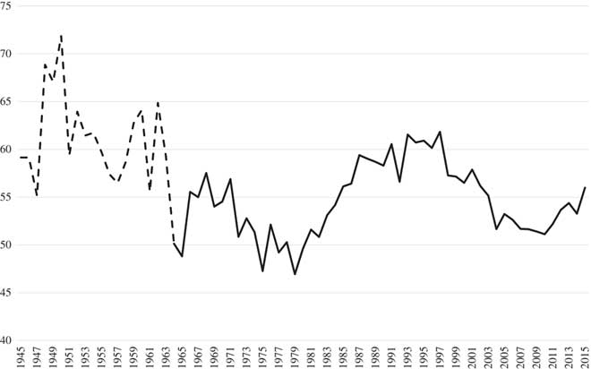
Figure 1 displays the estimated mood from 1945 to 2015. About 46% of all variance in observed preferences is common to this mood. The remaining variance – some 54% – is either specific to the particular issue domain or is item-specific; that is, a function of the specific wording and measurement error for each question (Erikson et al. Reference Erikson, MacKuen and Stimson2002, 203).

Figure 1 The policy mood, 1945–2015.
Averaging over many items reduces the noise induced by sampling errors (Stimson Reference Stimson1999).Footnote 14 In the early period from 1945 to 1964, when data are in shorter supply, the series zig-zags (shown by the broken line in Figure 1). In the later period, after 1964, the series is smoother (shown by the unbroken line). Nevertheless, the overall pattern is clear. The series starts off high (left) in the 1950s and then generally drifts down (right) until 1979.Footnote 15 From 1979 onwards the series tracks back up and to the left, peaking in the early 1990s. This pattern matches standard accounts of public opinion (Kavanagh Reference Kavanagh1988). From 1997 the series drifts down (right) under New Labour. It reaches its lowest point in 2010 when the Conservatives return to power in a coalition government. It then reverses itself under the coalition government between 2010 and 2015. Indeed, by 2015, the mood was as far left as it had been in 2004, the year before Labour won a third election victory.
Broadly speaking, these movements seem to be related to the electoral performance of the parties. This suggests that the mood series has a degree of face validity. In particular, three “turning point” elections were presaged by movements in the mood. The Conservative victory in 1979, New Labour’s landslide in 1997 and the Tories return to power – as the dominant party in the coalition in 2010 – all appear to reflect prior movements. Yet some election outcomes do not seem to be explicable given movements in the mood. The October 1974 and 1979 general elections, for example, produced a Labour victory on the one hand and a Conservative victory on the other, despite the similar levels of mood. Similarly, the 1992 and 1997 elections produced a Conservative victory and a Labour landslide, though the mood was at much the same level. Other factors – social change, party positions and assessments of party competence – must be taken into account.
In order to illustrate the content of mood, we briefly examine the factor loadings for individual items on the estimated mood series. Since there are 287 series, it is not possible to examine all the loadings. And, since the series vary in length, it would be misleading examine the loadings for all the individual series. Table 2 displays the loadings for the items that are entered into the database in at least 10 years and load at 0.5 or above.
Table 2 Item loadings of policy mood, 1945–2015
The items that load on mood relate to trade unions, welfare, tax and spending, and inequality. This is a consequence of our decision to include only the “core” issues. The same items would feature prominently in the equivalent table if we had estimated the mood using all the preferences data.Footnote 16 The mood estimated from this larger database, moreover, correlates highly with our mood measure (Pearson’s R=0.90). These observations do not resolve the issue of the dimensionality of preferences. They do reassure us that our decision to use only “core” items is not consequential. Averaging a large number of items produces a robust estimator of preferences.
Measuring annual macrolevel policy
In order to assess the interaction between governments and the electorate, it is necessary to develop a measure of government policy analogous to our measure of mood. “Policy” is a course of action or the principles adopted by the government. It is difficult to summarise because governments take lots of action make many statements of principle. They legislate, enter into treaties, make administrative decisions, tax and spend, and issue statements of intent. It is also difficult to summarise because it can be indicated by both words (intentions) and deeds (actions and policy delivery).
Nonmilitary government spending
Spending is a particularly appropriate indicator of delivered policy. It provides a numeraire that gets to the heart of the choice between “more” or “less” (Blais et al. Reference Blais, Blake and Dion1996, 43; Soroka et al. Reference Soroka, Wlezien and McLean2006). The key indicator of total managed expenditure (TME), for example, summarises government activity in an annual time series. This includes Departmental Expenditure Limits that have been allocated to Departments and Annually Managed Expenditure that is not controlled by government departments.Footnote 17
The parties’ preferences about spending reflect their ideologies. Labour governments prefer “more” spending on welfare, health and transport. Conservative governments prefer “less”. In some domains, however, these preferences are reversed. The most significant case is defence spending. This fluctuated between a high of 9.8% of gross domestic product (GDP) in 1953 to a low of 2% in 2015.Footnote 18 In general, Conservatives prefer more and Labour prefers less spending on defence. Military spending, moreover, is influenced by perceptions of threat and is less responsive to domestic politics. In order to provide a more accurate indicator of domestic policy, we subtract defence as a percentage of GDP spending from TME to produce nonmilitary government expenditure (NMGE).
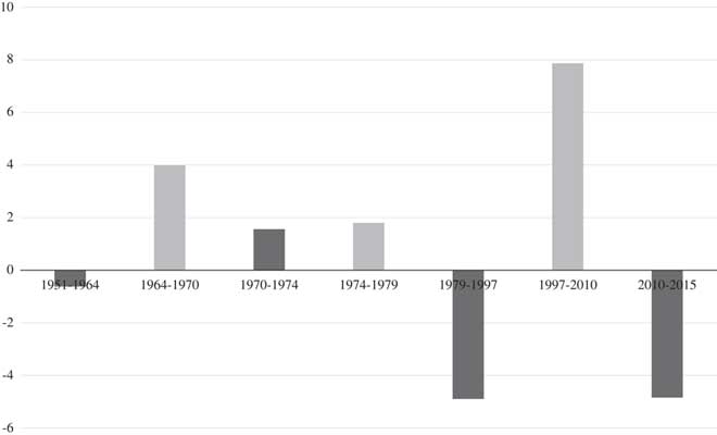
Figure 2 displays the NMGE series from 1950 through to 2015.Footnote 19 This provides evidence of year on year variation but says little about the impact of party control of government over policy. Figure 3 displays changes in NMGE under governments from 1951 to 2015. Dark blocs indicate Conservative governments; lighter blocs indicate Labour. This tells a fascinating story. All Conservative governments, with the single exception of Heath (1970–1974), have reduced NMGE.Footnote 20 All Labour governments have increased it. Our characterisation of elections as a choice between “more” with Labour and “less” with the Conservatives has a degree of face validity.
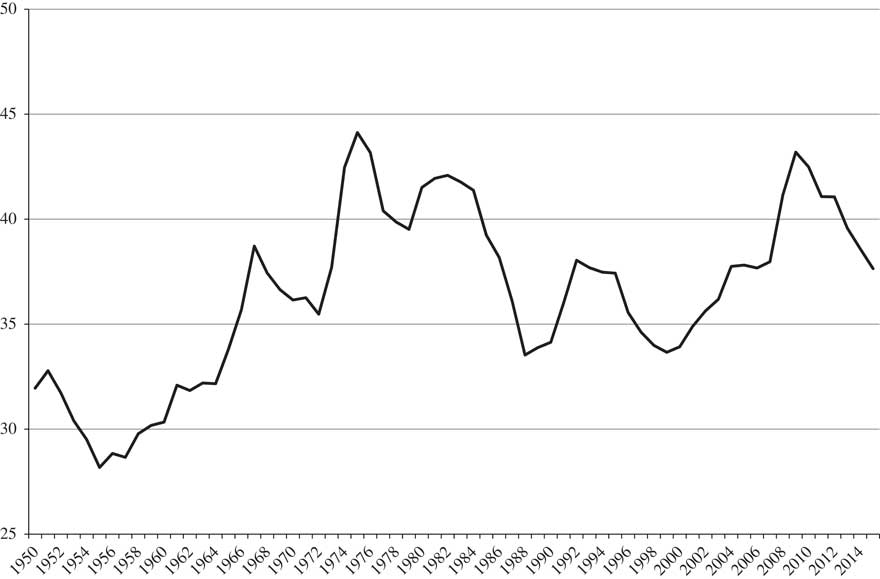
Figure 2 Nonmilitary government spending, 1948–2013.
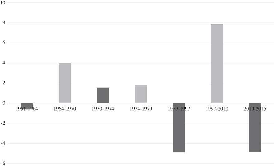
Figure 3 Changes in nonmilitary government expenditure by government, 1951–2015.
Average direct taxation
The electorate is collectively ambivalent about the government policy activity. They prefer “more” public services. They also prefer “less” bureaucracy and taxation. They also worry about the impact of welfare on individual incentives (Zaller and Feldman Reference Zaller and Feldman1992). Since it is difficult to produce time series indicators of bureaucracy and incentives, we focus on taxation.Footnote 21 Specifically, we incorporate a measure of the average direct tax (income tax plus national insurance) paid by male workers on median incomes (see Figure 4).Footnote 22 This measure does not, of course, cover all taxes but reflects public debates in Britain, which have centred on direct taxation.Footnote 23
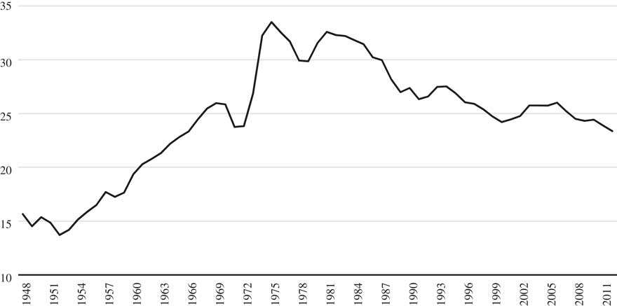
Figure 4 Average direct tax levels (1949–2012).
Methodology
When we inspect the graphs for mood, vote intentions and domestic spending, it is clear that these variables are not stationary. That is to say, they do not oscillate around a single mean, but instead the mean moves over time. Formal stationarity tests confirm this.Footnote 24 Nonstationarity creates problems when analysing time series, in particular the problem of spurious regression (Enders Reference Enders2004). It is quite likely that two nonstationary variables will correlate significantly, even if they are completely unrelated. We need to ensure that our results are not simply the result of such spurious correlation.
One approach to the problem of nonstationarity is to take the first difference of the data (or further differences if necessary), so we have a stationary time series. This deals with nonstationarity but only allows us to draw inferences about the short-term dynamics of the relationship between the variables. An alternative approach is to use the error correction model approach of the type:
 $$\Delta {\rm Y}_{{\rm t}} \,{\equals}\,{{\rm b}_{0}}{\plus}{{\rm b}_{1}}\,\Delta {\rm X}_{{\rm t}} {\plus}{\rm a}\left( {{\rm Y}_{{{\rm t}{\minus}1}} -{{\rm g}_{0}}-{{\rm g}_{1}}\,{\rm X}_{{{\rm t}{\minus}1}} } \right)$$
This also allows us to model the long-term relationships between the variables. It assumes that there is a long-term equilibrium relationship between the variables, and that the further out of equilibrium we are the larger the adjustment (the parameter a represents the speed of this adjustment). However, error correction models are only appropriate with nonstationary data if the variables are cointegrated (Engle and Granger Reference Engle and Granger1987). Roughly speaking, this means that the variables move up and down in parallel, and the relationship remains approximately the same over the whole time period.Footnote 25 If the variables are not cointegrated, we again face the problem of spurious regression.
We use the error correction model whenever there is a suitable cointegrating relationship. We test for cointegration in two ways. First, we run an augmented Dickey-Fuller test on the residuals of the regression of the variables in levels. Second, the error correction parameter is itself a test of cointegration. However, when using this as a test for cointegration, it is necessary to use the distribution derived by MacKinnon (Reference MacKinnon1994) and Ericsson and MacKinnon (Reference Ericsson and MacKinnon2002), instead of the normal t-distribution reported by most software packages (see Grant and Lebo Reference Grant and Lebo2016). We find strong evidence of cointegration in our models with mood and vote intentions as the dependent variable, and use error correction models in these cases. However, we do not find sufficient evidence of cointegration for our model explaining NMGE. In this case, we take the first difference of government spending, modelling the change in government spending as a function of mood and economic conditions. This is similar to the approach in Soroka and Wlezien (Reference Soroka and Wlezien2009).
There has recently been a debate about the appropriateness of error correction models in political science. In a special edition of Political Analysis, Grant and Lebo (Reference Grant and Lebo2016) argue that many applications of error correction models are inappropriate because they are applied to data where cointegration is not present. They suggest that the conditions required to use error correction models rarely apply in political science. Others have argued that error correction models are more widely applicable (Enns et al. Reference Enns, Kelly, Masaki and Wohlfarth2016; Esarey Reference Esarey2016; Keele et al. Reference Keele, Linn and Webb2016).Footnote 26 However, there is agreement that if the data are nonstationary, error correction models are only appropriate where cointegration is present. We only use error correction models where there is clear evidence of cointegration, using the tests recommended by Grant and Lebo (Reference Grant and Lebo2016).Footnote 27
Does mood respond to policy?
We now examine the electoral turnover mechanism in two stages. In this section, we examine whether public preferences (as measured by the policy mood) respond to policy. In the next section, we examine whether vote intentions respond to the policy mood.
Previous research has established that preferences for policy (R ij ) reflect the difference between ideal points (P i ) and actual policy (P j ) (Wlezien Reference Wlezien1995).
 $${\rm R}_{{{\rm ij}}} \,{\equals}\,{\rm P}_{{\rm i}} \,{\minus}\,{\rm P}_{{\rm j}} $$
When actual policy exceeds the ideal (P i >P j ) then R ij >0 and the electorate signal their preference for less. When a policy is less than ideal (P i <P j ) then R ij <0 and the electorate signal their preferences for “more” activity. Preferences act like a “thermostat” (Wlezien Reference Wlezien1995). The same logic applies to mood. As spending increases the public want less. Accordingly:
H1: The electorate move to the right as NMGE increases.
The electorate prefers lower levels of direct tax taxation. Accordingly:
H2: The electorate move to the right as average income tax increases.
Government activity is not the only influence on mood. Exogenous changes in the economy can also shape preferences. Increasing unemployment, for example, will lead the electorate to prefer more activity in order to reduce unemployment.Footnote 28 Thus, independently of policy, the electorate will shift left as unemployment increases. These considerations suggest:
H3: The electorate move to the left as unemployment increases.
We model mood using an error correction model. Given that our variables are nonstationary and there is a cointegration relation between the dependent and independent variables, this is appropriate.Footnote 29 The dependent variable is a mood. The independent variables are lagged values of average income tax levels, NMGE and unemployment.
Table 3 displays the estimated coefficients from the error correction model. The estimated error correction rate (0.81) implies that over 80% of any deviation of preferences from the target rate in either direction is corrected within one year. The coefficients provide support for Hypotheses 1 and 2. The statistically significant negative coefficients for long-term effects for both NMGE (b=−0.59) and average income tax rates (b=−0.37) clearly suggest thermostatic relationships. There is also the short-term relationship between Δx and Δy for NMGE (b=−0.59). As government activity increases, the electorate moves right and, as government activity decreases, it moves left. The long-term effect for unemployment also provides support for Hypothesis 3 (b=0.86).Footnote 30
Table 3 What drives the policy mood? (error correction model, 1948–2013)
Note: MSE=mean square error.
***p<0.01, **p<0.05.
This evidence confirms the thermostatic hypothesis (Wlezien Reference Wlezien1995). The electorate responds to both policy and economic conditions. Changing preferences communicate a desire to reduce government activity when “too hot” and increase it when “too cold”.Footnote 31 This is evidence of the first link in the “chain of responsiveness” and representation. It is characteristic of both electoral turnover and policy accommodation mechanisms (Powell Reference Powell2000). We now examine the next link in the electoral turnover mechanism: whether votes respond to mood.
Policy mood and vote intentions
Before proceeding, we must note that preferences are not the only the plausible influences on the vote: they are also influenced by long-term partisanship (Clarke et al. Reference Christiano2004), policy moderation (Nagel and Wlezien Reference Nagel and Wlezien2010) and evaluations of competence (Green and Jennings Reference Green and Jennings2012).Footnote 32 From this list of “usual suspects” we only have indicators of annual party competence. These are estimated using the dyads ratio algorithm and drawing on responses to survey questions about which party is best able to deal with any particular issue (Green and Jennings Reference Green and Jennings2012).Footnote 33 Unfortunately, we do not have annual indicators of partisanship or party position at our disposal. Partisanship was rarely measured in the 1950s and 1960s. The “traditional” measure of partisanship is, moreover, influenced by the same short-term factors that it is assumed to shape (Clarke et al. Reference Christiano2004). Accordingly, our vote intention model tests two hypotheses:
H4: Increasing evaluations of Labour’s competence increase Labour vote.
H5: Leftwards shifts in the mood increase Labour vote.
Once again we use an error correction model, as there is cointegration between the dependent and independent variables.Footnote 34 Table 4 assesses the relationship between annual Labour vote intentions, mood and evaluations of Labour competence between 1951 and 2015. The error correction term is significant and correctly signed (b=−0.57) suggesting that 57% of any deviation of preferences from the target rate is corrected within one year. Both the long- and short-term coefficients for competence are significant and correctly signed (b=0.62 and b=0.74, respectively) providing support for Hypothesis 4. Crucially, the coefficient for the long-term effect of mood is significant (b=0.17). As the mood moves left, Labour vote intentions increases.Footnote 35 Hypothesis 5 is confirmed.
Table 4 What drives annual vote intentions? (error correction model of Labour vote intentions, 1951–2015)
Note: MSE=mean square error.
***p<0.01, **p<0.05, *p<0.1.
These results suggest that variations in mood have an electoral impact net of evaluations of competence. This provides some evidence for another step in the electoral turnover mechanism. The effect of competence is greater than mood. As a result, a move towards (say) the left in mood will not produce an increase in support for the Labour Party if there is even a small loss of confidence in the competence of the Labour Party.
Party ideology, mood and policy representation
We now examine whether policy responds to party incumbency or mood. If NMGE responds to party incumbency, this will confirm that governments pursue policy consistent with their ideology and provide evidence in favour of the electoral turnover mechanism. If it responds to mood, this will provide evidence in favour of the policy accommodation mechanism.
We did not find an appropriate cointegrating relationship, and so did not use an error correction model. Instead, we took the first difference of NMGE and regressed lagged mood, the change in unemployment and the change in inflation on this. This is similar to the approach in Soroka and Wlezien (Reference Soroka and Wlezien2009). This specification is theoretically appropriate because our operationalisation of mood is intrinsically thermostatic. Respondents are typically not asked to name their ideal level of government spending on a programme; they are asked whether spending is too high, too low or about right. Left-wing mood means that the public demands more public spending than at present. As a result, we would expect the left-wing mood to produce an increase in spending.
If electoral turnover was producing a representation, who is in government should “make a difference” (Rose Reference Rose1980). Labour governments should spend more than Conservative governments other things being equal.Footnote 36 Accordingly, the electoral turnover model suggests:
H6: Labour governments have higher levels of NMGE than Conservative.
If policy accommodation was producing a representation, NMGE should respond to the preferences communicated by variations in mood. The government could anticipate that the electorate will punish it if it does not deliver policies compatible with the mood of the electorate. This will lead to the government reacting to the current policy mood, perhaps with a lag. However, it could also anticipate what the mood the public will have at the time of the next election. If it is able to do this, then the future mood will have an effect on current policy. We test both possibilities.
H7: Increases in the policy mood should increase NMGE.
Table 5 displays the coefficients generated by five models. First, we model NMGE as a function of mood in the previous period, the change in unemployment and the previous period’s inflation rate. In the second model, we take into account policy mood in each of the previous four years, to explore the effect of a change in mood over a five-year parliament. We then add political variables to each of these models, producing models 3 and 4. We include a variable representing whether Labour was in government, together with a dummy variable for 1974. Public spending in that year increased by 4.5% of GDP as a result of factors such as the oil crisis and the miners’ strike (see Figure 2). Finally, in model 5 we consider whether the government’s anticipation of the mood at the time of the next election has an effect on policy. We add a variable for the level of mood forecasted in the next period using the data available to that point.Footnote 37
Table 5 What drives annual policy? (modelling domestic government expenditure, 1949–2013)
Note: MSE=mean square error.
***p<0.01, **p<0.05, *p<0.1.
The first thing that is apparent from inspecting the five models is that mood has no significant effect on domestic spending – indeed the estimated coefficients are very close to 0. This is true even if we add the effects of four lags of mood. The mood forecasted for the next period also does not have a statistically significant effect. These results are inconsistent with Hypothesis 8. There is no support for the idea that movements in mood lead to an increase in NMGE, whether we control for the effect of the party in government or not. There is no support for the policy accommodation mechanism.
By contrast, the coefficient for the party in government does have a significant effect. As importantly, this effect is substantially very significant. According to our models, Labour governments raise domestic spending by between 0.51 and 0.67% of GDP per year more than Conservative governments. Thus we find strong support for Hypothesis 8. Essentially parties keep pursuing the policies they are committed to, regardless of changes in public mood.
The effects of the various control variables are as expected. A change in unemployment leads to a very substantial increase in public spending. This is not unsurprising as unemployment directly increases spending on unemployment benefit and other social programmes. Inflation leads to small, but significant fall in spending. Again this is what we would expect as inflation makes it easier for governments to cut programmes by simply not fully indexing them. The dummy variable for 1974 also has the expected effect.
These findings confirm the impression in Figure 3. Simply put, “party matters” (Blais et al. Reference Blais, Blake and Dion1996). Labour’s reputation as the party of “big” or “bigger” government party is based on fact. So is the Conservative party’s reputation as the party of “small” or “smaller” government. This part of the “electoral turnover” mechanism works very well – the parties offer voters a consistent and reliable choice between “more” or “less” government. We would expect that in the long-run changes in mood will lead to a change in government, which will, in turn, lead to a change in policy in line with public preferences. However, as we saw in the last section, the mood only has a weak effect on party support, and this can easily be overwhelmed by considerations of competence.Footnote 38 Although we would expect “the electoral turnover” mechanism to work in the long-run, it may well fail for a considerable time if voters believe the opposition to be incompetent.
Discussion
The proposition that the electorate’s preferences influences their votes seems implausible given what is known about the “typical voter” (Achen and Bartels Reference Achen and Bartels2016). Yet, in Britain, as in the United States (US), “our knowledge of the individual voter turns out not to be a reliable guide for generalising to the electorate and its role in democratic politics” (Erikson et al. Reference Erikson, MacKuen and Stimson2002, 3). Variations in mood communicate real preferences and influence vote decisions.Footnote 39 These “messages”, however, are not acted on. Representation can only work by turning over power from “one side” to “the other”. The parties play their part by reliably pursuing policies consistent with their left-right ideology.
Our findings contrast with other studies that suggest that there is a degree of policy accommodation. Soroka and Wlezien’s (Reference Soroka and Wlezien2009) study, for example, uncovered evidence of policy representation in specific domains such as defence, social affairs, health and education between 1978 and 1995.Footnote 40 Preferences in those domains responded thermostatically to spending. Policy, in turn, responded to preferences. Soroka and Wlezien measure preferences using responses to specific Gallup questions about whether spending in those domains should be increased or decreased and they measure policy by spending in the same domains. This approach assumes that variations in these individual series reflect preferences and spending in a particular domain.Footnote 41 It seems wholly reasonable to suggest, however, that preferences in those domains may also partly reflect the general policy mood and overall spending. The observed “thermostatic” effect may well reflect the diminishing marginal utility of spending in that domain, but it may also reflect the electorate’s ambivalence to government activity – in particular, its aversion to taxes and borrowing. This is particularly the case in those areas of government activity that account for a large share of spending.Footnote 42 It might be informative, therefore, to repeat Soroka and Wlezien’s analyses controlling for the policy mood (less those items relating to a specific domain) and overall spending.Footnote 43 The overall budget constraint must also impose constraints on spending and responsiveness.
Our findings also contrast with Erikson et al.’s study of responsiveness and representation in the US, which concluded that policy was sensitive to preferences. This study, like our own, used mood to measure preferences.Footnote 44 Policy was measured, however, using congressional rating scales and roll call outcomes (Erikson et al. Reference Erikson, MacKuen and Stimson2002, 294–295).Footnote 45 Analogous indicators are not available in the British case. Even if such measures were available, they would have less validity. Party discipline is strong and there are few defections on ideological votes (Cowley Reference Cowley2002). It may be that the US system of checks and balances ensures that preferences are taken into consideration (Powell Reference Powell2000). The same may be true of “consensus” democracies (Lijphart Reference Lijphart1999). There is clearly a need for collaborative research along the lines of the Comparative Agendas Project (Baumgartner et al. Reference Baumgartner, Green-Pedersen and Jones2009).
Our results also differ greatly from those of Hakhverdian (Reference Hakhverdian2010), who argues that there is a high degree of policy responsiveness in the British case, and furthermore that this is the result of “rational anticipation”, a process roughly equivalent to what we refer to as “policy accommodation”. However, the different results are unsurprising when we consider how Hakhverdian measures government policy. Like us, Hakhverdian seeks to explain how left- or right-wing government policy is. However, unlike us he does not measure this in terms of government actions, such as tax and spending decisions, but rather by the content of budget speeches, using the Wordscores programme (Laver et al. Reference Laver, Benoit and Garry2003).Footnote 46 It seems that when public opinion moves to the left, governments include more left-wing themes in their budget statements, but do not change tax or spending behaviour.
Our findings also appear to contrast with the policy agendas literature (Jennings and John Reference Jennings and Wlezien2009; Bertelli and John Reference Bertelli and John2013; John et al. Reference John, Bertelli, Jennings and Bevan2013; Bevan and Jennings Reference Bevan and Jennings2014). This literature demonstrates that government attention (as measured by the content of the official policy speeches) is responsive to the public’s policy agenda (as measured by responses to the most important issue or most important problem question). This contrast is, however, more apparent than real, as quite different things are being measured. British governments appear to be responsive in the sense of addressing the issues that the public thinks are important. However, when it comes to decisions about the level of spending, they follow their party ideologies.
Conclusions
Our results suggest that domestic spending policy is not responsive to mood and is driven, instead, by economic conditions and party control (Strøm Reference Strøm1990; Blais et al. Reference Blais, Blake and Dion1996). That is to say, we do not find evidence of “policy accommodation” by governments – governments pursue policies consistent with their ideologies unaffected by changes in public opinion. The unresponsiveness of governments seems surprising given the “power hoarding” nature of the British constitution (King Reference King2007). British governments are guaranteed a parliamentary majority. The government at Westminster is not constrained by federal structures. The principle of parliamentary sovereignty, moreover, implies that the courts do not have the power of constitutional review. British governments have the power to either respond to or anticipate the impact of preferences – but they do not appear so.
We do find evidence that public opinion may affect policy through the mechanism of “electoral turnover”. We find that changes in policy mood affect voting intentions. If policy mood moves against the ideology of the current government, it will lose support and eventually be replaced by a government whose ideology reflects the public’s mood. This should lead to a correction in policy in line with public opinion. However, this process may take a considerable amount of time. We find that the effect of policy mood on voting intentions is not as strong as the effect of people’s assessment of government competence. If the public lacks faith in the competence of the opposition, the government may retain power for a considerable amount of time, even though it may be moving policy in the opposite direction the public wants.
One reason for our findings may be that the “mandate” from the previous general election has greater moral force than the requirement to adjust policies to current opinion. If a strategy of policy accommodation were followed, moreover, it would erode a party’s reputation for reliability and responsibility (Downs Reference Downs1957). Governments may follow their ideological impulses to maintain appeals to members, donors or core voters (Jacobs and Shapiro Reference Jacobs and Shapiro2000). Trimming policy to reflect the “feedback” from public preferences may create intraparty tensions (Budge et al. Reference Budge and Farlie2010). Conservative governments that increase taxes, for example, will outrage business interests and the middle class. Labour governments that cut spending will antagonise trade unions and public sector workers. The policy may be responsive to majority opinion within governing parties (Hussey and Zaller Reference Hussey and Zaller2011).
Even if governing parties were willing – in principle – to respond to mood, they may not be able to detect it. Evidence about public preferences largely comes from snapshots of opinion. Viewed in cross-section, however, preferences are characterised by considerable ambivalence. People often appear to take “different sides” on the same issue and different “sides” on “seemingly related” issues (Stimson Reference Stimson2004). The typical snapshots of preferences on diverse issues may communicate no clear signal. Indeed, the sheer amount of data may produce considerable uncertainty about “what the public want “ (Jacobs and Shapiro Reference Jacobs and Shapiro2000; Druckman and Jacobs Reference Druckman and Jacobs2006). The mood is only uncovered once issues are standardised in terms of left and right and then aggregated (Converse Reference Converse1990). It is understandable that governments fall back on ideology (Budge Reference Budge, Klingemann, Volkens, Bara and Tanenbaum1994).
Given this uncertainty about what people want, it seems only reasonable to suggest that politicians will select evidence or interpret trends in ways that are politically congenial. Ideology provides the emotional basis for the sort of “motivated reasoning” (Epley and Gilovich Reference Epley and Gilovich2016). Comments such as “it’s not what we are hearing on the doorstep” may reflect either unconscious biases or wilful ignorance but both result in a failure to “receive” discomforting feedback (Kingdon Reference Kingdon1967). Finally, even if governments can “hear” the change of mood and even if they are prepared to act on it, they may believe that other factors – such as the “costs of the ruling” will lead to their inevitable defeat (Naanstead and Paldam Reference Naanstead and Paldam2002). If governments believe that the swings of the pendulum operate independently of policy they may well fall back on their ideology (Budge Reference Budge, Klingemann, Volkens, Bara and Tanenbaum1994).
Acknowledgements
This research was supported by research grants to the first named author by the Economic and Social Research Council (award number RES-000-22-2053) and a British Academy Mid-Career Fellowship (award number MD130098). The authors would like to thank Jim Stimson for advice on the implementation of the dyads ratio algorithm and Frances Lynch for supplying data on average tax rates. Preliminary drafts of this article were presented at the workshop on “Public Opinion and Public Policy – Analysing Feedback Effects in Comparative Politics” at the ECPR Joint Sessions, 24–28 April 2016 and the Elections Public Opinion and Parties specialist conference of the Political Studies Association at the University of Kent, 9–11 September 2016. The authors would like to pay particular thanks to Ian Budge for his detailed comments.
Supplementary material
To view supplementary material for this article, please visit https://doi.org/10.1017/S0143814X18000090


 Open access