Introduction

In previous studies at Cold Regions Research and Engineering Laboratory the creep behavior of fine-grained polycrystalline ice under uniaxial loading was investigated (Reference Mellor, Smith and ŌuraMellor and Smith, 1967; Reference Mellor and TestaMellor and Testa, 1969[a], Reference Mellor and Testa1969[b]). These studies have now been extended to cover elastic straining, brittle fracture, and the ductile/brittle transition.

Although uniaxial tests are straightforward for ductile materials, they become troublesome when the test material is truly brittle, since any slight stress concentration can determine the outcome of the test. For this reason, special attention was paid to development of precise testing techniques for use at relatively high rates of loading. Since definition of tensile strength for brittle materials is usually based on the uniaxial tensile test, considerable emphasis was given to tensile testing.

The test results give elastic moduli for compression and tension, uniaxial compressive strength for strain-rates from 10⁻⁵ to 10⁻² s⁻¹, and uniaxial tensile strength for strain-rates from 10⁻⁵ to over 1.0 s⁻¹. Used in conjunction with earlier results from creep studies on ice of the same type, they permit an examination of the relation between “strength” (fracture strength or yield stress) and strain-rate over nearly 12 orders of magnitude.

Test material

Preparation of ice specimens. In an extended program of studies on ice it is important to be able to produce test material of consistent and acceptable quality. In making samples of polycrystalline ice for this study the following criteria were adopted:

1. 1. The ice should be consistently reproducible.

2. 2. The ice should be homogeneous and isotropic. This implies that the constituent crystals must have random orientation.

3. 3. The grain size should be small enough to permit determination of bulk properties from small test specimens. In practice, this means a grain size not exceeding about 1 mm.

The present studies evolved from earlier work on polar glacier ice, and so the type of ice used was similar to that formed by sintering and visco-plastic compaction of snow grains under “dry” (sub-freezing) conditions, i.e. it is porous, or “bubbly”, ice. A few specimens were doped with hydrogen fluoride to test the effect of that impurity.

The general procedure for preparing isotropic polycrystalline ice was to pack equant ice grains into molds, saturate the resulting compact with water, and freeze. The ice grains of the initial compact provided randomly oriented freezing nuclei and limited the amount of water which had to be frozen in the mold (thus reducing the problem of freezing strains).

Ice grains for the compact were produced from clean snow. Snow was removed from storage at −35^° C in the form of hard sintered blocks, and these were disaggregated by rubbing snow on snow. Disaggregated snow was allowed to fall into a nest of vibrating sieves, and after 5 min of vibration the fraction passing a number 20 sieve but retained on a number 40 sieve was collected for ice-making purposes. Disaggregation and sieving was carried out at an ambient temperature not exceeding −20° C so as to avoid adhesion or sintering of the grains.

Cylindrical specimens were made in “Lucite” (polymethyl-methacrylate) mold blocks, which were split along the center-line to allow easy removal of finished specimens. “Dumbbell” specimens were made by fitting special “Lucite” inserts into the cylindrical molds. The mold block was prepared by greasing the main joints and gaskets with “Vaseline” (petroleum jelly), and lightly smearing the mold surfaces with silicone grease. A special aluminum jig was used to position the dumbbell inserts during assembly of the mold block.

The molding operation began with formation of the ice-grain compact. Freshly sieved grains were slowly added to vibrated molds, and vibration continued until there was no further settlement of the compact. This took place at a temperature not exceeding −20° C, but when packing was complete the mold block was transferred to a room where temperature was only a few degrees below the melting point. After adjustment to the higher temperature, distilled degassed waterFootnote ^* at 0° C was run into the compacts from a water passage in the base of the mold block; a vacant mold in the block was used to maintain the necessary head of water. As water rose through the compact it displaced most of the air, but enough was left to form bubbles. Saturated compacts were then left to freeze in an ambient temperature a few degrees below 0° C; with air circulating beneath the mold block and an insulating cover on top of it, freezing progressed along the length of the specimens and freezing strains were minimized. Specimens were removed by disassembling the mold block. They were packed in polyethylene bags for storage, and copious quantities of loose snow were added to the bags to minimize evaporation.

Completely clear ice could not be made by this method, but it is believed that clear ice might possibly be made by saturating under vacuum at a temperature fractionally below 0° C.

The ice used in this study had a bulk density of 0.899±0.002 Mg/m³; the average grain size was approximately 0.7 mm and the average bubble size was approximately 0.2 mm (Fig. 1). It was not of high chemical purity, having a melt-water conductivity of approximately 5 × 10⁻⁵ Ω⁻¹ cm⁻¹ at 25° C and 60 Hz.

Fig. 1. Thin sections of the lest material. (a) Grain structure (transmitted polarized light). (b) Bubble distribution (reflected light, surface rubbed with fine aluminum powder).

Test specimens. The conventional test specimen for uniaxial tests on ice is a simple right circular cylinder. In compression testing it is usually pressed between flat platens, and in tension testing it is frozen to end caps which can be attached to a pulling system. For tests to failure under brittle conditions, end effects are very important, and test results can vary over a wide range if specimens are incorrectly prepared (Reference Hawkes and MellorHawkes and Mellor, 1970). For the present tests, dumbbell shaped specimens were chosen so as to avoid end effect errors as far as possible. A number of conventional cylindrical specimens were used for comparative purposes.

The dumbbell specimens (Fig. 2) were designed to minimize stress concentrations in the vicinity of the connectors. Their effectiveness in this respect was investigated by standard photoelastic methods, using a two-dimensional model of photoelastic plastic. The pattern of isochromatic interference fringes (Fig. 3), which gives the distribution of shear stress, indicates that there are no significant stress concentrations, i.e. there is a gradual change of stress in the transition from the central neck to the flared end sections, with no stress discontinuity.

Fig. 2. Dumbbell specimens. Dimensions marked in inches (1 inch = 25.4 mm).

Fig. 3. Isockramatic fringe order in model of dumbbell specimen under tension (numbers give fringe order).

Dimensions of the dumbbell specimen relative to the grain size of the material are such that surface effects are minimized and volume effects are slight. The number of grains in the necked test section is of order 5 × 10⁴, and the minimum linear dimension of the specimen (the diameter) is about 36 times the grain size of the ice. The relevant theoretical considerations are given elsewhere (Reference Hawkes and MellorHawkes and Mellor, 1970).

Molded dumbbell specimens were trimmed to length on a band saw, using a special holder to ensure that length was uniform and ends were square. They were then tacked to aluminum end cups by freezing a few drops of water between the specimen end and the base of the cup, using a special assembly jig (Fig. 4) to ensure that the axes of specimen and cups were coincident. After tacking, alignment was checked by spinning each specimen in a comparator (Fig. 5), and any specimen with an eccentricityFootnote ^* exceeding 0.1 mm was rejected. The acceptable specimens were finally bonded firmly to their cups by freezing water in the annular space between cup wall and specimen. This annular space was kept as narrow as possible to avoid problems from freezing strains. Prior to assembly, the cups were treated with a mixture of chromic and sulphuric acids to remove all traces of grease and to form an oxidized skin to which the ice would bond. Without this treatment there was a possibility of bond release and cup slip during the course of a test.

Fig. 4. Section through jig used for centralizing specimens during assembly.

Fig. 5. Comparator for checking axial alignment of test specimens.

Cylindrical specimens, were 3.59 cm in diameter and approximately 7.7 cm long. Their ends were faced-off in a lathe, and they were frozen onto aluminum end caps, using a tubular specimen holder to ensure that ends remained square. A narrow (≈ 1 mm) fillet of ice was formed around the contact between specimen and end cap by applying water with a hypodermic syringe.

Testing equipment

Loading Machine. The basic loading device for all tests was a screw-driven Instron universal testing machine, model TT-BM-L, with a capacity of 500 kgf (≈ 5 000 N) and head speeds from 5 × 10⁻³ to 5.0 cm/min. The loading unit was housed in a cold room, with the control unit and read-out system outside the cold room. Communication between operators inside and outside the cold room was by telephone, and there was a frost-free window in the cold-room wall.

For tests at speeds higher than 5 cm/min a special variable-rate loading device was built. This was a dashpot-controlled actuator operated by compressed air introduced through a solenoid valve. Calibration tests gave actuator speed as a function of input pressure and dashpot setting. The variable rate loading device was bolted to the Instron testing machine so that the pulling system and load cells used for low speed work could still be used.

Tensile pulling system. Tensile specimens were attached to the testing machine by two lengths of 1.59 mm diameter stranded steel cable, which were fitted with suitable connectors (Fig. 6). Originally, each cable was approximately 75 mm long, but since this gave a very “soft” loading system, shorter cables, approximately 25 mm long, were fitted for the latter stages of the work.

Fig. 6. Tensile testing arrangements: (a) pulling system and LVDT gages; (b) detail of connector.

The connector cables were made up from 1.59 mm ( inch) diameter, 7-wire, 7-strand, preformed galvanized aircraft cable (allowable tensile strength ≈2 200 N), in which the lay of the wires in the strands is opposite to the lay of the strands in the cable so as to minimize twisting under load. To determine the effect of cable twist, weights were hung on a connector cable and the torque needed to prevent rotation was measured as 0.7 lbf inch (0.0791 N m) for a load of 200 lbf (800 N). This permits an estimate of the tensile stress σ _T induced in the specimen by twisting of the cable:Footnote ^*

where T is the applied torque and D is specimen diameter. Thus the tensile stress induced by cable twist is only about 1 % of the axial tensile stress, and for present purposes it can be ignored.

When flexible cables are used to pull the specimen, the only bending stresses are those induced by eccentric loading. General analysis of this problem is complicated, but the magnitude of the effect can be estimated by assuming that the line of action of the load is parallel to the specimen axis but offset by a distance ∆. With this assumption the distribution of axial stress in the bending plane is:

where σ is the axial stress, P is applied load, r is distance from the neutral axis, R is specimen radius, and ∆ is eccentricity. Maximum tensile stress at the outer radius, r = R, thus exceeds the mean tensile stress by (4P∆/πR ³), so that the maximum error introduced by eccentric loading is (800 ∆/D)%. With maximum allowable eccentricity of 0.1 mm for a specimen 25.4 mm in diameter, this amounts to a maximum potential error of 3%.

To check the uniformity of stress in test specimens, tests were made on a model dumbbell specimen made from epoxy resin. The epoxy specimen was bonded into a pair of end cups with cold-setting epoxy cement, and was found to have an eccentricity of 0.001 inch (0.025 mm) after assembly. Three electrical resistance strain gages were bonded to the center section of the specimen so as to give axial strain at three points of the perimeter spaced 120° apart. They were coupled separately to the X-input of an XY plotter, with an axial load cell coupled to the Y-input. The outputs of all three strain gages were identical, they were linear with load, and there was no hysterisis between loading and unloading. This indicated that the loading system gave reasonably uniform distribution of axial stress in the specimen with an alignment tolerance of 0.025 mm.

During initial evaluation of the system, tests were made on specimens which had a range of eccentricities. Figure 7 shows a correlation between eccentricity and measured tensile strength, with the cutoff finally chosen as the tolerance for eccentricity.

Fig. 7. Correlation between measured tensile strength and eccentricity of the specimen (eccentricity is one-half the comparator “out-of-round” measurement).

Compressive loading system. For loading dumbbell specimens in compression, a thick aluminum cap with a central hole was fitted over each of the aluminum cups of the specimen, producing flat surfaces to which load could be applied from the platens of the testing machine. The specimen thus capped was centered on the lower platen of the testing machine, and load was applied from the upper platen through a steel ball. While this system was expedient it is less than ideal; a suitably designed independent spherical seat would have been preferable to the steel ball. Compression testing technique for brittle materials is discussed in detail elsewhere (Reference Hawkes and MellorHawkes and Mellor, 1970).

Simple cylindrical specimens were loaded through a steel ball in a similar manner and the same criticism applies.

Strain and load measurements. The basic testing machine was equipped to record cross-head displacement automatically, but in general cross-head displacement exceeds displacement in the test specimen, especially when thin cables are used for tensile tests.

Ideally, strain gages should be attached directly to the test specimen so as to measure strain in the mid-section and thus avoid confusing “end-effects”. However, this proved difficult to arrange for ice, and measurements were made between the end caps of the specimen. Axial deformation was measured by a matched pair of linear variable differential transformer transducers (LVDT’s), which were supported by frames clamped to the specimen end caps (Fig. 6). One advantage of LVDT’s is that there is no mechanical connection between the transformers and the core rods, so that there is no restraint and no damage when the specimen fails.

The LVDT’s were calibrated by attaching them to a cylindrical aluminum specimen of known modulus and applying load through a calibrated load cell. The aluminum test cylinder was also fitted with electrical resistance foil strain gages to provide a check on the book value of Young’s modulus. An independent calibration was made by linking the LVDT’s in parallel with a proving ring and dial gage and loading the system through an electrical strain-gage load cell. These calibration tests showed that the gage outputs were linear with displacement and free from hysteresis effects. The output was independent of longitudinal or lateral positioning of the core rod in the transformer. The gage sensitivity (which actually can be altered by adjustment of the carrier amplifier) was 1.47 inch/mV (37.35 mm/mV). Output from the LVDT’s was recorded continuously on an XY plotter.

Since axial deformation was measured over the entire length of a dumbbell specimen, it was necessary to determine an effective gage length in order to obtain strains from displacements. Making certain simplifying assumptions, and representing the dumbbell shape by a simple geometry, elastic calculations gave the axial strain in the neck of the specimen as 0.3(∆L), where ∆L is the axial deformation measured between the end caps, i.e. the calculated effective gage length for the specimen shown in Fig. 2 was 84.6 mm (3.33 inch). To check this simple calculation experimentally, tests were made on two specimens of epoxy resin, one of them a simple right circular cylinder and the other a model of the ice dumbbell specimen. Results of these tests gave axial strain in the neck of the dumbbell specimen as 0.29 (∆L). The calculated value 0.3 (∆L) was accepted for reduction of test data for ice.

Nominal machine speed does not give a reliable indication of strain-rate in the specimen, since specimen connectors are elastic and machine speed tends to vary somewhat under load. The XY-plotter provided time marks on load-deformation curves, and “time-to-failure” was measured by a stop watch. The strain-rates tabulated for presentation of results were the average strain-rates from zero stress to peak stress (failure strain divided by time to failure), and the strain-rate at peak stress (usually equal to machine speed divided by gage length). The average stress rate (peak stress divided by time to failure) was also tabulated.

Load was measured by two independent systems. The electrical resistance strain-gage load cell of the basic testing machine was used, and a separate load cell was fitted to the machine for use in conjunction with the LVDT strain gages, so as to obtain a continuous plot of load against displacement on the XY plotter (Fig. 8). The strip chart recorder of the Instron testing machine was used throughout to keep a back-up record of load as a function of cross-head displacement.

Fig. 8. Equipment for recording load and deformation.

For high speed tests the output from the independent load cell was fed to an oscilloscope, and load–time curves were recorded from the oscilloscope screen by a Polaroid camera. The oscilloscope gave stress rate and time to failure, but strain-rates had to be estimated indirectly. Strain-rate at peak stress was taken as actuator speed divided by gage length, and average strain-rate was estimated from a graphical correlation of average strain-rate with average stress rate, using data from all tests.

Test procedure

Prior to testing, a batch of specimens was brought out of storage, assembled in end caps, checked, and allowed to equilibrate with the temperature of the testing chamber. Immediately before testing, the selected specimen was measured precisely by vernier calipers. The LVDT’s were attached, the specimen was fitted to the testing machine, and the measuring systems were checked.

Three operators were used: one operated the controls of the testing machine, one monitored the XY plotter (marking the chart and timing by stop-watch), and one kept the test specimen under observation. The latter person controlled the test, relaying instructions and observations by telephone to the others, who were outside the cold chamber.

In addition to recording load and deformation, observations were made on crack formation and mode of failure. To observe formation of internal cracks during the progress of the test, the chamber was darkened and the specimen was illuminated at a suitable angle by a small lamp.

During some tests at low strain-rates the speed of the machine was increased abruptly by a factor of 10 after the peak stress had been passed.

Test results

Results of the uniaxial compressive tests are summarized in Table I, and a digest of results from the tensile tests is given in Table II. A selection of compressive stress–strain curves is given in Figs. 9 and 10, while Fig. 11 shows the effect of suddenly increasing the strain-rate after a specimen has suffered ductile failure. The tensile stress–strain curves were all broadly similar, and examples are shown in Fig. 12.

Fig. 9. Representative stress–strain curves for low-speed compression tests on dumbbell specimens. Temperature −7 ± 1°C.

Fig. 10. Representative stress–strain curves for low-speed compression tests on cylindrical specimens. Temperature −7 ± 1° C.

Fig. 11. Effect of increasing machine speed by a factor of ten after a specimen has yielded in compression. Temperature −7 ± 1° C.

Fig. 12. Typical tensile stress–strain curves. Temperature −7 ± 1° C.

Table I. Results of Uniaxial Compressive Tests

Material: Bubbly ice. Mean grain dia. ≈ 0.7 mm. Mean bubble dia. ≈ 0.2 mm. Bulk density 0.899 ± 0.002 Mg/m³.

Specimens: Dumbbells with neck dia. 25.4 mm, neck length 38.1 mm, effective gage length 84.6 mm. Cylinders 35.9 mm dia., 77 mm long.

Test temperature: −7 ± 1° C.

Table II. Summary of Results From Uniaxial Tensile Tests

Material: Bubbly ice. Mean grain dia. ≈ 0.7 mm. Mean bubble dia. ≈ 0.2 mm. Bulk density 0.899 ±0.002 Mg/m³.

Specimens: Dumbbells. Neck dia. 25.4 mm, neck length 38.1 mm, effective gage length 84.6 mm.

Test temperature: −7 ± 1° C.

Deformation and fracture. The dumbbell specimens tested in tension gave no visible evidence of internal cracking prior to final fracture and separation. However, it should be noted that the pulling system was relatively “soft”, so that there may have been significant displacement, resulting from release of elastic strain energy as the specimen failed. Almost all of the specimens failed in the necked gage length, usually near the mid-section. Results from the few specimens that broke near the end caps were rejected. During pilot tests there were occasional instances of “cup-slip” caused by partial release of the bond between ice and end cup, but this problem was solved by introduction of the acid treatment described previously.

The dumbbell specimens tested in compression at low loading rates experienced internal cracking at stresses well below the peak stress (Figs. 9, 11). The first cracks were seen at strains from 1 × 10⁻³ to 3 × 10⁻³, with no obvious dependence on strain-rate. The cracks were planar, with diameter approximately equal to the grain diameter of the ice. They were oriented with their planes approximately parallel to the loading direction. Each individual crack formed abruptly, and showed no tendency to propagate once it was formed. The frequency of crack formation increased as the stress increased, and final structural failure of the specimen occurred when crack density in certain zones became sufficient to allow effective coalescence of the cracks. There were definite preferred zones for internal cracking (Fig. 13), and the final effect was to cause disintegration and bursting of the mid-section while relatively intact conical pieces were left at the specimen ends (Figs. 14 and 15). This type of failure, termed cataclasis, is typical for granular rocks, and the characteristic conical ends are produced by radial restraint at the loading platens. In Fig. 16 the sequence of internal cracking and final collapse for a compression specimen with laterally restrained ends is illustrated by means of a slab model made from coarse-grained “commercial” ice.

Fig. 13. Thin sections of dumbbell specimen after failure in compression at low loading rate. Internal cracks are concentrated in chevron zones, and there are end zones almost free from internal cracks. (a) Section viewed by reflected light. (b) Section viewed by transmitted light (carbon black has been rubbed into the surface to improve definition).

Fig. 14. Dumbbell specimens after failure in compression.

Fig. 15. Dumbbell compression specimen after failure. The center section is filled with internal cracks. At an earlier stage in the deformation, such specimens develop a lumpy surface as surface grains bulge out.

Fig. 16. Crack development and mode of collapse in an ice slab under uniaxial compression, (a)–(c) show development of axial cracks, (d) shows final collapse by “coning ” and cataclasis, (e) shows final collapse by formation of a shear plane.

From Figs. 9, 10, 11 it appears that the characteristic “knee” of compressive stress–strain curves may be associated with the onset of internal cracking.

Like the dumbbell specimens, cylindrical specimens suffered internal cracking prior to final failure when they were loaded at low rates; first cracks again were seen at strains from 1 × 10⁻³ to 3 × 10⁻³. However, there was a striking difference in the final mode of failure: whereas the dumbbell specimens failed by cataclasis and “coning”, the cylindrical specimens failed by axial cleavage (Fig. 17). Since relatively large cracks were observed to form at the platen contacts, there can be little doubt that these cleavage failures resulted from imperfections at the platen contact. For a given strain-rate, cylindrical specimens failed at lower stresses than dumbbell specimens (Table I).

Fig. 17. Axial cleavage failure in cylindrical compression specimen. With the technique employed, this was the usual mode of failure for simple cylindrical specimens.

Initial tangent modulus. When a uniaxial test yields a non-linear stress–strain characteristic, the slope of the curve at the origin is termed the “initial tangent modulus”. In terms of the Burgers rheologic model (series combination of Maxwell and Kelvin-Voigt models) it could be regarded as the modulus of the Maxwell spring.

Values of initial tangent modulus given by the tensile tests were reasonably consistent for a group of replications. The mean value tended to increase with increasing strain-rate (Fig. 18), and the variance in the results tended to decrease with increasing strain-rate. Mean values of the tensile modulus lay in the range 5.4 × 10⁴ to 6.6 × 10⁴ bar (7.8 × 10⁵ to 9.6 × 10⁵ lbf/inch²).

Fig. 18. Initial tangent modulus as a function of average strain-rate.

Values of initial tangent modulus given by compressive tests on simple cylinders were significantly lower than those given by tests on dumbbell specimens, and they were rejected in the belief that errors had been caused by imperfections in the platen contact (ice fillets were observed to crack). Values obtained in compression for the dumbbell specimens showed appreciable scatter, and there was no significant correlation with strain-rate (Fig. 18). The overall mean value of compressive modulus for dumbbell specimens was 8.76 × 10⁴ bar (12.7 × 10⁵ lbf/inch²).

Uniaxial compressive strength. Uniaxial compressive strength showed strong dependence on loading rate, increasing by almost a factor of 3 as axial strain-rate increased from 10⁻⁵ to 10⁻² s⁻¹ (Fig. 19). Although the data are limited, compressive strength appeared to be nearing a limiting value at the highest strain-rates employed in these tests.

Fig. 19. Strength, or yield stress, as a function of strain-rate.

In Figure 19 the results for simple cylinders are omitted, as it is believed that they are invalid. In spite of the precautions taken, simple cylinders failed by axial cleavage rather than by complete cataclasis.

Compressive strength is given as a function of time to failure in Fig. 20, which brings out the high sensitivity of measured strength to loading rate for test durations less than approximately 100 s at −7° C. It also shows that measured strength is relatively insensitive to changes in loading rate for test durations exceeding about 10 min. Apparent strength for tests lasting half-an-hour or so is only about 35% of the apparent strength for rapid tests that take only a few seconds.

Fig. 20. Uniaxial compressive strength as a function of time-to-failure.

In tests where strain-rate was increased by a factor of 10 after “failure”, a new peak stress higher than that reached in yielding at the initial strain-rate was attained (Fig. 11). The peak stress for a “failed” specimen was 80 to 90% of the peak stress for an intact specimen tested at the same strain-rate.

Uniaxial tensile strength. Uniaxial tensile strength showed remarkably little dependence on loading rate (Fig. 19). The variation in strength was only about 25% as strain-rate varied through more than 5 orders of magnitude. For the range of strain-rates from 10⁻⁴ to 10⁻² s⁻¹, tensile strength at −7° C remained approximately constant at a mean value of 21.4 bar (310 lbf/inch²). There was a slow decrease in strength as strain-rate increased or decreased from this range.

Failure strain. Failure strain is shown as a function of average strain-rate in Fig. 21. The strain to failure decreases with increasing strain-rate for both tension and compression, but the rates of change differ for tension and compression. The failure strain in compression is roughly an order of magnitude greater than the failure strain in tension.

Fig. 21. Failure strain as a function of average strain-rate.

Discussion

Testing Technique. The technique used for uniaxial tensile testing is believed to be basically satisfactory for tests in the elastic/brittle realm of behaviour, where precise methods and fine tolerances are essential. For tests on anisotropic ice it would, of course, be necessary to modify the specimen-molding technique, and for work on coarse-grained ice much larger specimens would be required. A “stiffer” loading system might be desirable, and it would certainly be desirable to impose better temperature control by having the test specimen inside a small chamber.

Most of the uniaxial test methods described in the ice literature seem to be deficient in some respect. The direct butt-joint used by Jellinek (Fig. 22a) is, in principle, the best arrangement but it is difficult to ensure that a simple ice–metal bond will not break before the body of the specimen does when temperatures are above about −10° C. The alternative of bonding a simple cylinder into a cup or collar (Fig. 22c) is unsatisfactory for tests to failure, as stress concentrations are introduced at the junction of specimen and collar, and the specimen tends to break at the collar. Specimens which have enlarged end sections and short-radius fillets (Fig. 22b, d, e) have significant stress concentrations near the fillet, and if they are prepared and pulled with precision (no bending stresses) they will usually break at the fillet.

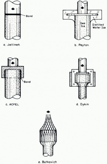
Fig. 22. Methods used for uniaxial tensile tests on ice.

The difficulty of making direct uniaxial tensile tests on ice is evidenced by the popularity of indirect tests, chiefly diametral compression and beam bending tests. However, these indirect tests are no substitute for the uniaxial test for the following reasons:

• (a) It is usually necessary to compute the peak stresses that are assumed to cause failure from linear elastic theory, with equal moduli for tension and compression.

• (b) It is usually necessary to assume that failure is determined by the greatest principal stress, and is unaffected by the values of the other two principal stresses.

• (c) The percentage volume of the total specimen which is subjected to the peak tensile stresses is often very small, and in many cases is only of the order of the grain or flaw size.

• (d) There are often steep stress gradients in the failure zone.

Of the indirect tensile tests in present use, the beam bending test is perhaps the one most widely used. However, it has been recognized for many years that the beam bending test does not measure uniaxial tensile strength; the value calculated as the stress in the lower fibres of the beam is termed the “modulus of rupture”, which for most materials substantially exceeds the uniaxial tensile strength. A detailed study of diametral compression testing (Reference Mellor and HawkesMellor and Hawkes, 1971) has shown that, provided certain experimental conditions are met, the Brazil test (diametral compression of a solid disc) gives an acceptable measure of the uniaxial tensile strength for typical rocks. For ice, however, it gives a strength value far lower than the uniaxial tensile strength. The reasons for this anomaly are not yet clear, although the low ratio of compressive strength to tensile strength for ice may well be involved. The same diametral compression study brought out serious deficiencies in the ring tensile test, and led to a conclusion that any correspondence between ring tensile strength and uniaxial tensile strength is largely coincidental. However, the ring test may give an approximation to the modulus of rupture when the ratio of internal to external diameter for the specimen is sufficiently large.

The uniaxial compressive tests suggest that, for ice, valid tests on simple cylindrical specimens are very difficult to achieve. In the present work considerable care was exercised in specimen preparation and testing, but axial cleavage occurred and measured strength was lower than the strength measured on dumbbell specimens. In previous work, and in work done by others, axial cleavage has been a common mode of failure, and reported values for uniaxial compressive strength of various types of ice (Reference ButkovichButkovich, 1954, Reference Butkovich1959: Reference KaplarKaplar, 1954; Reference Mellor and SmithMellor and Smith, 1966; Reference PeschanskiyPeschanskiy, 1967; Reference Sayles and EpanchinSayles and Epanchin, unpublished;) seem rather low. In testing brittle solids generally, platen surfaces and specimen ends have to meet fine tolerances (platen faces flat to better than 10⁻² mm, specimen ends flat to within about 10⁻² mm) if there is to be any guarantee of valid test results. With ice specimens it is difficult to meet such standards, either by mechanical grinding or by melting, because of the very high homologous temperature of the material. Freezing a water film between the specimen end and the platen may also be troublesome, since there are complications from freezing strains if the initial water film varies in thickness. Thin platen cushions of non-extrudable material (e.g. paper) may be helpful, but thick extrudable cushions, such as the 3 mm thick rubber sheet used by Reference ButkovichButkovich (1954), cannot be recommended.

Dumbbell specimens apparently overcome the end effect problems that can so easily vitiate compression tests, but they are more difficult to prepare than cylinders.

Since uniaxial compressive strength is a strong function of slrain-rate for the range represented by typical speeds of commercial testing machines, at least at high temperatures, selection of suitable strain-rates or loading rates can be a problem. In engineering studies the test loading rate may be decided by the nature of the practical problem involved, but in more general studies it is not easy to decide upon any single strain-rate, since there is inter-relationship between the effects of strain-rate and temperature which might confuse results. The present limited data suggest that uniaxial compression tests intended to induce elastic strain and brittle fracture ought to be run at strain-rates no less than 10⁻² s⁻¹ at peak stress, or 10⁻³ s⁻¹ average rate, when temperatures approach the melting point. In terms of stress rate, this is equivalent to about 30 to 50 bar/s, which is a great deal higher than the minimum rate of 0.5 bar/s recommended by Reference ButkovichButkovich (1958) and followed by others, and the minimum rate of 1.1 bar/s suggested by Gold (1968). The present results (Table I, Figs. 9–11) show that at −7° C there is inelastic straining and ductile failure at stress rates of order 1 bar/s, and measured compressive strength is strongly sensitive to loading rate.

Initial tangent modulus. The mean value of initial tangent modulus measured in compression was 8.76 × 10⁴ bar, which is similar to values obtained by dynamic methods using flexural vibration or elastic wave propagation at sonic frequencies. For bubbly ice at temperatures between −5° and −10° C, dynamic methods give values of Young’s modulus from about 8 × 1G⁴ to 9 × 10⁴ bar (Reference NakayaNakaya, 1959; Reference Bentley, Bentley, Pomeroy and DormanBentley and others, 1957; Reference Grary, Crary, Robinson, Bennett and BoydCrary and others, 1962;. Reference RobinRobin, 1958; Reference GoldGold, 1958; Gold, 1968). Most reported values for “static” Young’s modulus in compression are lower than the dynamic modulus, particularly those resulting from early work, when creep effects were not fully appreciated (see, for example, Reference MantisMantis, 1951). How-ever, it has been found that the static modulus becomes approximately equal to The dynamic modulus (and to the modulus for a single crystal) if temperature is low enough or strain-rate high enough (Reference GoldGold, 1958, 1968).

Initial tangent modulus measured in tension increased with increasing strain-rate, but all values were close to 6 × 10¹ bar. These values are similar to some of the more acceptable reported values for compression (e.g. Reference GoldGold, 1958) and flexural tension (Reference YakuninYakunin, 1968), but well below the dynamic modulus, presumably because strain-rates were not sufficiently high.

Many of the low values of static moduli reported in the literature (≈ 10⁴ bar) undoubtedly represent secant moduli for slow tests, i.e. average slopes for non-linear stress–strain curves. Data from the present tests give abundant evidence of decrease of secant modulus with decreasing strain-rate or increasing test duration (see ratio of peak stress to failure strain, Tables I and II), and the effect has been shown in flexural tests by Reference YakuninYakunin (1968).

Compressive strength. Over the range of strain-rates commonly employed in uniaxial testing, compressive strength is strongly dependent on strain-rate and temperature, so that there is no unique value for strength. Neither is there a unique ratio of compressive strength to tensile strength, since tensile strength is relatively insensitive to changes of strain-rate and temperature.

At the highest strain-rates used in these tests (10⁻² s⁻¹), compressive strength appeared to be tending to a limiting value of approximately 85 to 90 bar at −7° C. It has been suggested, from sketchy experimental evidence (Reference KhomichevskayaKhomichevskaya, 1940; Reference ButkovichButkovich, 1954, Reference Butkovich1958; Reference KorzhavinKorzhavin, 1955; Reference JellinekJellinek, 1957; Reference Mellor and SmithMellor and Smith, 1966; Reference VoytkovskiyVoytkovskiy, 1960; Gold, 1968), that strength actually decreases before settling to a steady value when a critical strain-rate is exceeded, and in the early stages of this work the preliminary results appeared to support this contention. However, it was later found that the apparent drop in compressive strength at high loading rate was actually a consequence of imperfect testing technique—the apparent drop in strength disappeared when specimens were prepared and tested with greater care.

The highest observed value for the ratio of compressive strength to tensile strength was approximately 4 (at 10⁻² s⁻¹ and −7° C). This is smaller than the value of 8 predicted by simple Griffith theory for fracture of brittle materials, and considerably smaller than values found for typical rocks (8 to 20). Reference LavrovLavrov (1965) gave a compression/tension ratio for columnar ice of 9, but the strength values which give the ratio are not too convincing. A low compression/tension ratio for ice has significant bearing on problems involving failure criteria.

Taking into account the fact that bubbly ice tends to be weaker than clearer types of pure ice, most reported values (Mantis, 1957, Reference ButkovichButkovich, 1954, Reference Butkovich1955, Reference Butkovich1959; Reference KaplarKaplar, 1954, Reference VoytkovskiyVoytkovskiy, 1960; Reference LavrovLavrov, 1965; Reference Mellor and SmithMellor and Smith, 1966; Reference PeschanskiyPeschanskiy, 1967; Reference Sayles and EpanchinSayles and Epanchin, unpublished) seem low in comparison with the results obtained here from dumbbell specimens. Some of these reported low values (e.g. Reference Mellor and SmithMellor and Smith, 1966) are undoubtedly erroneous results produced by poor testing technique.

Tensile strength. A significant result of the tensile tests is the demonstrated insensitivity to strain-rate over more than 5 orders of magnitude. This suggests that tensile strength might also be insensitive to temperature, as indeed it appears to be from the limited available data (Reference Wilson and HorethWilson and Horeth, 1948; Reference ButkovichButkovich, 1954; Reference FrankensteinFrankenstein, 1959; Reference HitchHitch, 1959; also unpublished records of tests on ice by L. Hanson of U.S.A. C.R.R.E.L.).

Very few direct measurements of uniaxial tensile strength have been made for ice, and what values are available seem low in comparison with the present results. Reference ButkovichButkovich (1954) obtained a strength of about 14 bar for clearFootnote ^* ice at −5° to −10° C, using the method illustrated in Fig. 22e. Reference KaplarKaplar’s (1954) results, obtained by the method illustrated in Fig. 22c, give a mean value of about 13 bar for clear ice at −6.5° C after rejection of data for specimens that broke in the end cups. A value of 2.75 bar for columnar ice at some unspecified temperature was obtained by Reference LavrovLavrov (1965), who pulled prismatic specimens.

Because direct uniaxial tensile tests are difficult to make, most of the tensile strength data for ice have been obtained from indirect tests, and as already stated, these can be misleading. Following a detailed study of diametral compression testing, the writers used the Brazil test to measure tensile strength indirectly at −7° C (Reference Mellor and HawkesMellor and Hawkes, 1971), obtaining mean apparent tensile strengths in the range 3.3 to 5.9 bar for machine speeds from 8.33 × 10⁻⁴ to 8.33 × 10⁻¹ mm/s. Unpublished data by Hanson give mean Brazil tensile strengths from 2.9 to 4.2 bar for bubbly ice at −10° C, and from 2.2 to 4.0 bar for clear ice at temperatures from −10.5° to −14° C. Data by Reference ButkovichButkovich (1959) give mean Brazil tensile strength as 4.1 bar for bubbly ice at −5° C, although Butkovich himself multiplied his results by a factor of 6. Thus it seems certain that the Brazil test, when applied and interpreted in the accepted manner, gives strength values for ice that are far lower than the uniaxial tensile strength.

The writers also made ring tests on bubbly ice at −7° C, varying the ratio of internal to external diameter from 0 to 0.25 and varying machine speed from 8.33 × 10⁻⁴ to 8.33 × 10⁻¹ mm/s (Reference Mellor and HawkesMellor and Hawkes, 1971). Calculated ring-tensile strength was strongly dependent on both diameter ratio and machine speed, and mean values ranged from 11 to 44 bar. From these results, and from a detailed theoretical and experimental study of the ring test for rocks in general, it was concluded that the ring test does not give a valid measure of the tensile strength of ice. Furthermore, it is doubtful whether it even gives a self-consistent index of tensile strength. Some reported mean values of ring-tensile strength for ice are: 21 to 36 bar (clear ice, −5° to −35° C, Reference WeeksWeeks, 1961), 10 to 32 bar (clear ice, 0° to −20° C, Hanson), 15 to 26 bar (bubbly ice, −0.5° to −20° C, Hanson), 17.5 to 29 bar (bubbly ice, −5° C, Reference ButkovichButkovich, 1959), 14 to 19 bar (clear ice, 0° to −0.5° C, personal communication from G. E. Frankenstein). Most of the data show broad scatter.

Beam bending tests are widely used to provide a measure of tensile strength for brittle materials, even though they suffer from significant and well-known deficiencies. In recognition of the fact that they do not measure bulk uniaxial tensile strength, strength measured by beam tests is termed the “modulus of rupture”. For most brittle materials modulus of rupture is greater than uniaxial tensile strength. Some reported mean values for the modulus of rupture of ice are: 12.5 to 14.5 bar (clear ice, −1.7° to −9.5° C, Reference BrownBrown, 1926), 12.5 to 17.5 bar (clear ice, 0° to −22° C, Reference Wilson and HorethWilson and Horeth, 1948), 12 to 16 bar (clear ice, −5° to 20° C, Reference HitchHitch, 1959), 22.5 bar (bubbly ice, −5° C, Reference ButkovichButkovich, 1959), 13.5 to 14.5 bar (bubbly ice, −3° to −12° C, Reference PeschanskiyPeschanskii, 1967), 21 to 35 bar (clear ice, −12° to −15° C, Reference PeschanskiyPeschanskii, 1967), 13 to 27 bar (clear ice, small beams, −0.2° to −15° C, Reference FrankensteinFrankenstein, 1959), 2 to 7 bar (clear ice, large beams and cantilevers, 0° to −19° C, Reference FrankensteinFrankenstein, 1959).

Transition from ductile yield to brittle fracture. Since there are practical lower limits of strain-rate for constant rate tests, it would be helpful if creep tests could be interpreted so as to give “strength” data for the ductile regime. There appears to be at least implicit recognition of a relation between the results of constant stress creep tests and constant strain-rate strength tests for ductile materials, with the relaxation of stress after yielding in a constant strain-rate test being identified with tertiary creep in the classical creep test (e.g. Reference HigashiHigashi, 1967; Reference Dillon, Andersland and ŌuraDillon and Andersland, 1967). Halbrook (reported by Gold, 1968) observed that the yield strain in constant strain-rate tests on ice was approximately the same as the strain for onset of tertiary creep in constant stress tests. For complete consistency, however, it might be better to associate the peak yield stress of the constant rate test with the mid-point of secondary creep in the constant stress test, regarding the latter as a point of inflection.

In view of the probable relationship between the two tests, it seems legitimate to use data from both types of test to examine the limiting stress–strain-rate relationship for a wide range of strain-rates, and to provide some information on the ductile/brittle transition. In Fig. 19 and 23 tensile and compressive strengths from the present tests have been plotted as functions of strain-rate, and the plot has been extended to lower ranges of strain-rate by plotting stress against minimum (secondary creep) strain-rate for previous creep tests on ice of the same type. Thus the graphs show the maximum value of the stress/strain-rate ratio for each type of test. It is assumed that the compressive creep data represent both compressive and tensile behaviour; Reference SteinemannSteinemann (1958) found no significant difference between creep rates in compression and tension, and there is no theoretical expectation of a significant difference if straining is controlled by the octahedral shear stress.Footnote ^* Data points for compressive creep were taken from Reference Mellor, Smith and ŌuraMellor and Smith (1967) and Reference Mellor and TestaMellor and Testa (1969[a], Reference Mellor and Testa[b]), making small temperature adjustments where necessary.

Fig. 23. Stress–strain-rate envelope, giving maximum value of stress–strain-rate ratio.

From the log–log plot of Fig. 23 it is seen that there is a smooth transition from the creep data to the strength data, which tends to support the case for the proposed relationship between constant stress and constant rate tests. The combined compression data define a smooth curve over more than 9 orders of magnitude; there are no distinct linear sections and abrupt transitions, such as are sometimes seen in discussion of “power-law” creep, nor is there much indication of a drop in strength attributable to onset of brittle fracture. In tension, an upper limit of stress was reached at a strain-rate of order 10⁻⁴ s⁻¹, although the stress/strain diagrams continued to show noticeable curvature up to about 10⁻³ s⁻¹. In compression, it appears that an upper limit of stress is being reached at a strain-rate of 10⁻² s⁻¹, and at this strain-rate the stress/strain diagrams cease to show noticeable curvature. The curves for tension and compression bifurcate at 10⁻⁶ s⁻¹.

Since there is probably a direct relation between creep and yielding, relationships previously established for secondary creep (Reference Mellor, Smith and ŌuraMellor and Smith, 1967; Reference Mellor and TestaMellor and Testa, 1969[b]) are expected to give dependence of yield stress (or strength) on strain-rate and temperature (Fig. 24).

Fig. 24. Relationships between stress, strain-rate and temperature given by uniaxial compressive creep tests at constant stress.

As already mentioned, there is a widespread belief that strength initially increases with strain-rate, eventually reaching a maximum and thereafter decreasing to an asymptotic limit for high strain-rates. The strength maximum and the strain-rate associated with it tend to be regarded as critical values for a transition from ductile to brittle failure. Reference Korzhavin and PtukhinKorzhavin and Ptukhin (1966) have attempted to explain this behavior by analysis of rheological models. In the present work, the apparent strength drop for high strain-rates disappeared when the testing technique was improved, and the writers are therefore dubious about the reality of this effect. Similar questions might be raised about some of the effects attributed to ductile/brittle transition in other branches of materials testing.

Failure strain. The increase in failure strain with decreasing strain-rate can probably be attributed to creep effects. In Fig. 25 the pure elastic strain to failure, obtained by dividing the peak stress by the initial tangent modulus, is plotted against average strain-rate. For tension the elastic strain to failure shows little variation with strain-rate. For compression, elastic strain to failure increases with increasing strain-rate, roughly in proportion to the increase in peak stress with strain-rate.

Fig. 25. Direct elastic strain as a function of average strain-rate.

Energy input. For some engineering purposes it is of interest to consider the work done on the specimen to cause failure. The energy input per unit, volume required to fail a specimen is Kσ _f ϵ _f, where σ _f is peak stress, ϵ _f is failure strain, and K is a shape factor for the stress/strain curve lying between 0.5 and 1.0. In Fig. 26 the product σ _f ϵ _f is plotted against average strain-rate; since K ≈ 0.5 at the highest strain-rates but nearer 0.75 for the low strain-rates, it can be seen that the work done in failing the specimen increases with decreasing strain-rate. The work done in straining ice elastically (proportional to the square of the peak stress divided by the initial tangent modulus) is recoverable, but not usefully so.

Fig. 26. Relation between the product σ_fϵ_f and average strain-rate.

The power expended in failing specimens (energy input divided by time to failure) increases very strongly with increasing strain-rate (Fig. 27), but there are no abrupt discontinuities that could be associated with a sharp transition from ductile to brittle behavior.

Fig. 27. Relation between (σ_fϵ_f/t_f) and average strain-rate.