


INTRODUCTION
Grapevine development can be divided into periodic (phenological) events, which are influenced strongly by weather and climate (Jones & Davis Reference Jones and Davis2000; Parker et al. Reference Parker, de Cortazar-Atauri, van Leeuwen and Chuine2011; Webb et al. Reference Webb, Whetton, Bhend, Darbyshire, Briggs and Barlow2012). Monitoring key phenological stages is crucial for the production of high-quality grapes and wines (Malheiro et al. Reference Malheiro, Campos, Fraga, Eiras-Dias, Silvestre and Santos2013; Sadras & Moran Reference Sadras and Moran2013). Several morphological and physiological differences between varieties result in variances in phenological timings (Winkler et al. Reference Winkler, Cook, Kliewer and Lider1974). This is an additional challenge for planning management activities with potentially high economic impact for growers (Webb et al. Reference Webb, Whetton and Barlow2008; Chevet et al. Reference Chevet, Lecocq and Visser2011), such as treatment applications (spraying) and harvest (Tomasi et al. Reference Tomasi, Jones, Giust, Lovat and Gaiotti2011; Real et al. Reference Real, Borges, Cabral and Jones2015). Therefore, information on the development stages of different varieties, as well as the early detection of the advancement/delay of these stages, becomes increasingly important (Moriondo et al. Reference Moriondo, Jones, Bois, Dibari, Ferrise, Trombi and Bindi2013).
There are three main grapevine phenological stages commonly considered in the literature (Lorenz et al. Reference Lorenz, Eichhorn, Bleiholder, Klose, Meier and Weber1995): budburst (BUD), flowering (FLO) and veraison (VER). Budburst marks the beginning of grapevine seasonal growth and resumed physiological activity, after a long period of winter dormancy; FLO is crucial for the reproductive cycle, being closely followed by the fruit set stage (Fernandez-Gonzalez et al. Reference Fernandez-Gonzalez, Escuredo, Rodriguez-Rajo, Aira and Jato2011) and VER initiates the ripening stage, which is tied strictly to wine grape quality attributes. The progress of these three stages summarize the main differences in varietal development throughout the growing season (Winkler et al. Reference Winkler, Cook, Kliewer and Lider1974; Fraga et al. Reference Fraga, Amraoui, Malheiro, Moutinho-Pereira, Eiras-Dias, Silvestre and Santos2014a ), which in turn influences wine quality attributes (Jones & Davis Reference Jones and Davis2000).
Climate is a major forcing factor on grapevine development and growth. Amongst the more important climatic factors, air temperature plays a leading role in governing grapevine phenology (Dalla Marta et al. Reference Dalla Marta, Grifoni, Mancini, Storchi, Zipoli and Orlandini2010; Bonnefoy et al. Reference Bonnefoy, Quenol, Bonnardot, Barbeau, Madelin, Planchon and Neethling2013; Bonada & Sadras Reference Bonada and Sadras2015), greatly influencing the timing of phenological stages (McIntyre et al. Reference McIntyre, Lider and Ferrari1982; Neumann & Matzarakis Reference Neumann and Matzarakis2014). Additionally, temperature largely bounds the geographical distribution of grapevines (Fraga et al. Reference Fraga, Malheiro, Moutinho-Pereira, Cardoso, Soares, Cancela, Pinto and Santos2014b ), also showing a deep connection to the variability in grapevine yield (Camps & Ramos Reference Camps and Ramos2012; Bock et al. Reference Bock, Sparks, Estrella and Menzel2013), wine production (Santos et al. Reference Santos, Grätsch, Karremann, Jones and Pinto2013; Fraga et al. Reference Fraga, Malheiro, Moutinho-Pereira and Santos2014c ) and quality (White et al. Reference White, Diffenbaugh, Jones, Pal and Giorgi2006; de Orduna Reference de Orduna2010).
Based on these temperature–grapevine relationships, statistical modelling may be used to predict phenology (de Cortazar-Atauri et al. Reference de Cortazar-Atauri, Brisson and Gaudillere2009; Parker et al. Reference Parker, de Cortazar-Atauri, van Leeuwen and Chuine2011, Reference Parker, de Cortázar-Atauri, Chuine, Barbeau, Bois, Boursiquot, Cahurel, Claverie, Dufourcq, Gény, Guimberteau, Hofmann, Jacquet, Lacombe, Monamy, Ojeda, Panigai, Payan, Lovelle, Rouchaud, Schneider, Spring, Storchi, Tomasi, Trambouze, Trought and van Leeuwen2013; Moriondo et al. Reference Moriondo, Ferrise, Trombi, Brilli, Dibari and Bindi2015). Phenology models are indeed key tools for short-term planning of viticultural activities and for studying long-term climate change impacts (Caffarra & Eccel Reference Caffarra and Eccel2011). Previous studies (van Leeuwen et al. Reference van Leeuwen, Garnier, Agut, Baculat, Barbeau, Besnard, Bois, Boursiquot, Chuine, Dessup, Dufourcq, Garcia-Cortazar, Marguerit, Monamy, Koundouras, Payan, Parker, Renouf, Rodriguez-Lovelle, Roby, Tonietto, Trambouze and Murisier2008; Nendel Reference Nendel2010; Parker et al. Reference Parker, de Cortazar-Atauri, van Leeuwen and Chuine2011; Fila et al. Reference Fila, Gardiman, Belvini, Meggio and Pitacco2014; Neumann & Matzarakis Reference Neumann and Matzarakis2014) applied conventional models based on growing degree-day (GDD) measures. Growing degree-days reflect the amount of accumulated heat above the base temperature of 10 °C (Winkler et al. Reference Winkler, Cook, Kliewer and Lider1974) in each growth stage. However, recent research hints at the limitations of these GDD models, such as the need for site-specific calibration and uncertainties in the temperature threshold (de Cortazar-Atauri et al. Reference de Cortazar-Atauri, Brisson and Gaudillere2009; Caffarra & Eccel Reference Caffarra and Eccel2010, Reference Caffarra and Eccel2011; Parker et al. Reference Parker, de Cortazar-Atauri, van Leeuwen and Chuine2011; Zapata et al. Reference Zapata, Salazar, Chaves, Keller and Hoogenboom2015). Most of these models have been applied to regions where climatic conditions are very different from the Mediterranean-like conditions prevailing in Portugal. Furthermore, it has been shown that temperatures over critical intervals may strongly influence grapevine development, which are not adequately captured by the accumulation of daily temperatures (Malheiro et al. Reference Malheiro, Campos, Fraga, Eiras-Dias, Silvestre and Santos2013).
In the climate change context, several studies have been carried out to investigate its impacts on viticulture. Climate change has the potential to modify this crop markedly, providing additional challenges for wine growers (Jones et al. Reference Jones, White, Cooper and Storchmann2005b ; Moriondo & Bindi Reference Moriondo and Bindi2007; Malheiro et al. Reference Malheiro, Santos, Fraga and Pinto2010; Hannah et al. Reference Hannah, Roehrdanz, Ikegami, Shepard, Shaw, Tabor, Zhi, Marquet and Hijmans2013). Regarding phenology, most studies project earlier phenological timings and shorter intervals under future warmer climates (Jones et al. Reference Jones, Duchêne, Tomasi, Yuste, Braslavska, Schultz, Martinez, Boso, Langellier, Perruchot, Guimberteau and Schultz2005a ; Webb et al. Reference Webb, Whetton and Barlow2007, Reference Webb, Whetton and Barlow2011; Tomasi et al. Reference Tomasi, Jones, Giust, Lovat and Gaiotti2011). However, climate change impacts on viticulture are known to be more tied to regional/local climatic conditions than to large-scale changes (Anderson et al. Reference Anderson, Jones, Tait, Hall and Trought2012; Fraga et al. Reference Fraga, Santos, Malheiro, Oliveira, Moutinho-Pereira and Jones2015b ). Therefore, regional assessments of climate change impacts on vine phenology need to be undertaken. No previous research has been focused on the impacts of climate change on grapevine phenology in the Portuguese wine regions. Hence, a deeper understanding of specific varietal differences in phenology is critical to select the most suitable varieties under future climatic conditions (Duchene et al. Reference Duchene, Huard, Dumas, Schneider and Merdinoglu2010).
The objectives of the present study are threefold: (1) to develop a modelling approach that captures the variability of the main grapevine (mostly native) varieties grown in Portugal; (2) to validate the models using different varieties from different Portuguese regions and compare their accuracy with the more conventional GDD models; and (3) to examine the impacts of climate change on regional grapevine phenology.
MATERIALS AND METHODS
Phenology and climatic data
Phenological data were collected from three different wine-making regions (Fig. 1): Douro (Northeastern Portugal), Vinho Verdes (Minho, Northwestern Portugal) and Lisbon (Centralwestern Portugal). These three regions, with centuries-old wine-making traditions, jointly have an important share of the national wine-making economy. The Douro Demarcated Region (including the Denominations of Origin Douro and Porto) is currently the main viticultural region in the country in terms of wine production and vineyard area (150 million litres and 45 000 ha), followed by Lisbon (90 million litres and 25 000 ha) and the Demarcated Region of Vinhos Verdes (80 million litres and 31 000 ha) (IVV 2013). These world-renowned regions are best known for their Port (Douro) and Vinho Verde wines, of which roughly half of the annual production is exported (IVV 2013).
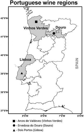
Fig. 1. Location of vineyard sites where data was collected. The delimitations indicate the borders of the winemaking regions in Portugal, as defined by the Portuguese ‘Instituto do Vinho e da Vinha’.
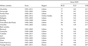
Table 1 describes the 16 grapevine varieties selected for the current study, as well as the corresponding time periods with phenological data. For the Vinhos Verdes region, phenological timings were recorded for the Loureiro (white) variety in the period 2003–2012, from a vineyard located at ‘Arcos de Valdevez’ (41°48′57″N, 8°24′35″W, 70 m a.s.l.). For Douro, phenological data were collected for the Touriga-Franca (red) variety in the period 2001–2011, at ‘Ervedosa do Douro’ (41°10′31″N, 7°32′58″W, 180 m a.s.l.). For Lisbon, data for seven white (Alvarinho, Encruzado, Fernão-Pires, Rabigato, Riesling, Trincadeira-das-Pratas and Viosinho) and seven red (Borraçal, Castelão, Grenache, Jaen, Merlot, Pinot and Tinta-Francisca) varieties were collected from an experimental vineyard located at Dois Portos (DP) (39°02′35″N, 9°10′55″W, 80 m a.s.l.) over the combined period 1991–2011. The timings of BUD, FLO and VER were recorded through field observations following the grapevine descriptors recommended by the Organisation Internationale de la Vigne et du Vin (OIV 2009). The mean calendar day of year (DOY; 1 corresponds to 1 January of a given year) of each phenophase for each variety are also presented in Table 1.
Table 1. Mean day of year (DOY, calendar day of year where 1 corresponds to 1 Jan of a given year) of the BUD (Budburst), FLO (Flowering) and VER (Veraison) for varieties used in the study. Time interval of each series is also shown
The three target regions are characterized by Mediterranean-like climates, with warm dry summers and mild wet winters (Peel et al. Reference Peel, Finlayson and McMahon2007). According to the 1981–2010 climatic norms provided by the Portuguese meteorological office (Instituto Portuguese do Mar e da Atmosfera (IPMA); http://www.ipma.pt), the Vinhos Verdes region typically shows annual mean temperatures of about 15 °C, Douro of 13 °C and Lisbon of 17 °C. For the subsequent analysis, historical records of daily minimum (Tmin), maximum (Tmax) and mean (Tmean) air temperatures, covering the study period and representative of the vineyard sites, were obtained. For Vinhos Verdes, data were obtained from the Sistema Nacional de Informação de Recursos Hídricos (SNIRH) database (http://snirh.apambiente.pt) for the Ponte da Barca weather station, PB (SNIRH code 03G/02C), only 2 km from the vineyard. For the Douro site, due to the lack of local data, climate records were obtained from IPMA for the Vila Real weather station, VR (IPMA code 80567), located about 20 km north-west of the vineyard. For the Lisbon site, data were obtained from the weather station installed in the vineyard, situated at DP.
Phenological models
Each phenophase was modelled for white and red varieties separately, as important differences in the timings of these two types of grape can occur. Although differences in phenological timings may also occur between varieties within these two sub-groups (de Cortazar-Atauri et al. Reference de Cortazar-Atauri, Brisson and Gaudillere2009b ), it was assumed that these differences could be captured by the present models. For this purpose, the varieties with the longest time series of phenological data (Table 1) were selected, i.e. Fernão-Pires (white) and Castelão (red). The full raw time series of the yearly DOY of BUD, FLO and VER were used as dependent variables in linear regression models (least squares estimation).
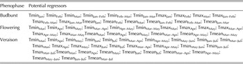
In order to establish statistical relationships between temperature and phenology, monthly averages of daily mean (Tmean), minimum (Tmin) and maximum (Tmax) air temperatures from each site were used as independent variables in the models (predictors). Due to the large number of potential predictors, a stepwise multivariate regression was then undertaken for variable selection (Wilks Reference Wilks2011). The stepwise criterion for forward inclusion and backward removal correspond to P < 0·05 and P < 0·10, respectively. The initial set of potential predictors comprised not only monthly means of Tmin, Tmax and Tmean preceding each phenophase but also multi-month mean temperatures. The full list of potential predictors for each phenophase is shown in Table 2. Based on the predictors selected by the stepwise methodology, a linear model was then fitted for each of the phenological stages. A leave-one-out cross-validation scheme was applied to account for model overfitting. Model residuals were tested using both the Durbin–Watson test and the corresponding autocorrelation function, showing no serial correlation between them (independently distributed).
Table 2. List of potential regressors used for model development
Model performance
For the assessment of model accuracy, the determination coefficient (
 $R_{cv}^2 $
; after a leave-one-out cross-validation) and the root-mean-squared error (RMSE) were estimated. An out-of-sample validation was also performed by applying the developed models to other grapevine varieties grown in the Lisbon region and in the other two regions (Vinhos Verdes and Douro), allowing an inter-regional assessment of the model accuracy. Subsequently, these models were compared against a standard GDD model to test their added-value. The GDD model was computed for both Fernão-Pires and Castelão varieties using the available climatic data from Lisbon. The mean GDD for BUD, FLO and VER stages were computed for 1990–2011, using the standard 10 °C base temperature (Winkler et al.
Reference Winkler, Cook, Kliewer and Lider1974) and an estimated base temperature by applying the minimizing the standard deviation method (Zapata et al. Reference Zapata, Salazar, Chaves, Keller and Hoogenboom2015). For Fernão-Pires the computed base temperature, using this method, was 9·2 °C, while for Castelão it was 8·9 °C. The GDD values, using these base temperatures (10 °C and 9·2/8·9 °C), were then used to determine the yearly DOY of each phenophase. These models were then compared to the newly developed models using
$R_{cv}^2 $
; after a leave-one-out cross-validation) and the root-mean-squared error (RMSE) were estimated. An out-of-sample validation was also performed by applying the developed models to other grapevine varieties grown in the Lisbon region and in the other two regions (Vinhos Verdes and Douro), allowing an inter-regional assessment of the model accuracy. Subsequently, these models were compared against a standard GDD model to test their added-value. The GDD model was computed for both Fernão-Pires and Castelão varieties using the available climatic data from Lisbon. The mean GDD for BUD, FLO and VER stages were computed for 1990–2011, using the standard 10 °C base temperature (Winkler et al.
Reference Winkler, Cook, Kliewer and Lider1974) and an estimated base temperature by applying the minimizing the standard deviation method (Zapata et al. Reference Zapata, Salazar, Chaves, Keller and Hoogenboom2015). For Fernão-Pires the computed base temperature, using this method, was 9·2 °C, while for Castelão it was 8·9 °C. The GDD values, using these base temperatures (10 °C and 9·2/8·9 °C), were then used to determine the yearly DOY of each phenophase. These models were then compared to the newly developed models using
 $R_{cv}^2 $
and RMSE.
$R_{cv}^2 $
and RMSE.
Future projections
Following the phenological model calibration and validation, an analysis of climate change impacts on the phenological timings and intervals was performed. For this purpose, the developed phenological models are then applied to future projections of the mentioned predictors. Four pairs of Global Climate Model/Regional Climate Model simulations (Table 3) were retrieved from the EURO-CORDEX project (Jacob et al. Reference Jacob, Petersen, Eggert, Alias, Christensen, Bouwer, Braun, Colette, Deque, Georgievski, Georgopoulou, Gobiet, Menut, Nikulin, Haensler, Hempelmann, Jones, Keuler, Kovats, Kroner, Kotlarski, Kriegsmann, Martin, van Meijgaard, Moseley, Pfeifer, Preuschmann, Radermacher, Radtke, Rechid, Rounsevell, Samuelsson, Somot, Soussana, Teichmann, Valentini, Vautard, Weber and Yiou2014). All simulations cover the Euro-Atlantic domain at a spatial resolution of 0·11° × 0·11° (~12·5 km). These simulations integrate the Coupled Model Intercomparison Project (CMIP5) and are forced by two Representative Concentration Pathways (RCP) scenarios – RCP4·5 and RCP8·5 for 2006–2100. All models were previously subjected to calibration and bias correction using the Era-Interim reanalysis (Jacob et al. Reference Jacob, Petersen, Eggert, Alias, Christensen, Bouwer, Braun, Colette, Deque, Georgievski, Georgopoulou, Gobiet, Menut, Nikulin, Haensler, Hempelmann, Jones, Keuler, Kovats, Kroner, Kotlarski, Kriegsmann, Martin, van Meijgaard, Moseley, Pfeifer, Preuschmann, Radermacher, Radtke, Rechid, Rounsevell, Samuelsson, Somot, Soussana, Teichmann, Valentini, Vautard, Weber and Yiou2014; Kotlarski et al. Reference Kotlarski, Keuler, Christensen, Colette, Deque, Gobiet, Goergen, Jacob, Luthi, van Meijgaard, Nikulin, Schar, Teichmann, Vautard, Warrach-Sagi and Wulfmeyer2014). As the number of simulations was relatively large, only the ensemble-mean of each scenario for 2020–2090 was used herein to isolate the climate change signal and to assess regional-scale uncertainties.
Table 3. Selected global/regional climate model chains over the period of 2020–2089. All model simulations belong to the Euro-Cordex project (EUR-11 ensemble) and are available at the original grid of 0·11° latitude × 0·11° longitude (spatial resolution of c. 12·5 km)

RESULTS
Present climatic conditions
The three selected wine regions, PB–Vinhos Verdes, VR–Douro and DP–Lisbon, revealed similar temperature seasonality (Fig. 2(a) and (c) and (e)). Ponte da Barca–Vinhos Verdes presented average annual minima of 9·6 °C, maxima of 20·7 °C and mean of 14·7 °C. Vila Real–Douro showed much lower temperatures, with annual minima of 8·8 °C, maxima of 18·9 °C and mean of 13·8 °C. Dois Portos–Lisbon presented temperature values very close to PB–Vinhos Verdes in terms of annual maxima with 20·7 °C, but with a higher minima of 11·1 °C and mean of 15·9 °C. Temperatures are usually highest in August and lowest in January/December in all regions. Vila Real–Douro presented the highest thermal amplitudes (Fig. 2(c)). Dois Portos–Lisbon presented the mildest temperatures during winter (Fig. 2(e)), while PB–Vinhos Verdes exhibited intermediate temperatures. It should be noted that for DP–Lisbon, monthly mean temperatures during the study period (1990–2011) were always above 10 °C, which is commonly considered a temperature threshold for grapevine development (Winkler et al. Reference Winkler, Cook, Kliewer and Lider1974). Regarding the annual mean temperature trends (Fig. 2(b) and (d) and (f)), only Lisbon showed statistically significant trends at P < 0·05 (Fig. 2(f)), with values for Tmean and Tmax of 0·04 and 0·03 °C/year, respectively.
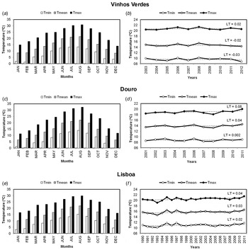
Fig. 2. Left panel: Monthly averages of daily minimum (Tmin), mean (Tmean) and maximum (Tmax) air temperatures registered at (a) Vinhos Verdes, (c) Douro and (e) Lisbon. Right panel: Chronogram of the annual averaged daily minimum (Tmin), mean (Tmean) and maximum (Tmax) air temperatures registered at (b) Vinhos Verdes, (d) Douro and (f) Lisbon.
Phenological models
As mentioned above, the phenological series of one white (Fernão-Pires) and one red (Castelão) variety were selected for a first model calibration. Their phenological time series are shown in Fig. 3. No significant trends were found in the phenological stages of either variety, according to the non-parametric Mann–Kendall test. Regarding the mean DOY of the two grapevine varieties (Table 1), Fernão-Pires tended to reach both BUD and FLO 2–3 days later than Castelão, while Castelão tended to reach VER 2 days later than Fernão-Pires (Table 1). Fernão-Pires showed a lower variability in BUD than Castelão, with interquartile-ranges (IQR) of 10 and 12 days, respectively (Fig. 3). Both varieties showed the same 7-day IQR for FLO. For VER, Castelão and Fernão-Pires show higher inter-annual variability (12 and 10 days of IQR, respectively). The inter-annual variability of these last two events were particularly evident in the year 1997, with an anomalously warm spring. On the other hand, other warmer years, such as 2003, had little influence on the studied phenology, since heat waves occurred mainly after VER (August). Regarding the BUD–FLO interphase length, Fernão-Pires showed a mean duration of 67 days (IQR = 11 days), the same as Castelão (IQR = 10 days). For FLO–VER, Castelão showed higher mean interphase duration than Fernão-Pires (78 and 73 days, respectively) and lower IQR (7 and 8 days, respectively).
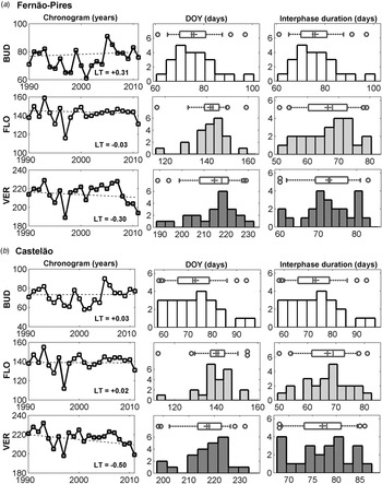
Fig. 3. (a) Left panels: Chronograms of the calendar day of year (DOY) of budburst (BUD), flowering (FLO) and veraison (VER) for Fernão-Pires and over the period of 1990–2011, along with the respective linear trends (LT). No statistically significant LT is found; Middle panels: Histograms of the frequencies of occurrence of DOY for each phenophase. The corresponding mean (+), median (vertical bar), 25th and 75th percentiles (box limits), 9th and 91st percentiles (whiskers) and outliers (circles) are also shown above each histogram; Right panels: the same as on left panel, but for the respective interphase durations. (b) As in (a), but for Castelão.
Following the stepwise process, the most significant predictors were then isolated for modelling the individual phenophases for each variety. For BUD, the identified predictors were TminFeb–Mar for the white model and TminJan–Mar for the red model. For FLO, the same predictor was identified in both models (white and red): TmaxMar–Apr. For VER, the stepwise process identified the largest differences between varieties as well as more than one significant regressor per model. For the white model, the first regressor was TminMar–Jul and the second regressor TmaxMar–Apr. For the red model, the first regressor was TmaxJun–Jul and the second TmeanMar–Apr. The corresponding linear models were significant at a P < 0·001 and are represented in Eqns (1) and (3) for the white varieties and in Eqns (4) and (6) for the red varieties:
 $${\rm BU}{{\rm D}_{{\rm White}}} = {\rm} k{\rm} + {\rm \alpha} \times {\rm Tmi}{{\rm n}_{{\rm Feb} - {\rm Mar}}} $$
 $${\rm FL}{{\rm O}_{{\rm White}}} = {\rm} k{\rm} + {\rm \alpha} \times {\rm Tma}{{\rm x}_{{\rm Mar} - {\rm Apr}}}$$
 $${\rm VE}{{\rm R}_{{\rm White}}} = {\rm} k{\rm} + {\rm \alpha} \times {\rm Tmi}{{\rm n}_{{\rm Mar} - {\rm Jul}}} + {\rm \beta} \times {\rm Tma}{{\rm x}_{{\rm Mar} - {\rm Apr}}}$$
 $${\rm BU}{{\rm D}_{{\rm Red}}} = {\rm} k{\rm} + {\rm \alpha} \times {\rm Tmi}{{\rm n}_{{\rm Jan} - {\rm Mar}}} $$
 $${\rm FL}{{\rm O}_{{\rm Red}}} = {\rm} k{\rm} + {\rm \alpha} \times {\rm Tma}{{\rm x}_{{\rm Mar} - {\rm Apr}}}$$
 $${\rm VE}{{\rm R}_{{\rm Red}}} = {\rm} k{\rm} + {\rm \alpha} \times {\rm Tma}{{\rm x}_{{\rm Jun} - {\rm Jul}}} + {\rm \beta} \times {\rm Tmea}{{\rm n}_{{\rm Mar} - {\rm Apr}}}$$
where k corresponds to the intercept (regression constant), α to the first regressor coefficient and β to the second regressor coefficient, if one exists.
Model validation
Following the identification of the most significant predictors and model development, model accuracy was determined by the previously mentioned metrics (
 $R_{cv}^2 $
and RMSE). Figure 4 depicts observed v. modelled phenological timings (DOY of each phenological event). Overall, the models performed very well, with high
$R_{cv}^2 $
and RMSE). Figure 4 depicts observed v. modelled phenological timings (DOY of each phenological event). Overall, the models performed very well, with high
 $R_{cv}^2 $
and relatively low RMSE for all phenological stages. The FLO and VER models performed better than BUD models in depicting the observed DOY for both varieties, with lower
$R_{cv}^2 $
and relatively low RMSE for all phenological stages. The FLO and VER models performed better than BUD models in depicting the observed DOY for both varieties, with lower
 $R_{cv}^2 $
but similar accuracy (RMSE). The BUD models showed an
$R_{cv}^2 $
but similar accuracy (RMSE). The BUD models showed an
 $R_{cv}^2 $
of 0·63 for Fernão-Pires and of 0·69 for Castelão. Nonetheless, the RMSE for these models was low (4–5 days). The FLO models for both varieties showed higher accuracy, with an
$R_{cv}^2 $
of 0·63 for Fernão-Pires and of 0·69 for Castelão. Nonetheless, the RMSE for these models was low (4–5 days). The FLO models for both varieties showed higher accuracy, with an
 $R_{cv}^2 $
of 0·79 and RMSE lower than 4 days. For VER, the models showed an
$R_{cv}^2 $
of 0·79 and RMSE lower than 4 days. For VER, the models showed an
 $R_{cv}^2 $
of 0·77 for Fernão-Pires (RMSE = 5 days) and of 0·88 for Castelão (RMSE < 3 days). Comparing the results of the newly developed models against a standard GDD model (Table 4), the former tended to out-perform the latter, showing higher
$R_{cv}^2 $
of 0·77 for Fernão-Pires (RMSE = 5 days) and of 0·88 for Castelão (RMSE < 3 days). Comparing the results of the newly developed models against a standard GDD model (Table 4), the former tended to out-perform the latter, showing higher
 $R_{cv}^2 $
and lower RMSE, for both varieties and all phenological stages.
$R_{cv}^2 $
and lower RMSE, for both varieties and all phenological stages.
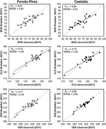
Fig. 4. Left panel: Scatterplots of modelled v. observed calendar day of year (DOY) of budburst (BUD), flowering (FLO) and veraison (VER) for Fernão-Pires over the period 1990–2011 (22 years). The corresponding linear regression line is also plotted. Right panel: the same as on left panel, but for Castelão.
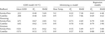
Table 4. Comparison between the growing degree-day model (GDD), minimizing standard-deviation (
sd
) model, along with the calculated base temperature, and regression models, for each phenophase of Fernão-Pires and Castelão. Accuracy parameters for all models are shown:
 $R_{cv}^2 $
and RMSE
$R_{cv}^2 $
and RMSE
For validation purposes, the same models were then applied to other varieties growing not only in the Lisbon wine region (Tables 5 and 6), but also in Vinhos Verdes and Douro (Table 7). In general, for Lisbon, the model performance was very high for all phenological stages and varieties. White varieties showed, on average, higher performance in BUD and VER and red varieties in FLO. Nevertheless, the performance of the BUD model is slightly lower than of the FLO and VER models. Average
 $R_{cv}^2 $
for BUD white/red models was 0·70/0·85 and RMSE of 4/3 days. The FLO models showed the best performances, with a varietal average
$R_{cv}^2 $
for BUD white/red models was 0·70/0·85 and RMSE of 4/3 days. The FLO models showed the best performances, with a varietal average
 $R_{cv}^2 $
of 0·87/0·89 (white/red varieties) and RMSE of 2–5 days. The VER models show average white/red
$R_{cv}^2 $
of 0·87/0·89 (white/red varieties) and RMSE of 2–5 days. The VER models show average white/red
 $R_{cv}^2 $
of 0·86/0·82 and average RMSE of 5/4 days.
$R_{cv}^2 $
of 0·86/0·82 and average RMSE of 5/4 days.
Table 5. White grapevine phenology model for six varieties grown in the Lisbon winemaking region. The
 $R_{cv}^2 $
, root-mean-square error (RMSE, in days), k – intercept, α – first regressor coefficient and β – second regression coefficient are also shown. The independent variables for modelling each phenophase–variety pair are shown in Eqns (1) and (3)
$R_{cv}^2 $
, root-mean-square error (RMSE, in days), k – intercept, α – first regressor coefficient and β – second regression coefficient are also shown. The independent variables for modelling each phenophase–variety pair are shown in Eqns (1) and (3)
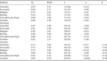
Table 6. Red grapevine phenology model for six varieties grown in the Lisbon winemaking region. The
 $R_{cv}^2 $
, root-mean-square error (RMSE, in days), k – intercept, α – first regressor coefficient and β – second regression coefficient are also shown. The independent variables for modelling each phenophase–variety pair are shown in Eqns (4) and (6)
$R_{cv}^2 $
, root-mean-square error (RMSE, in days), k – intercept, α – first regressor coefficient and β – second regression coefficient are also shown. The independent variables for modelling each phenophase–variety pair are shown in Eqns (4) and (6)
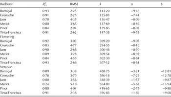
Table 7. Phenology models applied to varieties in other viticultural regions: Loureiro from Vinhos Verdes region (white variety) and Touriga-Franca from Douro region (red variety). The
 $R_{cv}^2 $
, root mean square error (RMSE, in days), k – constant, α – first regressor coefficient and β – second regression coefficient are also shown
$R_{cv}^2 $
, root mean square error (RMSE, in days), k – constant, α – first regressor coefficient and β – second regression coefficient are also shown
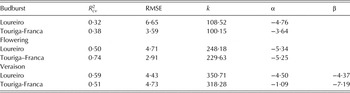
When applying the same models to other varieties growing in other regions (Table 7), model performance generally decreased (
 $R_{cv}^2 $
), but the accuracy (RMSE) remained almost unchanged, with the exception of the BUD model for Loureiro, which exceeded 6 days. Generally, BUD models (as previously) showed the lowest
$R_{cv}^2 $
), but the accuracy (RMSE) remained almost unchanged, with the exception of the BUD model for Loureiro, which exceeded 6 days. Generally, BUD models (as previously) showed the lowest
 $R_{cv}^2 $
of the three phenophase models, with 0·32 for Loureiro (white) and 0·38 for Touriga-Franca. For FLO, the model showed a relatively high performance for Touriga-Franca (
$R_{cv}^2 $
of the three phenophase models, with 0·32 for Loureiro (white) and 0·38 for Touriga-Franca. For FLO, the model showed a relatively high performance for Touriga-Franca (
 $R_{cv}^2 $
= 0·74), but much lower for Loureiro (
$R_{cv}^2 $
= 0·74), but much lower for Loureiro (
 $R_{cv}^2 $
= 0·50). For the VER model, the performance was similar in both regions/varieties, with an
$R_{cv}^2 $
= 0·50). For the VER model, the performance was similar in both regions/varieties, with an
 $R_{cv}^2 $
of 0·59 for Loureiro and of 0·51 for Touriga-Franca. Despite the relatively low performance of the BUD model when applied to other regions/varieties, the FLO and VER models explained more than 50% of the represented variance in the phenological timings, which was a noteworthy outcome.
$R_{cv}^2 $
of 0·59 for Loureiro and of 0·51 for Touriga-Franca. Despite the relatively low performance of the BUD model when applied to other regions/varieties, the FLO and VER models explained more than 50% of the represented variance in the phenological timings, which was a noteworthy outcome.
Temperature projections
Analysis of future projections for air temperature in mainland Portugal revealed a strong warming trend (Fig. 5). Therefore, for the sake of succinctness, only the temperature projections for the main predictors of the phenological models in the Lisbon wine region will be analysed, as similar warming trends are expected for Vinhos Verdes and Douro (cf. Fig. 5). Temperature projections for experiments under the RCP4·5 and RCP8·5 scenarios reveal enhanced upward/warming trends with respect to recent-past trends (Fig. 6): RCP4·5 shows a significant increase of 0·01–0·02 °C/year while the RCP shows increases of 0·03–0·05 °C/year for the selected predictors. Therefore, based on these projections, the most severe emission scenario (RCP8·5) shows the highest warming trends, as expected.
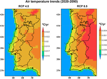
Fig. 5. Ensemble mean air temperature trends (annual mean temperature; °C/year) calculated using the EURO-CORDEX simulations over the period of 2020–2090 and under the RCP 4·5 (left panel) and RCP 8·5 (right panel). Colour online.
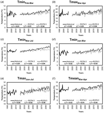
Fig. 6. Chronogram of historical observations (1990–2011) in the Lisbon site and corresponding future projections (2020–2090 under RCP4·5 and RCP 8·5) from the EUR-11 4-member ensemble (cf. Table 3) and for: (a) February–March average daily minimum temperature (TminFeb–Mar); (b) March–April average daily maximum temperature (TmaxMar–Apr), (c) March–July average daily minimum temperature (TminMar–Jul), (d) January–March average daily minimum temperature (TminJan–Mar), (e) June–July average daily maximum temperature (TmaxJun–Jul) and (f) March–April average daily mean temperature (TmeanApr–Mar).
Phenological projections
An analysis of the phenological projections was performed taking into account the period of 2040–2070, in comparison to the current (1991–2011) phenological observations. For all varieties studied, the mean DOY of all phenological timings and intervals showed advances, i.e. earlier timings (Fig. 7). The advancement was more pronounced for scenario RCP8·5 than for RCP4·5 and for the VER stage. Both white and red varieties seemed to be equally affected in the FLO and VER stage, but differently in the BUD stage. For BUD, the advance was slightly more pronounced in the red varieties: 1–5 v. 1–3 days in the white varieties (Fig. 7). The FLO model showed 2–6 days advancement, while VER showed the largest changes, with an advance of 6–14 days depending on future scenario. Concerning specific varietal changes, Fernão-Pires and Grenache showed the largest advances, while Encruzado and Jaen showed the smallest advances of all varieties studied. Future changes hint at significant shortenings of the phenological timings and intervals, while the enhanced warming conditions for grapevine growth will contribute to longer growing seasons. A reduction of 1–2 days could be expected in BUD–FLO for red varieties and 1–3 days for white varieties. This red/white difference can be explained by the more pronounced advancement of the red varieties at the BUD timings. For the FLO–VER interval, a 4–8-day shortening is projected under the RCP4·5–RCP8·5 scenarios.
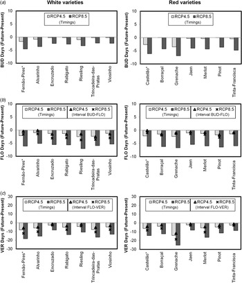
Fig. 7. Left panel: Differences (Future – Present: 2040–2070 minus 1990–2011) in the number of days required to reach (a) budburst (BUD), (b) flowering (FLO) and (c) veraison (VER) for the white varieties (Fernão-Pires, Alvarinho, Encruzado, Rabigato, Trincadeira-das-Pratas and Viosinho). Right panel: The same as on the left panel, but for the red varieties (Castelão, Borraçal, Grenache, Jaen, Merlot, Pinot and Tinta-Francisca).
DISCUSSION
The present study focused on model development for both short-term phenological prediction and long-term climate change impact assessment: it investigates comprehensive changes in future climate under the emission scenarios RCP4·5 and RCP8·5 and their impact on grapevine phenology. Several previous studies have highlighted the impact of climate change on phenology, such as earlier phenophases and shorter intervals (Webb et al. Reference Webb, Whetton and Barlow2007; Hall & Jones Reference Hall and Jones2009; Duchene et al. Reference Duchene, Huard, Dumas, Schneider and Merdinoglu2010). However, no studies focusing on climate change impact on the phenology of Portuguese grapevine varieties has been undertaken so far. Furthermore, no previous phenological model has been simultaneously applied to several varieties of different wine-making regions in Portugal.
Using the longest available phenological records in Portugal, a modelling approach was developed accounting for a broad number of varieties and regions. The model was successful in predicting the phenological timings of BUD, FLO and VER. Overall, for the 16 varieties studied, the average
 $R_{cv}^2 $
for BUD was 0·71, for FLO 0·83 and for VER 0·78. For all phenological stages, the average RMSE was < 5 days in most cases, but for one variety (Loureiro) at BUD. These outcomes are a noteworthy progress, being also comparable, in terms of model accuracy, to other studies in other European wine-making regions (Bindi et al. Reference Bindi, Miglietta, Gozzini, Orlandini and Seghi1997; de Cortazar-Atauri et al. Reference de Cortazar-Atauri, Brisson and Gaudillere2009; Caffarra & Eccel Reference Caffarra and Eccel2010; Parker et al. Reference Parker, de Cortazar-Atauri, van Leeuwen and Chuine2011, Reference Parker, de Cortázar-Atauri, Chuine, Barbeau, Bois, Boursiquot, Cahurel, Claverie, Dufourcq, Gény, Guimberteau, Hofmann, Jacquet, Lacombe, Monamy, Ojeda, Panigai, Payan, Lovelle, Rouchaud, Schneider, Spring, Storchi, Tomasi, Trambouze, Trought and van Leeuwen2013).
$R_{cv}^2 $
for BUD was 0·71, for FLO 0·83 and for VER 0·78. For all phenological stages, the average RMSE was < 5 days in most cases, but for one variety (Loureiro) at BUD. These outcomes are a noteworthy progress, being also comparable, in terms of model accuracy, to other studies in other European wine-making regions (Bindi et al. Reference Bindi, Miglietta, Gozzini, Orlandini and Seghi1997; de Cortazar-Atauri et al. Reference de Cortazar-Atauri, Brisson and Gaudillere2009; Caffarra & Eccel Reference Caffarra and Eccel2010; Parker et al. Reference Parker, de Cortazar-Atauri, van Leeuwen and Chuine2011, Reference Parker, de Cortázar-Atauri, Chuine, Barbeau, Bois, Boursiquot, Cahurel, Claverie, Dufourcq, Gény, Guimberteau, Hofmann, Jacquet, Lacombe, Monamy, Ojeda, Panigai, Payan, Lovelle, Rouchaud, Schneider, Spring, Storchi, Tomasi, Trambouze, Trought and van Leeuwen2013).
The models developed out-performed the classic GDD models. Although the GDD models are currently standard in the wine-making industry (Winkler et al. Reference Winkler, Cook, Kliewer and Lider1974; Fraga et al. Reference Fraga, Costa, Moutinho-Pereira, Correia, Dinis, Gonçalves, Silvestre, Eiras-Dias, Malheiro and Santos2015a ; Zapata et al. Reference Zapata, Salazar, Chaves, Keller and Hoogenboom2015), several limitations to their applicability have been pointed out. Some studies highlight that the GDD calculation is site-specific and cannot be extrapolated to other regions (de Cortazar-Atauri et al. Reference de Cortazar-Atauri, Brisson and Gaudillere2009; Caffarra & Eccel Reference Caffarra and Eccel2010). Other findings demonstrate that the 10 °C base temperature in GDD models may not represent a suitable threshold for all varieties and wine-grape growing regions (Parker et al. Reference Parker, de Cortazar-Atauri, van Leeuwen and Chuine2011; Zapata et al. Reference Zapata, Salazar, Chaves, Keller and Hoogenboom2015). The newly developed models also outperformed the GDD models based on optimized temperature thresholds. These results, obtained for three main wine regions in Portugal, suggest that phenology exhibits a stronger relationship with temperature averages in certain specific periods than with the summations. In fact, key physiological and biochemical processes, such as the remobilization of stored starch and supply of sugar from BUD to FLO, from the permanent structure of the vine to shoot and leaf growth, are initiated by optimum temperatures, promoting expansion and differentiation (Keller Reference Keller2010b ).
The key periods in which phenological development is linearly tied to air temperature are herein identified, confirming the existence of significant links between grapevine phenological timing and temperature in the preceding months, in agreement with previous studies (Malheiro et al. Reference Malheiro, Campos, Fraga, Eiras-Dias, Silvestre and Santos2013). Minimum temperatures from January/February to March have been shown to have a strong influence on BUD timings. Nonetheless, this stage proved to be more difficult to model, which may be due to the influence of viticultural practices, such as pruning date (Martin & Dunn Reference Martin and Dunn2000) or insufficient winter chill (Webb et al. Reference Webb, Whetton and Barlow2007). Maximum temperatures from March to April show a linear relationship with FLO, in agreement with other studies (Bock et al. Reference Bock, Sparks, Estrella and Menzel2011; Tomasi et al. Reference Tomasi, Jones, Giust, Lovat and Gaiotti2011). The VER timings and associated predictors show the highest variability of all phenophases. In addition, the main climatic drivers for this phenophase differ for white and red varieties. For white varieties, the minimum temperatures from March to July and the maximum temperatures from March to April are the strongest climatic drivers. For red varieties, the main driving factors are the maximum temperature from June to July and the mean temperature from March to April. Further, the second regressor (March–April temperatures) coincides with the FLO main climatic driver, highlighting a link between these two phenophases (FLO and VER). In summary, strong links between BUD and winter temperatures, FLO and spring temperatures and VER with spring–summer temperatures were found.
The models showed lower performance when applied to other grapevine varieties growing in other regions in Portugal (Vinhos Verdes and Douro). This result suggests that models need to be locally calibrated in order to optimize their performance. However, lower accuracy in these two regions can be partially attributed to the location of the corresponding weather stations (data used) outside the vineyard, which was reported to have a strong impact on modelling results (Olsson & Jönsson Reference Olsson and Jönsson2015). In Douro, the weather station is 20 km away from the vineyard site, thus being a likely source of errors.
Climate change projections applied to the selected models indicate that future warming will lead to earlier phenological timings and intervals. These outcomes suggest that the VER will have the strongest change, occurring about 2 weeks earlier. The earlier timings of these three phenophases can together reduce the grapevine development cycle considerably. These results are in agreement with recent studies worldwide, such as Duchene & Schneider (Reference Duchene and Schneider2005) for France, Jones (Reference Jones2005) for the USA, Webb et al. (Reference Webb, Whetton and Barlow2007) and Petrie & Sadras (Reference Petrie and Sadras2008) for Australia and Bock et al. (Reference Bock, Sparks, Estrella and Menzel2011) for Germany. These shifts towards earlier phenophase onsets can potentially result in changes to the currently established wine characteristics and typicity. In effect, expected warming may result in unbalanced wines, with high alcohol content and excessively low acidity, altered colour and aroma (Jones et al. Reference Jones, White, Cooper and Storchmann2004a ; Malheiro et al. Reference Malheiro, Campos, Fraga, Eiras-Dias, Silvestre and Santos2013). The potential effects of climate change are not exclusively limited to the reported warming trend. Other consequences projected for the Mediterranean region include higher water stress (Moriondo & Bindi Reference Moriondo and Bindi2007; Fraga et al. Reference Fraga, Santos, Malheiro, Oliveira, Moutinho-Pereira and Jones2015b ) and increased frequency of climate extremes (Santos & Corte-Real Reference Santos and Corte-Real2006; Santos et al. Reference Santos, Corte-Real, Ulbrich and Palutikof2007; Keller Reference Keller2010a ), including in Portugal (Costa et al. Reference Costa, Santos and Pinto2012; Andrade et al. Reference Andrade, Fraga and Santos2014). Extreme weather events, especially winter/spring weather events such as hail and frost, are projected to inflict important yield losses in several crops (IPCC Reference Field, Barros, Stocker, Qin, Dokken, Ebi, Mastrandrea, Mach, Plattner, Allen, Tignor and Midgley2012). Given their unpredictable nature, they may represent an additional challenge for grapevines in future climates. Nonetheless, some positive impacts are also projected, given that the overall length of the growing season is expected to increase, triggered by enhanced warming from spring to autumn.
CONCLUSIONS
In the present study, phenological models are calibrated for Portuguese grapevine varieties, out-performing standard GDD models in predicting grapevine phenology. These models provide robust results, with relatively high accuracy, enabling their direct application by the winemaking sector. Applied to climate change scenarios, projections of the main grapevine phenological stages are achieved. These projections suggest earlier onsets for all phenological stages, as well as a shortening of the phenophase intervals, but with overall longer growing seasons. Hence, although earlier phenological stages may bring detrimental impacts for growers, some benefits may be acquired from the longer favourable periods for grapevine growth, associated with a later onset of autumn cold weather. Therefore, climate change may bring both negative and positive impacts for grapevine development, influencing its entire vegetative cycle. These findings may help delineating suitable adaptation strategies, such as a more critical varietal selection or adoption of innovative viticultural practices, which may potentiate the future sustainability of the national wine industry.
This study was supported by national funds by FCT – Portuguese Foundation for Science and Technology, under the project UID/AGR/04033/2013. This work was also supported by the project ‘ModelVitiDouro’ – PA 53774″, funded by the Agricultural and Rural Development Fund (EAFRD) and the Portuguese Government by Measure 4·1 – Cooperation for Innovation PRODER programme – Rural Development Programme. The authors thank the Estação de Avisos do Douro (Direcção Regional de Agricultura e Pescas do Norte) (Peso da Régua, Portugal) for providing the Douro's phenological data.


