
Abstract
Computational epidemiology seeks to develop computational methods to study the distribution and determinants of health-related states or events (including disease), and the application of this study to the control of diseases and other health problems. Recent advances in computing and data sciences have led to the development of innovative modeling environments to support this important goal. The datasets used to drive the dynamic models as well as the data produced by these models presents unique challenges owing to their size, heterogeneity and diversity. These datasets form the basis of effective and easy to use decision support and analytical environments. As a result, it is important to develop scalable data management systems to store, manage and integrate these datasets. In this paper, we develop EpiK—a knowledge base that facilitates the development of decision support and analytical environments to support epidemic science. An important goal is to develop a framework that links the input as well as output datasets to facilitate effective spatio-temporal and social reasoning that is critical in planning and intervention analysis before and during an epidemic. The data management framework links modeling workflow data and its metadata using a controlled vocabulary. The metadata captures information about storage, the mapping between the linked model and the physical layout, and relationships to support services. EpiK is designed to support agent-based modeling and analytics frameworks—aggregate models can be seen as special cases and are thus supported. We use semantic web technologies to create a representation of the datasets that encapsulates both the location and the schema heterogeneity. The choice of RDF as a representation language is motivated by the diversity and growth of the datasets that need to be integrated. A query bank is developed—the queries capture a broad range of questions that can be posed and answered during a typical case study pertaining to disease outbreaks. The queries are constructed using SPARQL Protocol and RDF Query Language (SPARQL) over the EpiK. EpiK can hide schema and location heterogeneity while efficiently supporting queries that span the computational epidemiology modeling pipeline: from model construction to simulation output. We show that the performance of benchmark queries varies significantly with respect to the choice of hardware underlying the database and resource description framework (RDF) engine.
1 Introduction
Epidemiology is the study of the distribution and determinants of health-related states or events (including disease), and the application of this study to the control of diseases and other health problems [1,2,3,4,5,6]. Computational and digital epidemiology aims to develop computational models, analytics, and decision support tool to support epidemic science [2, 7]. The science and practice of the discipline has matured steadily over the past decades. Advances in computing and data science have facilitated the development of novel technologies and apps that support epidemic planning and response. These tools are now viewed as important assets for epidemiologists and public health officials. Epidemiologists use such tools to study a number of epidemic policy questions, including forecasting, planning, situational awareness, and intervention analysis; see [4, 8,9,10,11,12,13,14,15,16,17] and the references therein.
1.1 Agent-Based Epidemiological Modeling and Analytics
Aggregate or collective computational epidemiology models that have been studied in the literature for over a century often assume that a population is partitioned into a few subpopulations (e.g., by age) with a regular interaction structure within and between subpopulations. Although useful for obtaining analytical expressions for a number of interesting parameters such as the numbers of sick, infected, and recovered individuals in a population, it does not capture the complexity of human interactions that serves as a mechanism for disease transmission. See [4,5,6, 18, 19] for more details.
Agent-based models (aka network-based models) extend the aggregate models by representing the underlying interactions by dynamic networks. These class of models capture the interplay between the four components of computational epidemiology: (i) individual behaviors of agents, (ii) unstructured, heterogeneous multi-scale networks, (iii) the dynamical processes on these networks, and (iv) contextualized social and pharmaceutical implementable interventions. They are based on the hypothesis that a better understanding of the characteristics of the underlying network and individual behavioral adaptation can give better insights into contagion dynamics and response strategies. Although computationally expensive and data intensive, agent-based epidemiology alters the types of questions that can be posed, providing qualitatively different insights into disease dynamics and public health policies. It also allows policy makers to formulate and investigate potentially novel and context-specific interventions. We refer the reader to [1, 2, 7, 11, 12, 18,19,20] for further discussion on this subject.
Agent-based models and analytics have become increasingly popular and are often the model of choice to study certain kinds of epidemiological questions. They are harder to build, largely due to the expertise in computing and data science needed to build them. For instance, implementing these models on computing clusters and analyzing the outputs produced by such models requires a fair bit of expertise in computing and data science. This has led to the development of web-apps and modeling environments that make it easier for analysts to use such models and analytical tools. Our group was the first group that developed such a web-based modeling and analytics environment. It is called SIBEL—Synthetic Information Based Epidemiological Laboratory Footnote 1; screenshots of the system are shown in shown in Figs. 1, and 2a, b [21]. SIBEL was specifically designed so that epidemiologists can carry out sophisticated what-if studies using agent-based epidemiological models and analytics without becoming computing experts. A few other groups have also begun developing similar modeling and analytics environments; see [22, 23]. Other significant recent related efforts include the following: (i) CDC FluView [24]; (ii) HealthMap [25]; (iii) Texas Pandemic Flu Toolkit [26]; (iv) LANL BARD [27], (v) EpiC [28].

This figure shows the SIBEL web application experiments page. The user sees this page after logging in. This page provides a quick summary of the experiments. If a user clicks the “All” button, then this page shows all the experiments run on SIBEL by various users. Otherwise, it shows only the experiment(s) conducted by the logged in user

Experiment setup facility in SIBEL
1.2 The Need for a Knowledge Base
The input and output datasets arising in the context of developing agent-based modeling environments for epidemics are large, diverse and heterogeneous. They are stored in various formats and over multiple storage devices. This makes the task of developing effective analytical and decision support tools challenging. This motivates the need to develop a knowledge-base (EpiK) to store, link and efficiently retrieve the diverse datasets. For the purposes of this paper, we use the term knowledge base to denote a data management system to represent, organize, collect, store, and integrate structured and unstructured information in a machine-readable form.
The motivation to develop EpiK arose as we were working on SIBEL. To understand this, we briefly describe how systems like SIBEL are used to support a typical case study.
1.2.1 What Is a Case Study?
An in silico epidemiological case study evaluates outcomes generated by a computational experiment. In these experiments, users can specify the following:
-
1.
A social contact network
-
2.
A within-host disease progression model
-
3.
A set of initial conditions
-
4.
A set of interventions
Each intervention requires additional details such as compliance level, sub-populations to which interventions are applied, and under what conditions the interventions take place. The experiment contains one or more sweeping parameter(s) across a user-specified range of values. For example, experiments in a typical study would be divided into one or more cell(s). A cell may have multiple interventions. Vaccination, social distancing, and closing schools are a few examples. In order to arrive at a stochastically robust conclusion, each experiment is run multiple times but with different initial conditions (for example, the number of infectious persons at the beginning of the simulation) [21]. A web portal such as SIBEL provides an easy-to-use and intuitive interface to carry out such an experiment.
1.2.2 An Illustrative Example
A typical case study involves planning for an infectious disease outbreak such as influenza-like illness (ILI). Consider the following hypothetical situation: Alice and Bob are two epidemiologists tasked with carrying out computer experiments to study various what-if scenarios concerning the spread of ILI in the USA. They are particularly interested in understanding the role of interventions in controlling the outbreak. Both Alice and Bob decide to use SIBEL for their computer experiments. As a first step, Alice selects Boston, MA, as a region of interest since reports suggest that it might be one of the first regions to experience an ILI outbreak this season. Bob chooses Houston, TX, as a region of interest, keeping in mind that the last influenza pandemic started in Mexico. Using SIBEL, both select different disease parameter values, including susceptibility, infectivity, and days to recovery. They then choose a complex set of interventions, including school closure, social distancing, and antiviral distributions, and decide how these interventions are implemented (who, when, and for how long). The entire workflow effectively sets up a formal statistical experimental design. Launching the experiments is easy with SIBEL; it involves simply pushing the run button. Alice and Bob do not have to know where the data is stored and where the computation will be carried out. Once the experiments are completed, they can carry out a detailed analysis. Basic results of the experiments are displayed to the user through a set of plots and aggregate statistics.
1.2.3 A More Detailed Epidemic Investigation and Initial Challenges for SIBEL
Suppose, upon completion of the study, Alice seeks to infer additional information about a few infected individuals including their home locations and their daily activities before the time of infection. Alice might also look for infected individuals are known as super-spreaders, while Bob might be interested in the role of critical workers and school-aged children in disease transmission. Both might also want to do a comparative analysis to see the differences and similarities between the epidemics in the two regions. This would help them understand the impact of social networks and the built infrastructure on epidemic dynamics and in turn may help them design and study contextualized intervention policies. Investigations such as the ones above can be cast as workflows involving queries that Alice and Bob write.
To retrieve the results for the abovementioned queries, a user with access to the servers must determine the cell information of the experiment from the SIBEL user interface. Then the system administrator must read the cell directory from the HPC resource. The cell directory contains the configuration file. The configuration file provides the output file location in the HPC resource. The output file provides infector and infectee information and their identification (ID) numbers. The configuration file contains the social network folder path information as well. From there, synthetic population location can be determined and stored in a relational database. By querying that database with the IDs of infected individuals, Alice/Bob can discover activities performed by the infected person in the last few days, the disease transmission between various demographic groups, and their location information. In its current form, SIBEL does not support this kind of enhanced analysis. In other words, answering queries such as this tends to be a manual, tedious, and laborious process because of its use of heterogeneous and fragmented data sources.
1.2.4 Further Challenges as SIBEL Is Used and Grows
A key aspect of SIBEL is its simplicity—public health analysts are trained to make effective use of the system in approximately three hours [21]. Studies that took months and days can now be done in hours using SIBEL. The early days of SIBEL saw significant effort devoted toward making the system user-friendly and toward modeling realistic epidemic situations by scaling the backend simulation engine [29,30,31]. As a result of this effort, SIBEL is used by epidemiologists, computational researchers, and public health experts to model the spread of infectious diseases over large geographical regions with populations of up to 50 million people. We have since performed over 30 case studies requested by our sponsors in many metropolitan areas in the United States. As a recent example, SIBEL was used to support DTRA’s Ebola response efforts in West Africa. SIBEL is constantly evolving; new modeling engines are being added as a part of the backend; new kinds of analysis is supported and new populations and regions are being added.
The continued growth and use of SIBEL have made the problems identified above even more challenging. The output datasets are growing rapidly as analysts use SIBEL routinely. As a result, comparative analysis of experiments and contextual analysis of outcomes that need to reason over both input and output data has become progressively challenging. Data-centric tasks like performing validation, verification, analysis, and model refinement also became cumbersome and challenging. This problem is further exacerbated because the exponential growth in the volume of data is intertwined with heterogeneity (in data types) and fragmentation (in storage) present in the datasets. Heterogeneity in data types is pervasive across the entire spectrum of the discipline, i.e., starting from data acquisition (of surveillance, census, etc.) to analysis of simulation outputs. A typical simulation makes use of a sequence of digital content types including input parameter configurations, raw datasets, result summaries, analyses and plots, documentation, publications, and annotations. A myriad of datasets is generated as a simulation output. SIBEL is distributed and part of a larger ecosystem. Fragmentation of the storage is a major hurdle, primarily arising due to the logistics of maintaining such large datasets and the architecture of the SIBEL infrastructure itself. All these factors contribute toward the current state where organization, querying, annotation, and other services become cumbersome and often infeasible. Small changes to the schema at the storage layer cascade into significant changes in the data access and application layer. EpiK addresses these challenges.
Although the discussion was framed in the context of SIBEL, the issues discussed are generic — all epidemic modeling environments for decision support and planning face similar challenges.
1.3 Contributions
The paper describes EpiK—a knowledge base that can support agent-based epidemiological modeling, analytics, and decision-making. EpiK designed to store, link, and query diverse datasets are arising in epidemic modeling and counterfactual analysis. We focus on agent-based networked models; supporting compartmental models is considerably easier and can be seen as a subcase. EpiK uses modern semantic web technology to unify and link diverse dynamic datasets and represent them in a machine-understandable format. It provides methods for building semantic graphs and provides a query bank to improve analysts’ productivity.
The paper focuses on agent-based epidemiological modeling and analytics of infectious diseases. Extensions to chronic and environmental disease epidemiology will be undertaken subsequently. The use of EpiK to support aggregate modeling is relatively easy.
In Fig. 3, we present the main flow of the agent-based epidemic modeling and analytics. EpiK provides linked access to SIBEL data sources such as synthetic population and contact data, computational experiment setup data, and computational experiment output data. The datasets may contain data of different types, such as demographic, aggregate, and sequence, or may differ in the storage technology (such as ASCII files, binary files), and may be distributed physically across different machines in the network. We discuss two approaches for machine-understandable RDF representations. We show the prospect of virtual and materialized views when developing EpiK.

This figure displays computational networked epidemiology pipeline (CNEP). It has three parts. The first part of the pipeline is “Synthetic Population.” This part handles a synthetic representation of people, household structure, location and various people activities. We employ census, landscan, and other data sources to create statistically identical synthetic population. This part also creates people visitation synthetic graphs (people-people and people-location). The second part of the figure is “Agent-Based Modeling”, which represents the SIBEL tool. Here we employ “People Visitation Synthetic Graphs” generated in the earlier phase. The “Agent-Based Modeling” also uses “Disease Model,” “Initial Condition,” “Intervention,” and “Trigger” information. This part conducts various computational networked epidemiology experiments, and it generates numerous output files. The main file is the “Dendogram” that contains who infected whom’s information. Finally, by using SIBEL analysis facility, the user can perform data analytics on experiment outputs. The EpiCurve and daily mean infections are some examples of the analysis output
A programmatic data access capability is provided to access the data organized within EpiK. This permits data sharing and interoperability and makes it easier for others to build applications on top of the simulation data. The user can execute complex queries over heterogeneous SIBEL contents. We demonstrate the utility of EpiK by developing a query bank. The queries are representative of typical analysis carried out by an epidemiologist during the course of planning or response phase of an epidemic. These queries are based on the 5W1H concept and demonstrate the utility of semantic web technologies. Specific contributions are summarized below.
1. Linked Data Access and Query Execution Framework
A central contribution of EpiK is a federation of all datasets relevant to agent-based epidemiological modeling and analytics using SIBEL—including input, output, and experimental conditions. The proposed framework offers various advantages: (i) linking large amounts of data sources, (ii) linking a variety of data sources, (iii) access to programmatic data, and (iv) query efficiency. The methodology is general—as new datasets arrive, they can be easily integrated with the proposed EpiK framework. Data linking, in EpiK, is achieved through native relational database (RDB) to RDF data mappings. The RDF tools and data mappings are central to our research. This linked data framework, to a large extent, addresses the challenges faced due to heterogeneity in schema, formats, and storage across the datasets in the domain science. The key concept to achieve this end is to define a representation of the datasets that encapsulate both the location and the schema heterogeneity. The proposed framework provides a linked view to access and query end-to-end epidemiology workflow datasets.
2. Native to RDF Mappings (Techniques and Their Trade-Offs)
We study two classes of RDF mappings in this context: value-based and tuple-based. Fundamentally, the difference in these two mappings lies in how relationships among entities are expressed and materialized. Value-based mapping preserves child-parent entities relationships while tuple-based mapping completely ignores it. This paper investigates the trade-offs of the mappings with respect to schema clarity (including ease in understanding the data organization and ability to frame queries), storage cost, and efficiency of answering queries.
3. Query Bank and Benchmarking
We develop a benchmark to evaluate different implementations for a homogeneous query execution framework. The homogeneous query execution framework builds a federation of the disparate datasets and exposes them (using the mappings) as a unified whole. The benchmark is a collection of SPARQL queries over the federated SIBEL data. Collectively, they capture access patterns and workloads that appear frequently in the domain. The queries are representative of real-time epidemiology queries. We use the benchmark to evaluate two kinds of query execution frameworks: one relational engine-based and the second RDF engine-based. Relational engines are space efficient and therefore can scale to very large datasets while RDF engines are query efficient and therefore useful when a real-time response is mandatory.
4. Evaluation of the Design Space for Homogeneous Data Access and Querying Framework
The choice with respect to style of representation (value- vs. tuple-based) combined with the implementation of the execution platform (relational engine-based vs. RDF engine-based) provides us with four possible design points for the proposed platform. Each design point has different trade-offs. This work evaluates all the four possible implementations with respect to the benchmark.
In summary, we provide a solution for how to build a linked database for heterogeneous and federated computational epidemiology data sources. Preliminary evaluation of the framework demonstrates that leveraging semantic web technology (in particular RDF concepts) is an effective strategy for handling data-centric challenges faced in such distributed, multi-user, large-scale computational science. Our approach demonstrates that fast unified access across fragmented datasets is feasible. Different strategies offer trade-offs with respect to storage space or query time. Query execution in a pure RDF engine is faster, but has a large storage cost. On the other hand, in the hybrid relational-RDF engine, we have zero RDF graph storage cost but efficiency is compromised.
2 Related Work
Our work builds on earlier work in scientific data management, digital libraries, and semantic web tools. Scientific data management is a long-standing research field, driven by the fact that most scientific software produces a myriad of specialized data. Early work on scientific data management introduced the concept of a process-oriented scientific database model (POSDBM) [32], which includes two data objects and relation types. This work is extended with key semantic elements of scientific experimentation by Pratt et al. [33].
Shi et al. [34] presents a web-based epidemiology reporting system that uses Google Maps data. Allon et al. [35] describes a leukemia epidemiology study where the data model arises from the experiment based on a relational modeling approach. In the domain of the Semantic Web, tools that map data from the relational model to RDF (and vice versa) have been an active area of research [36,37,38,39,40]. Bertails et al. demonstrates the power of the mapping to treat all of the important features of SQL tables, like cardinality and NULLs, and to yield an RDF graph which preserves the relational information [37]. Hert et al. illustrate ontology-based access to relational databases as discussed in [41]. It describes a mapping language, the translation algorithms, and a prototype implementation. Robert et al. develop a schema ontology for healthcare using reference information model (RIM). This modeling helps better manage healthcare effectiveness data and information set (HEDIS) measures by providing a rule ontology that is matched to the language of the specification [42]. Horrocks et al. propose an ontology-based data access (OBDA) solution for diverse varieties of data management. They describe their efforts in the context of managing disparate Siemens Energy Services datasets; see [43] for further discussion.
Multiple studies have addressed processing queries using mapping [44,45,46]. Bornea et al. [44] describe novel query translation techniques as well. Experiments show that the approach provides good results when compared with current state-of-the-art stores. Groppe et al. describe an SPARQL query optimization technique that uses seven indices to retrieve RDF data quickly [45]. This approach computes joins by dynamically restricting triple patterns, and provides good efficiency. Arenasa et al. introduce a theoretical foundation for faceted search explicitly designed for RDF-based knowledge graphs improved with OWL 2 ontologies. Authors also investigate convenient faceted interfaces [47].
Unification of heterogenous data using semantic tools has been actively studied for biological data [48, 49]. BioPortal provides biomedical ontologies [50]. Federation (or mediation) of physically distributed data sources using RDF (and other semantic constructs) in DartGrid is presented in [51], which provides RDF/OWL to define the mediated ontologies for integration, as well as automatic conversion rules from the relational schema to RDF/OWL descriptions. Kamdar et al. proposes an approach for Ebola virus knowledge-based creation using semantic web technologies [52].
Examples of scientific digital libraries include earthquake simulation repositories [53], embedded sensor network DLs [54], and D4Science II [55]. Barrett et al. describe a data management tool to study infectious diseases [56]. Schriml et al. provide the GeMIna system, that uses epidemiology metadata to identify infectious pathogens and their representative genomic sequences [57]. The VecNet digital library maintains curated data, tagged citations, and articles related to epidemiology [58]. Leidig describes a scientific digital library to manage epidemiology experiments and simulations, but does not provide any specific framework for heterogeneous epidemiology big data management [59].
3 The EpiK: Data Federation and Homogeneous Query Execution Framework
The proposed EpiK consists of three layers: (i) the data layer: datasets (Section 3.1), (ii) the mapping layer (Section 3.2), and (iii) RDF engine and services layer (Section 3.3). See Fig. 4. We discuss each of the layers below.

The proposed EpiK for agent-based epidemic modeling and analytics. It consists of three components/layers. The bottom layer (data layer) presents various computational epidemiology datasets in numerous formats. The middle layer (mapping layer) converts all the relevant data into materialized and virtual RDF graphs through mapping file and D2RQ engine. The top layer (RDF engine and services layer) exposes the materialized RDF graph through Jena TDB [60] and Virtuoso servers [61], and the virtual RDF graph through D2RQ server [62]
3.1 The Data Layer
We start by describing EpiK’s dataset layer; see Fig. 4. Here, we focus on by SIBEL. The datasets are summarized in Fig. 5 and comprise the (i) synthetic population, synthetic people-location network, and synthetic social contact network, (ii) experimental setup data consisting of disease model parameters and intervention specification, and (iii) experimental output data comprising of epidemic curves, dendograms, and various analysis. Table 1 shows the type, size, and format for datasets present in SIBEL [63].

Figure summarizing the type of datasets used as a part of agent-based epidemic modeling and analytics framework pipeline shown in Fig. 3. Here, oval shape represents dataset, and the ontological relationships between various datasets are available just next to the oval. Here synthetic population and network part cover person, household, location, activity, and contact network datasets. The agent-based modeling uses contact network, disease model, intervention, and produces output datasets. The analytical tool covers experiment output analysis related datasets
3.1.1 Synthetic Input Data
Synthetic population and activity data describe individuals and their activities. Synthetic activity data describe activities performed by the individuals, which include travel and visits to locations of work, home, and daily errands. As part of the activity, people come in close contact with other individuals. The contact data capture this information and are central to the study of epidemics. The synthetic population database contains households, persons, activities, and location information. Data are stored in a relational format. Schema descriptions of the synthetic population tables for household, person, and activity, activity location, and home locations are given in Tables 2, 20, 21, 22, and 23. Descriptions of U.S. Census 2000 Public Use Microdata Sample (PUMS) demographic variables are available online at [64].
3.1.2 Disease Manifestation and Intervention Data
Experiments are divided into multiple cells. Each cell characterizes one set of quantified simulation conditions and may have many replicates (10 is typical). Numerous intervention actions are applied to the epidemic simulation for decision making processes. Social distance, school closure, work closure, vaccinations, and antivirals are some of the intervention types. Interventions may be implemented at a predetermined time (e.g., on day 1), or when a certain condition is met (e.g., when 1% of school-aged children are diagnosed). The goal of the intervention is to interrupt disease transmission from one person to another. Interventions may be targeted to specific demographic groups, or subpopulations, such as school-aged children or workers in critical jobs (e.g., first responders). SIBEL experiment setup data are stored in both the relational database and the file system. The relational database mainly stores experiment, analysis, disease model, and intervention information (Tables 24, 25, 26, and 3) [29]. Configuration information is stored in the file system (Table 4).
3.1.3 Output Data
Output data describe the spread of disease through a population. This generally contains three parts [65]. First, it contains a list of infected people along with information about the time and duration of incubation and infection and results of interactions with health care providers such as whether or not they were diagnosed. Second, it contains a set of trees with the initially infected persons as the roots showing the path of infection through the population. This is referred to as a dendogram. Third, it contains a list of interventions and the time at which they were implemented. Multiple dendograms across replicates and cells are used to produce tabular data (e.g., epidemic curves, intervention rankings, and interaction effects, etc.).
The datasets are distributed across several different databases, schemas, file systems, and machines. The scale of the data and use of fragmented storage makes tracking experiment setups and scientific workflows cumbersome and error prone and therefore limits verification and reproducibility of results (Table 4).
3.2 The Mapping Layer
Next, we discuss the second layer in EpiK as depicted in Fig. 4. This layer maps all this.
3.2.1 Why RDF?
Our choice to represent all data using RDF stems from similar considerations by other researchers using RDF in the field of biomedical and health sciences. We briefly discuss the rationale below.
First, epidemiologically relevant datasets come in various forms, are large, and are growing rapidly as SIBEL continues to be used by policy analysts. Often, new kinds of datasets need to be accommodated. This requires frequent schema changes when using relational database management system (RDMS), but easily handles with RDF. Commercial relational databases can be useful in some cases but their cost and licensing rules limits their use and increases the cost of using SIBEL for our customers.
Second, RDF data model is a good choice for the epidemiologists that satisfies the prerequisites listed earlier. It is a standard data model recognized by the World Wide Web Consortium (W3C) [66]. The RDF permits the consolidation of various data models (for example, tree, relational, graph, and so on) and vocabularies [67]. The RDF data model gives dynamic metadata structure in contrast to relational databases. Therefore, RDF is much more suitable for handling the growing graph-oriented dynamic data [67].
Third, RDF-based storage allows us to identify data on the internet with URIs. This allows the creation of globally unique names and is useful as multiple stakeholders across the world use SIBEL with little direct coordination. Using RDF makes it possible to distribute our data as linked open data (LOD) on the internet using RDF data model. This makes it easy to link our datasets to pertinent internal and external datasets from the LOD cloud (for example, BioModels, BioPortal, BioGateway, and BioSamples) [68, 69]. Linking these and other social media datasets is needed in the near future to understand complex questions arising in anti-microbial resistance and phylodynamic analysis.
Fourth, SPARQL is a natural language for studying questions arising in epidemic modeling given that a number of questions pertain to traversing social contact networks or disease dendograms. Complex queries that need multiple combinations in SQL are relatively easy to create in SPARQL [70]. Moreover, transitive closure style queries (e.g., looking for paths in a network) are easier in SPARQL than SQL.
Finally, using RDF allows utilization of a publicly accessible linked data browser, link discovery, semantic web indexes, and diverse representation tools. Very little effort is needed to implement these tools. Rather than creating a personalized graphical user interface (GUI) for data browsing, epidemic experts can utilize current faceted programs to analyze data with the help of basic ontologies [71,72,73,74]. Any change in the data or ontology will automatically reflect in the GUI. Most of these tools are freely available on the web. Although these tools have some limitations, they provide a quick view on top of the data with no cost.
3.2.2 Mapping to RDF
We would like to unify heterogeneous and fragmented CNEP datasets into RDF format. That requires relational to RDF mapping. Several mapping strategies exist in the literature along with tools that use the mapping to build the RDF dataset [36,37,38,39,40]. In this work, we investigate tuple-based and value-based mapping techniques [75]. We use the D2RQ tool to generate the mappings. We consider two types of mapping.
3.2.3 Tuple-Based and Value-based Mappings
In tuple-based mapping, RDB table name is considered as an RDF class name and column name as property name. For each instance of the table a unique blank node is created. Naming of the blank node can be done in various ways but incremental number assignment is the simplest way. Tuple of an instance contains a blank node, a label edge, and a literal. Property name is used as an edge label and each of the property values are used as a literal of the tuple (Fig. 6). Tuple-based mapping uses relational database tables as input and produces RDF graph as output, ignoring the primary key foreign key relationship.

This figure depicts a tuple-based mapping example. Here, we have two datasets (person and household). The tuple-based mapping disregards the primary key and foreign key relationship in RDF mapping
Primary key and foreign key join exists in the database and is preserved in value-based mapping. The input of value-based mapping is relational tables and output is RDF graph with join information. Primary key attribute values are presented by URIs. In value-based mapping the primary key attribute value of the parent object points to the child object (Fig. 7).

This figure illustrates a value-based mapping example. The value-based mapping considers the primary key and foreign key relationship in RDF mapping (dotted arrow in the figure). Here, “HID” is the primary key in the household table and foreign key in the person table
In this paper, we have used tuple-based and value-based mappings. Our choice was based on the following observations. First, both are commonly used mapping schemes in the literature; see [75]. Numerous relational to RDF data conversion approaches are developed on top of tuple-based mapping or a modified version of it. Examples include the following: Relational.OWL [76], DataMaster [77], ROSEX [78], Automapper [79], FDR2 [80], CROSS [81], D2RQ [82], Tether [83], and OntoAccess [41]. Value-based mapping is the simplest form of the relational to RDF mapping approach that preserves primary key and foreign key relationships [75]. The availability of mature tools and our goal of preserving primary and foreign key relationships were important considerations when we made the choice. To the best of our knowledge, this is the first use of RDF graphs for supporting computational networked epidemiological investigations.
Lausen discusses other kinds of mappings, most notably URI-based mappings and object-based mappings to convert RDB into RDF [75]. However, they have certain limitations. In URI-based mapping, primary key values are encoded in the tuple URI. Suppose primary key of a table is a foreign key to another table then one might encounter consistency problems. In object-based mapping, it is hard to find foreign key because it requires property path traversal [84].
Tuple-based and value-based mappings are formally defined below.
Preliminaries
Let S be a relational schema and A(S) = {A 1,...,A k } is the attributes of S. I denotes an instance of S and T = (a 1,...,a k ) represents every tuple of I. We use C S as a class over S with properties \(P(C_{S})=\lbrace P_{S,A_{1}},...,P_{S,A_{k}} \rbrace \). We use F C to denote the finite set of classes. Mapping creates an RDF graph G such that for every tuple T in I create a node n T and an edge (n T ,r d f : t y p e,C S ). Tuple-based and value-based mappings have differences in edge creation.
Tuple-Based Mapping
Let T.A be the value of an attribute A. For every non-null value T.A of T, A ∈ A(S), tuple-based mapping creates an edge \((n_{T}, P_{S,A}, (T.A)_{n_{T},P_{S,A}})\). This type of mapping ignores primary key and foreign key relationships.
Value-Based Mapping
We use C S to denote a child class and C S ′′ for parent class. Let \(C_{S}, C^{\prime }_{S^{\prime }} \in F_{C}\). We write T.A to represent a non-null value of an attribute A over C S and T ′.A ′ for a non-null value of an attribute A ′ over \(C^{\prime }_{S^{\prime }}\). P S,A represents the C S properties and \(P^{\prime }_{S^{\prime },A^{\prime }}\) represents \(C^{\prime }_{S^{\prime }}\) properties. Value-based mapping contains primary key and foreign key relationships information. For that, if T.A of T contains foreign key value and T ′.A ′ of T ′ contains primary key value then an edge (n T ,P S,A ,\((T^{\prime }.A^{\prime })_{n^{\prime }_{T^{\prime }},P^{\prime }_{S^{\prime },A^{\prime }}})\) created in value-based mapping to represent the relationship. For every other non-null value of T.A of T introduce an edge \((n_{T}, P_{S,A}, (T.A)_{n_{T},P_{S,A}})\).
3.2.4 Mapping Implementation
We use the D2RQ Mapping Language to convert relational data to RDF graphs. It is a declarative language that generates mapping files from the table structure of a database. The mapping file is used to generate an RDF graph through resource identification and property value generation techniques. D2RQ maps database schemas to RDFS/OWL schemas. D2RQ ClassMap maps database records to RDF classes of resources. ClassMap has a number of PropertyBridges that specify how resource descriptions are created. Resources are identified by using URI patterns. For example: uriPattern:seattle/@@person.pid@@ creates URI like seattle/person/215016716. ClassMap has a number of PropertyBridges that specify how resource descriptions are created. As a property value D2RQ supports literals, URI or blank nodes. It can be created directly from a database or using patterns. D2RQ join facility enables us to perform primary key foreign key joining. The following propertyBridge definition (Table 6) creates property person:hid and also shows the D2RQ join facility.
In Table 5 we present corresponding RDF triples of Figs. 6 and 7. To demonstrate the difference between the two types of mapping, we present the results of a query. Results show that value-based mapping captures data link information unlike tuple-based mapping because it is capable of storing primary and foreign key relationships (Table 6).
3.3 The RDF Engine and Services Layer
We now discuss the third layer of EpiK (Fig. 4)—it focuses on the RDF engine, the query language, and various services. Querying over the RDF generated using mapping requires an RDF data engine and a querying interface (web frontend for the query service). We evaluate Virtuoso DB and Jena TDB as the RDF data engine. Virtuoso is an open source framework for developing semantic web and linked data applications, and Jena is a useful tool for processing RDF data. The querying interface is granted through the Fuseki server and Virtuoso server. Both of these servers provide SPARQL endpoints.
In addition to querying, the framework allows faceted browsing using a Virtuoso Facet Browser. This capability offers browsing over billions of triples, full-text search, structured querying and result ranking capabilities. This facility allows epidemiologists to navigate through complete epidemiology workflow, exploring experiment, synthetic population, disease model, interventions, and analysis information.
4 Query Bank
We studied two class of queries, they are summarized in Tables 9, 10, and 11. The queries in Table 9 are created from our discussions with epidemiologists while queries in Table 10 are created by following BSBM SPARQL benchmark queries. The queries in Table 11 are standard D2RQ benchmark queries.
4.1 Native Queries Based on 5W1H Approach
We employ a 5W1H interrogative approach to classify the queries [85,86,87]. This approach draws on rhetorical theory and structuration and better captures the social and epidemiological context; see [88]. 5W1H approach classifies the dimensions of a query in six dimensions, namely: (i) W HO: (human/participants); (ii) W HAT: (object/content); (iii) W HEN: (time); (iv) W HERE: (space/location), (v) W HY: (purpose/behavior); and (vi) H OW: (behavior/form). See [87,88,89,90] for additional discussion of structuring queries and knowledge-base using the 5W1H approach.
In Table 7, we present a mapping between 5W1H questions and RDF property vocabularies. The table shows that it is possible to construct a large corpus of queries using the 5W1H approach. The first column exhibits 5W1H question types, the second column provides question type description, and finally, the last column shows an example RDF data property vocabulary list. This list can be used in the predicate part of the RDF triples. The wildcard (*) in the vocabulary means syntax variation is possible. For example, “has_age”and “has_state”. We provide an example SPARQL query in Table 8.
The query bank was created after a number of discussions with epidemiologists who used SIBEL and other similar tools over the years. Table 9 summarizes the queries generated through this effort. The queries are chosen to highlight the need to synthesize varied datasets to answer such queries. For example, to answer a query such as: What is the household location and the daily activity of an infected individual? requires one to access Experiment, Dendogram, Person, Household, Location, and Activity datasets. Some parts of the experimental data exists in a relational database, and others are stored in files. As discussed earlier, we map all the datasets into RDF. SPARQL can then be used to answer the query.
4.2 Benchmark Queries
It is important to compare the performance of our framework with current state-of-the-art research. However, there are no SPARQL benchmark queries in existence for the epidemiology domain. Therefore, we created a set of benchmark queries based on Berlin SPARQL Benchmark (BSBM) version 3.1 [91]. BSBM provides a suite of Benchmark queries to compare the performance of SPARQL queries. It is developed on an e-commerce use case. We investigated BSBM and found that each query follows some standard properties. We used those properties to create a corresponding epidemiology benchmark query (BQ) list (Table 10). We implemented BQ to demonstrate the effectiveness of our mapping techniques with different query patterns.
D2RQ provides a set of benchmark queries to assess performance analysis [92]. We selected some D2RQ benchmark queries (DBQ) and executed them in our framework, using Benchmarking D2RQ v0.2.(Table 11).
5 Empirical Analysis of EpiK
As a proof of concept, we built a prototype implementation of EpiK. A set of computational experiments were undertaken to demonstrate the linked datasets and to compare the performance of the system as a function of various mappings and views.
5.1 Experimental Design
The overall design comprises of the following variables: (i) set of queries summarized in Tables 9, 10, and 11; (ii) two sets of RDF graphs, created by using value-based and tuple-based mappings summairzed in Table 13, (iii) virtual and materialized views of the underlying data. The choice with respect to style of representation (value- vs. tuple-based) combined with the implementation of the execution platform (relational engine based (virtual) vs. RDF engine based (materialized)) provides us with four possible design points for the proposed platform. Each design point has different trade-offs. Our experiments evaluates these decision choices using the set of queries discussed above.
5.2 Datasets
All our experiments are conducted using a case study carried out for the Seattle region. The basic goal of the study was to understand the efficacy of various pharmaceutical and non-pharmaceutical interventions before and during a pandemic influenza outbreak. SIBEL is used to carry out the computational counterfactual experiments. The data used in the study and produced as a result of the study is stored in various places. As a first step, we convert all the data into the relational format and store them in Oracle and Postgres databases (Table 14). The dataset is briefly summarized in Table 14.
5.3 Software and Hardware Used
We use D2RQ (relational database to RDF mapping) version 0.8.1 as a mapping language [62], Virtuoso Open-Source Edition 7.1.0 (RDF triplestore and SPARQL engine) [61], Apache Jena 2.11.2 (RDF triplestore and SPARQL engine) [60], SPARQL [93] for querying the RDF graph, Oracle Database 11g Enterprise Edition Release 11.2.0.3.0 - 64-bit Production (relational database) [94], and Postgres version 8.3.14 (relational database) [95]. SIBEL simulations were run on Shadowfax [96]. We performed the Postgres experiment on Shadowfax and others on Taos machine because of the software facilities available at NDSSL.
5.4 Creating the RDF Graphs
We create tuple-based and value-based mapping files using the D2RQ language. A mapping file is also an RDF graph. D2RQ maps the table name to the RDFS class name, and column name to the property bridge. Most of the mapping generations take less than a minute. Sizes of the mapping files are relatively small, so they are easy to maintain. The mappings create linked and storage agnostic access to the heterogeneous data. Table 12 reports our mapping file size, number of triples in the mapping files, and mapping generation time. Next we apply mapping files into our data sources to produce RDF graphs (Table 13). In a value-based RDF graph some triple lengths are larger than tuple-based RDF graph because of the primary key and foreign key link information. Hence, a 10% increase in the number of triples causes a 20% increase in the RDF graph size. After generating the RDF graph it is loaded into the Virtuoso and Jena TDB to publish data and execute queries. Mapping files create a link between various heterogeneous data sources (Table 14), thus solving our data linking problems.
5.5 Results
We used SPARQL to implement all queries listed in Tables 9, 10, and 11. For example, the SPARQL query shown in Table 15 indicates retrieval of information on the number of preschool children, which is a data type used in a Seattle case study. We then executed queries to measure the strength of mapping approaches over various types of RDF graphs. Figures 8 and 9 show query execution performance of our mapping approaches over D2RQ with the Oracle database, D2RQ with Postgres database, Jena TDB, and Virtuoso tools, respectively.

This figure shows native query performance over virtual RDF graph. Here, we present the performance for both tuple-based and value-based mappings by employing Oracle and PostgreSQL databases

This figure shows native query performance over materialized RDF graph. Here, we present the performance for both tuple-based and value-based mappings by using Jena TDB and Virtuoso triplestores
- Observation 1. :
-
For both virtual and materialized RDF graphs, value-based mapping performs better than tuple-based mapping with native queries (except Q8). Figure 8 shows that “Find infector and infectee information on a particular demographic” query (Q8) on PostgreSQL takes longer to run because it outputs many result triples and depends on the system RAM.
- Observation 2. :
-
Performance results for benchmark queries are shown in Figs. 10a, b and 11a, b. It can be seen that tuple-based mapping with the Virtuoso tool performs better in this case.
- Observation 3. :
-
Our experiment results show that a SPARQL query that contains a regular expression (BQ3) performs faster with tuple-based mapping and Oracle tool for virtual RDF graph. On the other hand for materialized graph, the value-based mapping is faster (for BQ3) and provide the same performance for both Jena TDB and Virtuoso tools.
Fig. 10 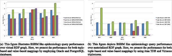
BSBM like epidemiology query performance over virtual and materialized RDF graphs
Fig. 11 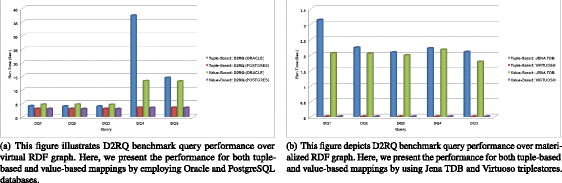
D2RQ benchmark query performance over virtual and materialized RDF graphs


The above observations show that queries that need multiple data sources to retrieve results perform better with the value-based approach. On the other hand, queries that need a single data source have approximately the same execution time regardless of which mapping was used. This is because tuple-based mapping ignores primary key and foreign key relationships, and converts all the relational database values to literals. This leads to the duplication of data in the RDF graph. Moreover, there is no explicit link between data entities exits in tuple-based mapping. Hence, complex queries that need numerous data sources to answer take a longer time to execute in RDF graphs constructed with the tuple-based mapping approach. However value-based mapping preserves primary key and foreign key relationships that link multiple data sources. Therefore, complex queries that need multiple datasets join to retrieve results that execute faster in RDF graph created with valued-based mapping approach. Hence, most of the queries mentioned in Table 9 execute faster with a RDF graph created with values-based mapping. However, most of the benchmark queries mentioned in Tables 10 and 11 do not need multiple data sources to retrieve the results. Hence their performance over RDF graphs constructed with tuple-based and value-based mappings are relatively similar. Note that the triplestores and the relational databases indexing algorithms have a significant impact on query performance. We use two different triplestores (Virtuoso and Jena TDB) and relational databases (Oracle and PostgreSQL) in our experiments. We find that that our query execution time depends on internal indexing algorithms used by the two systems. Moreover, query performance depends on the hardware configuration as well. These aspects will need to be taken into account before deploying the system as a part of a production system.
6 Analytics with EpiK
We briefly describe the kinds of analytics that can be done using EpiK. The goal is not to be exhaustive but to convey the utility of developing an environment such as EpiK. We describe three simple examples. The examples are chosen based on the following: (i) to illustrate the value of developing a federated data representation so that insights can be obtained by reasoning over multiple datasets simultaneously and (ii) to illustrate the use of SPARQL and RDF in terms of query language and data representation; this allows us to develop network queries that are pertinent in epidemic analysis; (iii) illustrate “realistic” studies that can be undertaken in the agent-based epidemic analysis. All the queries that arose in the examples below are done using the EpiK. In our experimentation, we use a materialized RDF graph generated through the value-based mapping approach. The materialized RDF graph is constructed from various datasets used and generated by one cell ten replicate influenza simulation study.
Example 1: Understanding the Structure of the Dendograms
A basic task in an epidemic analysis is to understand the structure of the dendogram. The dendogram is a directed acyclic graph (DAG), and one can also do basic analysis that involves the demographics of the infected individuals. We analyze ten dendograms coming from ten replicates. We compute basic properties of a dendogram: degree, path, and star distributions. We count distinct star patterns only and discard duplicates. For example, a five nodes star is not included in a six nodes star. However, duplication is considered in path counts. In our experimentation minimum star length is four nodes. The degree, star, and path distributions of the ten replicates are shown in Figs. 12, 13, and 14. Fig. 12 shows that we have few high degree nodes and many low degree nodes. Similarly, Figs. 13 and 14 show that we have a small amount of long path (or large star) and many small paths (or stars). Moreover, Figs. 12 and 14 show that replicates are relatively similar for degree and star distributes. Furthermore, the distributions contain long tails. However, it is not the case for path distribution. Figure 13 shows that replicates have variations and do not have the long tail like degree and star distributions. In Tables 16, 17, and 18, we provide detailed information of degree, path, and star counts. A summary statistics across all the replicates is presented in Table 19.

This figure shows degree distribution information of a ten replicates one cell experiment. For each replicate, we present node degree in the x-axis and fraction of nodes in the y-axis. The figure depicts that degree distributions for ten replicates are similar. We have a lower number of higher-degree nodes and a higher number of lower-degree nodes

This figure provides path distribution information. We count the number of occurrences of the various length of paths in the dendograms. Plots show the path length distribution across replicates is similar

This figure represents the distribution of the star patterns in the dendograms. We present star size (number of nodes in a star) in the x-axis and fraction of total stars in the y-axis
Example 2: Understanding Chains of Transmissions in Epidemics
During the course of H5N1 planning efforts, several groups including ours were interested in understanding long chains of epidemic transmission. The basic idea builds on Example 1 and tries to understand super-spreaders. In epidemiology discipline, it is important to identify super-spreaders because many disease distribution of infection rate infers that 20% of the population cause the 80% of the diseases spread [97]. Hence, super-spreader information can help policy makers to design precise interventions to effectively diminish the epidemic.
Intuitively, a node (individual) is a super-spreader if the node infects many other nodes. The basic issue of interest is direct infections versus indirect infections. A direct super-spreader is a node directly infects a large number of individuals. An indirect super-spreader is a node that is the root of long chain of infections. Intuitively, these two transmission pathways are different. The first resembles a star while the later is long path in the dendogram. Understanding the distribution of paths and stars in a dendogram thus provides us with an understanding of the transmission structure. An analysis across multiple dendograms tells us how robust the conclusions are within a single cell of the experiment (and thus provides a basis for sensitivity analysis). We present path and star distributions in Figs. 13 and 14 (count information in Tables 17 and 18). The figures clearly show a small number of occurrences of super-spreaders across different replicates. Policy makers can use this super-spreader information to design targeted interventions (e.g., vaccinations) to stop the disease propagation.
Example 3: Investigating the Role of School Children in Disease Transmission
As a final example, we study the role of school children in an epidemic. Intuitively, it is well accepted that school children play an important role in epdemics [98, 99]. EpiK can be used for a simulation-based analytical experiment to understand this. We look at dendograms produced by simulations as discussed in the earlier experiments. We look at two kinds of motifs. We look at paths of various lengths in which the starting node is a school-aged child (age range 3–18). We also look at stars of various sizes where the root of the star motif is a school-aged child. Our results are summarized in Figs. 15 and 16. In both the plots, for a given size S, the y-axis plots the percentage of the fraction \(\frac {A}{B}\) where A is the total number of paths (stars) of size S where the root is a school-aged child and B is the total number of paths (stars) of size S. The higher the fraction, the more prominent the role of a school-aged child. The figures clearly show that school-aged children play an important role in epidemic spread. For example, by examining Fig. 15 we see that for most of the path lengths, over 50% of the paths have a school-aged child as a root. The same conclusion folds for stars. Furthermore, for 100% of the large stars (sizes 9, 10, 21) and path’s (size 27) roots nodes (act as a super-spreader) are school-aged children.

The figure illustrates the percentage of the paths (over total) where root infector is a school child for various path lengths. We present path length in the x-axis and school child root infector paths percentage on the y-axis

In this figure, we show for several star size the percentage of star patterns (over total) where the root node is a school infected child. We present star size in the x-axis and school child root infector stars percentage on the y-axis. In the experiment, we consider four nodes as a minimum length of a star pattern
The choice of paths and stars is important. Stars represent a particular school-aged child infecting many other individuals in a small time frame; a path represents a school-aged child being the originator of a sustained transmission chain. Each motif points to a different role played by a school-aged child. The high fraction of such motifs with school-aged children as root provides evidence that school children play a major role in disease transmission.
This example illustrates how simulations can be used to assess the important role of school children in an epidemic spread. To do this, first we look at paths in which a single school kid infects many other individuals. Second, we look at all edges in the dendogram in which the infector node is a school age child and the infectee is any type (star pattern). We compute the total number of occurrences of various length of path and star patterns across all the replicates where the root node belongs to any demographic groups (school age, young age, middle age, and senior age). We also compute the total number of occurrences of various length of path and star patterns where the root node is a school infected child (age range 3–18) across all the replicates. We calculate the percentage of the different length of path and star patterns occurrences where the root node is a school infected child over all the replicates. We present path and star patterns percentage information in Figs. 15 and 16. Figure 15 shows that for various path lengths (1–27) over all the replicates most of the time more than 50% originator of a path infection is a school-infected child (except for path lengths 23, 24, and 26). Moreover, across all the replicates, 100% longest path’s (size 27) root node (act as a super-spreader) is a school-infected child. Similarly, Fig. 16 represents across all the replicates for various star size most of the time more than 50% root node of a star infection is a school-infected child (except for star size 8). Furthermore, 100% of the large size stars (size 9, 10, 21) roots nodes (act as a super-spreader) are school infected children (over all the replicates). Hence Figs. 15 and 16 support that more than half of the infection hosts and a significant number of super-spreaders are school-infected children.
The graph pattern queries (e.g., path, star) are crucial for understanding disease propagation and design of effective interventions. SIBEL system can be enhanced by using EpiK and the query bank described above. Currently, the SIBEL backend organizes the data using a RDB. As a part of future work, we will integrate EpiK and SIBEL. This will allow analysts to execute complex graphical queries. This will allow us to avoid expensive join operations and execute path and network motif style queries more efficiently. The queries described above capture a number of realistic scenarios that analysts using SIBEL encountered.
7 Concluding Remarks
We described a knowledge base (EpiK) to store, organize, integrate, and retrieve diverse and heterogeneous datasets occurring in the context of agent-based epidemiological modeling and analytics of infectious diseases. Our results demonstrate that epidemic analysis and data management can benefit from a knowledge base such as EpiK. Semantic web technologies played an important in the development of EpiK that provides a flexible mechanism for creating a federated data layer. EpiK is designed to accommodate the continued growth of output data. EpiK allows programmatic data access and execution of complex queries over datasets spanning the entire agent-based modeling workflow. The query bank provides examples of the kinds of analysis that can be done using EpiK. As users add new types of queries to the system, the task of an analyst can become progressively easier. To the best of our knowledge, this is the first attempt to develop a benchmark suite in this area. Finally, by running various epidemiologically relevant queries with two types of data mapping techniques, we demonstrate the performance of various tools. The empirical results show that our proposed framework is capable of extracting complex query results from heterogeneous data sources, with performance comparable to the state-of-the-art technologies.
We conclude with directions for future research. Our efforts have focused primarily on infectious disease epidemiology—extensions to chronic disease and environmental epidemiology would be interesting next steps. Extensions will also be needed when studying vector-borne and water-borne diseases to represent vectors, climatic, hydrological environmental, and ecological datasets. These extensions pose new challenges. We briefly discuss a few of them. Extension of EpiK to study infectious diseases such as Malaria and Zika require data pertaining to vectors, weather and the habitat of the vector. Weather, ecological and land cover datasets come from various sources and would need to be mapped on a common coordinate system. The World-pop and Malaria-Map projects [100,101,102] have begun important work in this direction. Coupling these efforts with modeling environments and analytics such as SIBEL will be useful in the design and analysis of public policies.
Notes
SIBEL was formerly called ISIS
References
Pyne S, Marathe MV, Vullikanti AKS (2015). In: Govindaraju V, Raghavan VV, Rao CR (eds) Big data applications in health sciences and epidemiology, handbook of statistics, volume 33: Big data analytics. Elsevier, Amsterdam
Marathe MV, Vullikanti AKS (2013) Computational epidemiology. Commun ACM 56(7):88–96
World Health Organization (WHO), http://www.who.int/topics/epidemiology/en/, [Online; accessed 2015-04-10]
Anderson RM, May RM (1991) Infectious diseases of humans. Oxford University Press, Oxford
Bailey NTJ (1975) The mathematical theory of infectious diseases and its applications. Hafner Press, New York
Hethcote HW (2000) The mathematics of infectious diseases. SIAM Rev 42:599–653
Salathe M, Bengtsson L, Bodnar TJ, Brewer DD, Brownstein JS, Buckee C, Campbell EM, Cattuto C, Khandelwal S, Mabry PL, et al. (2012) Digital epidemiology. PLoS Comput Biol 8(7):1–5
Chakraborty P, Khadivi P, Lewis B, Mahendiran A, Chen J, Butler P, Nsoesie EO, Mekaru SR, Brownstein JS, Marathe MV, et al. (2014) Forecasting a moving target: ensemble models for ILI case count predictions. In: Proceedings of the 2014 SIAM International Conference on Data Mining. Society for Industrial and Applied Mathematics, pp 262–270
Nsoesie EO, Brownstein JS, Ramakrishnan N, Marathe MV (2014) A systematic review of studies on forecasting the dynamics of influenza outbreaks. Influenza Other Respir Viruses 8(3):309–316
Zhang Q, Perra N, Perrotta D, Tizzoni M, Paolotti D, Vespignani A (2017) Forecasting seasonal influenza fusing digital indicators and a mechanistic disease model. In: Proceedings of the 26th International Conference on World Wide Web. International World Wide Web Conferences Steering Committee, pp 311–319
Eubank S, Guclu H, Kumar V, Marathe MV, Srinivasan A, Toroczkai Z, Wang N Modelling disease outbreaks in realistic urban social networks
Epstein JM (2009) Modelling to contain pandemics. Nature 460(7256):687–687
Lofgren E, Halloran ME, Rivers CM, Drake JM, Porco TC, Lewis B, Yang W, Vespignani A, Shaman J, Eisenberg JNS, Eisenberg MC, Marathe MV, Scarpino SV, Alexander KA, Meza R, Ferrari MJ, Hyman JM, Meyers LA, Eubank S (2014) Opinion: mathematical models: a key tool for outbreak response. PNAS 111:18095–18096
Kerkhove MV, Ferguson N (2012) Epidemic and intervention modelling–a scientific rationale for policy decisions? lessons from the 2009 influenza pandemic. Bull World Health Organ 90:306–310
Lipsitch M, et al. (2011) Improving the evidence base for decision making during a pandemic: the example of 2009 influenza-A H1N1 Biosecur Bioterror
Brauer F, van den Driessche P, Wu J (eds) (1945) Mathematical Epidemiology, ser. Springer, Berlin. Lecture Notes in Mathematics
Kaplan E, Craft D, Wein L (2002) Emergency response to a smallpox attack: the case for mass vaccination, PNAS
Keeling MJ, Eames KTD (2005) Networks and epidemic models. J R Soc Interface 2:295–307
Meyers LA, epidemiology Contact network (2007) Bond percolation applied to infectious disease prediction and control. Bull Am Math Soc 44:63–86
Gilbert N (2007) Agent-based models sage publications
Beckman R, Bisset K, Chen J, Lewis B, Marathe MV, Stretz P (2014) ISIS: A networked-epidemiology based pervasive Web app for infectious disease pandemic planning and response. In: Proceedings of the 20th ACM SIGKDD international conference on Knowledge discovery and data mining. ACM, pp 1847–1856
Grefenstette JJ, Brown ST, Rosenfeld R, DePasse J, Stone NT, Cooley PC, Wheaton WD, Fyshe A, Galloway DD, Sriram A, Guclu H, Abraham T, Burke DS (2013) FRED (A Framework for Reconstructing Epidemic Dynamics): an open-source software system for modeling infectious diseases and control strategies using census-based populations. BMC Public Health 13(1):1–14. [Online]. Available: https://doi.org/10.1186/1471-2458-13-940
Lopes LF, Silva FA, Couto F, Zamite J, Ferreira H, Sousa C, Silva MJ (2010) Epidemic marketplace: an information management system for epidemiological data. In: Information Technology in Bio-and Medical Informatics, ITBAM 2010. Springer, pp 31–44
CDC: Influenza (Flu), https://www.cdc.gov/flu/weekly/, [Online; accessed 2017-04-17]
HealthMap: Global Health, Local Information, http://www.healthmap.org/en/, [Online; accessed 2017-04-17]
Texas Pandemic Flu Toolkit, http://flu.tacc.utexas.edu/, [Online; accessed 2017-04-17]
LANL BARD, https://brd.bsvgateway.org/brd/, [Online; accessed 2017-04-17]
EpiC Framework, http://www.mobs-lab.org/, [Online; accessed 2017-04-17]
User Manual for DIDACTIC, 2009, http://ndssl.vbi.vt.edu/didactic/DidacticUserManual.pdf
Bisset K, Chen J, Feng X, Kumar V, Marathe MV (2009) EpiFast: a fast algorithm for large scale realistic epidemic simulations on distributed memory systems. In: Proceedings of the 23rd international conference on Supercomputing. ACM, pp 430–439
Barrett CL, Bisset K, Eubank S, Feng X, Marathe MV (2008) EpiSimdemics: an efficient algorithm for simulating the spread of infectious disease over large realistic social networks. In: Proceedings of the 2008 ACM/IEEE conference on Supercomputing. IEEE Press, pp 1–12
Pratt JM, Cohen M (1992) A process-oriented scientific database model. ACM SIGMOD Record 21(3):17–25
Pratt JM (1995) Data modeling of scientific experimentation. In: Proceedings of the 1995 ACM symposium on Applied computing. ACM, pp 86–90
Shi H, Zhang Y, Zhang J, Wan P, Shaw K (2007) Development of web-based epidemiological reporting system for tasmania utilizing a google maps add-on. In: 9th Biennial Conference of the Australian Pattern Recognition Society on Digital Image Computing Techniques and Applications. IEEE, pp 118–123
Allon D, Nicholson P Data Modelling for an Epidemiological Database. http://www.sascommunity.org/seugi/SEUGI1997/ALLON_POSTERS.PDF, 1997, [Online; accessed 2015-03-25]
Sequeda JF, Arenas M, Miranker DP (2012) On directly mapping relational databases to RDF and OWL. In: Proceedings of the 21st international conference on World Wide Web. ACM, pp 649–658
Bertails A, Prud’hommeaux EG (2011) Interpreting relational databases in the RDF domain. In: Proceedings of the sixth international conference on Knowledge capture. ACM, pp 129–136
Salas PE, Marx E, Mera A, Viterbo J (2011) RDB2RDF plugin: relational databases to RDF plugin for eclipse. In: Proceedings of the 1st Workshop on Developing Tools as Plug-ins. ACM, pp 28–31
Zappa A, Splendiani A, Romano P (2012) Towards linked open gene mutations data. BMC Bioinf 13(Suppl 4):S7
Dalamagas T, Bikakis N, Papastefanatos G, Stavrakas Y, Hatzigeorgiou AG (2012) Publishing life science data as linked open data: the case study of miRBase. In: Proceedings of the First International Workshop on Open Data. ACM, pp 70–77
Hert M, Reif G, Gall HC (2010) Updating relational data via sparql/update. In: Proceedings of the 2010 EDBT/ICDT Workshops. ACM, p 24
Piro R, Nenov Y, Motik B, Horrocks I, Hendler P, Kimberly S, Rossman M (2016) Semantic technologies for data analysis in health care. In: International Semantic Web Conference. Springer, pp 400–417
Horrocks I, Giese M, Kharlamov E, Waaler A (2016) Using semantic technology to tame the data variety challenge. IEEE Internet Comput 20(6):62–66
Bornea MA, Dolby J, Kementsietsidis A, Srinivas K, Dantressangle P, Udrea O, Bhattacharjee B (2013) Building an efficient RDF store over a relational database. In: Proceedings of the 2013 International Conference on Management of Data. ACM, pp 121–132
Groppe J, Groppe S, Ebers S, Linnemann V (2009) Efficient processing of SPARQL joins in memory by dynamically restricting triple patterns. In: Proceedings of the 2009 ACM symposium on Applied Computing. ACM, pp 1231–1238
Hert M, Reif G, Gall HC (2011) A comparison of RDB-to-RDF mapping languages. In: Proceedings of the 7th International Conference on Semantic Systems. ACM, pp 25–32
Arenas M, Grau BC, Kharlamov E, Marciuška Š, Zheleznyakov D (2016) Faceted search over RDF-based knowledge graphs. Web Semant Sci Serv Agents World Wide Web 37:55–74
Gupta S (2011) A unified data model and declarative query language for heterogenous life sciences data, San Diego Super Computing Center, UCSD, Tech. Rep. SDSC TR-2011-3
Birkland A, Yona G (2006) BIOZON: a system for unification, management and analysis of heterogeneous biological data. BMC Bioinf 7(1):70
Noy NF, Shah NH, Whetzel PL, Dai B, Dorf M, Griffith N, Jonquet C, Rubin DL, Storey M-A, Chute CG, et al. (2009) Bioportal: ontologies and integrated data resources at the click of a mouse. Nucleic Acids Res 37(suppl 2):W170–W173
Chen H, Wu Z, Zheng G, Mao Y (2004) RDF-based schema mediation for database grid. In: Fifth IEEE/ACM International Workshop on Grid Computing, 2004. Proceedings. IEEE, pp 456–460
Kamdar MR, Dumontier M (2015) An Ebola virus-centered knowledge base, Database: the journal of biological databases and curation 2015, pp bav049
Jordan TH. SCEC 2009 Annual Report, Southern California Earthquake Center, 2009. [Online]. Available: http://www.scec.org/aboutscec/documents/SCEC2009_report.pdf
Borgman CL, Wallis JC, Mayernik MS, Pepe A (2007) Drowning in data: digital library architecture to support scientific use of embedded sensor networks. In: Proceedings of the JCDL 2007. [Online]. Available: 10.1145/1255175.1255228, pp 269–277
Candela L, Castelli D, Pagano P (2009) D4Science: an e-infrastructure for supporting virtual research. In: Proceedings of IRCDL 2009 - 5th Italian Research Conference on Digital Libraries, pp 166–169
Barrett CL, Bisset K, Eubank S, Fox E, Ma Y, Marathe MV, Zhang X (2007) A scalable data management tool to support epidemiological modeling of large urban regions. In: Research and Advanced Technology for Digital Libraries, pp 546–548
Schriml LM, Arze C, Nadendla S, Ganapathy A, Felix V, Mahurkar A, Phillippy K, Gussman A, Angiuoli S, Ghedin E, et al. (2010) GeMIna, Genomic metadata for infectious agents, a geospatial surveillance pathogen database. Nucleic Acids Res 38(suppl 1):D754–D764
Vector-Borne Disease Network, https://www.vecnet.org, [Online; accessed 2015-03-25]
Leidig JP Epidemiology Experimentation and Simulation Management through Scientific Digital Libraries, Ph.D. dissertation
Apache Jena: TDB. https://jena.apache.org/documentation/tdb/, [Online; accessed 2015-10-04]
Virtuoso Open-Source Edition, 2014, http://www.openlinksw.com/dataspace/doc/dav/wiki/Main/
D2RQ: Accessing Relational Databases as Virtual RDF Graphs, 2012, http://d2rq.org/, [Online; accessed 2015-04-10]
Hasan S, Gupta S, Fox E, Bisset K, Marathe MV, et al. (2014) Data mapping framework in a digital library with computational epidemiology datasets. In: 2014 IEEE/ACM Joint Conference on Digital Libraries (JCDL). IEEE, pp 449–450
U.S. Census 2000. 5-Percent Public Use Microdata Sample Files. https://www.census.gov/census2000/PUMS5.html https://www.census.gov/census2000/PUMS5.html, [Online; accessed 2015-03-25]
Bisset K, Chen J, Feng X, Ma Y, Marathe MV (2010) Indemics: an interactive data intensive framework for high performance epidemic simulation, pp 233–242
Resource Description Framework, https://en.wikipedia.org/wiki/Resource_Description_Framework, [Online; accessed 2015-04-10]
Why RDF for Healthcare Interoperability – Part 2 of Yosemite Series, http://yosemiteproject.org/recorded-webinars/2015-2/why-rdf-for-healthcare-interoperability-part-2-of-yosemite-series/, [Online; accessed 2015-04-10]
Jupp S, Malone J, Bolleman J, Brandizi M, Davies M, Garcia L, Gaulton A, Gehant S, Laibe C, Redaschi N, et al. (2014) The EBI RDF platform: linked open data for the life sciences. Bioinformatics 30(9):1338–1339
Linked data - connect distributed data across the web, http://linkeddata.org/, [Online; accessed 2015-04-10]
Triple Stores vs Relational Databases, http://stackoverflow.com/questions/9159168/triple-stores-vs-relational-databases, [Online; accessed 2015-04-10]
Fuseki: serving RDF data over HTTP. https://jena.apache.org/documentation/serving_data/, [Online; accessed 2015-10-04]
Installation and Configuration of the Virtuoso Faceted Browser. http://virtuoso.openlinksw.com/dataspace/doc/dav/wiki/Main/VirtFacetBrowserInstallConfig, [Online; accessed 2015-10-04]
Silk - The Linked Data Integration Framework, http://silkframework.org/, [Online; accessed 2015-04-10]
WELKIN. http://simile.mit.edu/welkin/
Lausen G (2008). In: Christophides V, Collard M, Gutierrez C (eds) Relational Databases in RDF: Keys and Foreign Keys, ser. Lecture Notes in Computer Science, vol 5005. Springer, Berlin. [Online]. Available: 10.1007/978-3-540-70960-2_3
de Laborda CP, Conrad S (2005) Relational. OWL: a data and schema representation format based on OWL. In: Proceedings of the 2nd asia-pacific conference on conceptual modelling, vol 43. Australian Computer Society, Inc., pp 89–96
Nyulas C, O’Connor M, Tu S (2007) Datamaster–a plug-in for importing schemas and data from relational databases into protege. In: 10th International Protégé Conference, pp 15–18
Curino C, Orsi G, Panigati E, Tanca L (2009) Accessing and documenting relational databases through OWL ontologies. Flexible Query Answering Syst 5822:431–442
Fisher M, Dean M, Joiner G (2008) Use of OWL and SWRL for semantic relational database translation in OWLED (spring)
Korotkiy M, Top JL (2004) From relational data to rdfs models. In: ICWE. Springer, pp 430–434
Champin P-A, Houben G-J, Thiran P (2007) Cross: an owl wrapper for reasoning on relational databases. ER 4801:502–517
Bizer C, Seaborne A (2004) D2rq-treating non-rdf databases as virtual rdf graphs. In: Proceedings of the 3rd International Semantic Web Conference (ISWC2004), vol 2004. Springer
Byrne K (2008) Having triplets-holding cultural data as rdf. In: Proceedings of the ECDL 2008 Workshop on Information Access to Cultural Heritage
Spanos D-E, Stavrou P, Mitrou N (2012) Bringing relational databases into the semantic web: a survey. Semantic Web 3(2):169–209
Five Ws, https://en.wikipedia.org/wiki/Five_Ws, [Online; accessed 2016-10-20]
Dolog P, Durão FA, Jahn K, Lin Y, Peitersen DK (2011) Recommending open linked data in creativity sessions using web portals with collaborative real time environment. J UCS 17(12):1690–1709
Kim HS, Son JH, Lim GH, Suh IH (2010) Semantic robot memory store using 5W1H for service tasks. In: International Conference on Advanced Mechatronics, pp 579–584
Yoshioka T, Herman G, Yates J, Orlikowski W (2001) Genre taxonomy: a knowledge repository of communicative actions. ACM Transactions on Information Systems (TOIS) 19(4):431–456
Johannessen MR, Følstad A (2014) Political social media sites as public sphere A case study of the norwegian labour party. Commun Assoc Inf Syst 34 (56):1067–1096
Ikeda T, Okumura A, Muraki K (1998) Information classification and navigation based on 5W1H of the target information. In: Proceedings of the 36th Annual Meeting of the Association for Computational Linguistics and 17th International Conference on Computational Linguistics-Volume 1. Association for Computational Linguistics, pp 571–577
Berlin SPARQL Benchmark (BSBM). http://wifo5-03.informatik.uni-mannheim.de/bizer/berlinsparqlbenchmark/, [Online; accessed 2015-03-25]
Benchmarking D2RQ v0.2. http://wifo5-03.informatik.uni-mannheim.de/bizer/d2rq/benchmarks/, [Online; accessed 2015-03-25]
SPARQL Query Language for RDF, 2014, http://www.w3.org/TR/rdf-sparql-query/
Oracle Corporation, https://www.oracle.com/index.html, [Online; accessed 2015-04-10]
PostgreSQL: The world’s most advanced open source database, https://www.postgresql.org/, [Online; accessed 2015-04-10]
High-Performance Computing and Information Technology, https://www.bi.vt.edu/services/computational-core, [Online; accessed 2017-04-17]
Galvani AP, May RM (2005) Epidemiology: dimensions of superspreading. Nature 438(7066):293–295
Fumanelli L, Ajelli M, Merler S, Ferguson NM, Cauchemez S (2016) Model-based comprehensive analysis of school closure policies for mitigating influenza epidemics and pandemics. PLoS Comput Biol 12(1):1–15
Glass K, Barnes B (2007) How much would closing schools reduce transmission during an influenza pandemic?. Epidemiology 18(5):623–628
Kraemer MU, Hay SI, Pigott DM, Smith DL, Wint GW, Golding N (2016) Progress and challenges in infectious disease cartography. Trends Parasitol 32(1):19–29
Hay SI, Guerra CA, Gething PW, Patil AP, Tatem AJ, Noor AM, Kabaria CW, Manh BH, Elyazar IR, Brooker S, et al. (2009) A world malaria map: plasmodium falciparum endemicity in 2007. PLoS Med 6(3):0286–0302
Gaughan A, Stevens FR, Linard C, Patel NN, Tatem AJ (2015) Exploring nationally and regionally defined models for large area population mapping. Int J Digital Earth 8(12):989–1006
Acknowledgements
We thank members of the Network Dynamics and Simulation Science Laboratory, Biocomplexity Institute, Virginia Tech., for their comments and suggestions. We especially thank Dr. Sandeep Gupta for working very closely with us on a number of topics related to the paper and for providing useful suggestions that greatly improved the paper. This work has been partially supported by DTRA CNIMS & DTRA BSVE (contract number HDTRA1-11-D-0016-0005), NSF DIBBS (Grant ACI-1443054), NIH MIDAS (Grant 5U01GM070694), and NSF BIG DATA (Grant IIS-1633028). The U.S. Government is authorized to reproduce and distribute reprints for Governmental purposes notwithstanding any copyright annotation thereon.
This manuscript has been authored in part by UT-Battelle, LLC under Contract No. DE-AC05-00OR22725 with the U.S. Department of Energy. The U.S. Government retains and the publisher, by accepting the article for publication, acknowledges that the U.S. Government retains a non-exclusive, paid-up, irrevocable, world-wide license to publish or reproduce the published form of this manuscript, or allow others to do so, for U.S. Government purposes. The Department of Energy will provide public access to these results of federally sponsored research in accordance with the DOE Public Access Plan (http://energy.gov/downloads/doe-public-access-plan).
Author information
Authors and Affiliations
Corresponding author
Ethics declarations
Competing interests
The authors declare that they have no conflict of interest.
Appendices
Appendix A: Synthetic Input Data
Appendix B: Disease Manifestation and Intervention Data
Rights and permissions
About this article

Cite this article
Hasan, S., Fox, E.A., Bisset, K. et al. EpiK: A Knowledge Base for Epidemiological Modeling and Analytics of Infectious Diseases. J Healthc Inform Res 1, 260–303 (2017). https://doi.org/10.1007/s41666-017-0010-9
Received:
Revised:
Accepted:
Published:
Issue Date:
DOI: https://doi.org/10.1007/s41666-017-0010-9