
Abstract
Human beings solve problems in different granularity worlds and shift from one granularity world to another quickly. It reflects human beings’ intelligence in problem solving to some extent. In the era of big data, some new problems are emerging in real life. For example, traditional big data processing models always compute from raw data, failing to consider the granularity feature of human. Thus, they are hard to solve the 3 V characteristics of big data. Granular computing (GrC) combines the multi-granularity thinking pattern of human intelligence with problem solving mode to deal with big data. Based on the related notions and characteristics of GrC, this paper reviews the previous studies of GrC in three progressive levels: granularity optimization, granularity conversion and multi-granularity joint problem solving. Then we proposed the diagram for relationship among three basic modes of GrC. Furthermore, the feasibility of GrC for big data processing is analyzed. Some research prospects of granular computing are given.
1 Introduction
With the rapid development of IT, communication technology, as well as the digitization in various fields, large amounts of data are being generated every day in different fields (Labrinidis and Jagadish 2012), such as hospitals, factories, mines, government agencies, schools, social networking sites, e-commerce and so on. Compared with traditional data, big data often contains large amounts of unstructured data requiring real-time analysis. The growth of data brings opportunities in mining its hidden value with great challenges (Andrew and Erik 2012; Clifford 2008).
Due to the worldwide information technology revolution, almost all industries are facing big data problems (Wu et al. 2014). Especially, for such high speed and massive data containing various valued information, information technology researchers meet enormous challenges. Therefore, as traditional computing platforms and communication networks fail to meet the challenges of big data, new solutions concerning storage technologies, next-generation networks, processors, programming languages and computational models should be studied and developed.
An obvious characteristic of human intelligence is to deal with problems hierarchically. In other words, problems are usually analyzed in different granularity levels. Granularity is a concept to reflect detailed information. In a philosophical point of view, the idea of granularity exists in the process of cognition, measure, concept formation and reasoning for any object (Yao 2000; Livi and Sadeghian 2016; Xu and Wang 2016; Antonelli et al. 2016; Lingras et al. 2016). To recognize a problem, people usually start to analyze it in a coarse granularity, and gradually penetrate into finer granularity level. An understanding of the underlying principles of human problem solving may help to consciously apply these principles (Yao 2011; Pedrycz and Chen 2011). For example, in chip debugging, circuit engineers usually use a holistic approach to analyze the overall framework, and then conduct a detailed analysis of the testing parameters and each module’s circuit structure until the flawed device is found out at last. In big data mining, people always start from specific data and mine the general rules from the data through abstract and summary.
Granularity is originally a concept of physics, referring to the mean metric of the substantial particle size. Here, it is used as a measure of the amount of information to analyze and process data in the domain space from different hierarchy. It aims to figure the amount of information in different granularities (Pedrycz 2013). Gradual granulation method of perceptions counts in marvelous capabilities that human intrinsically possess (Pedrycz 2013). As the objects of processing, granules are any subsets, objects, clusters, and elements of a universe as they are drawn together by distinguishability, similarity, or functionality (Yao et al. 2013). Skowron generalized the concept of granules to include “functional elements” such as classifiers, agents and agents group (Skowron and Wasilewski 2011). GrC is a label of the family of any theories, methodologies, techniques and tools. It is an information processing theory for using “granules” to build an efficient computational model for dealing with problems (Loia et al. 2016). Especially, when problems are with uncertainty, Grc can solve them approximately (Bazan 2008). Wherein, in GrC, all such constructed and/or induced objects are called granules (Skowron et al. 2016a). The structure used for representing and interpreting a problem or a system is called a granular structure (Kreinovich 2016). Figure 1 shows the entire granular structure, Layer k represents the finest layer, and each dot represents the finest data. A wide range of applications benefited from Grc, such as feature selection (Min and Xu 2016), time series forecasting (Maciel et al. 2016).

The diagram of information granule, granularity layer, and granularity structure
In the light of extensive results from many fields (Yao 2016) that use various mechanisms of Grc, it is important to construct conceptual reviews to support granular computing to better solve problems. Generally speaking, traditional granular computing mechanisms solve problems by serial computing methods on a single granularity layer (that means computed on a single granularity layer each time). However, when the problem is complex, we are hard to solve it only on any single layer with the sense of coarser result or finer result, and we should decompose the problem into several sub tasks to compute it on granularity layers to meet the demand of time-limit constraints. Evolving from GrC, multi-granularity thinking is effective approaches to deal with complex problem. Multi-granularity computing (MGrC) emphasizes on jointly utilizing multiple levels of information granules in problem solving, instead of only one optimal granular layer (Wang et al. 2015). Therefore, Multi-granularity joint problem solving (MGrJS) is a valuable research direction in the future if we want to improve the quality and efficiency of solution. But building this mechanism is not easy. Luckily, deep learning as a successful example model of MGrJS has made significant progress in the many fields, so its idea provides an heuristic way for us in the perspective of GrC.
The remainder is organized as follows. The following section gives an introduction to the characteristics and relative analysis of four main granular computing models and three mechanisms of granular computing in problem solving, namely, granularity optimization, granularity conversion and multi-granularity joint problem solving. A detailed analysis of deep learning, one of the vogue researches focusing on machine learning, is given in the view of granular computing. The relationship among the basic mechanisms of GrC is given after reviewing traditional mechanisms of GrC. Furthermore, combined with deep learning, we proposed the schematic diagram of MGrJS and made a feasible analysis of five theoretical models (fuzzy set, rough set, cloud model, quotient space, deep learning) of MGrC to the three GrC mechanisms. Section 3 analyzes the feasibility of applying Grc to deal with big data problems. In Sect. 4, on the basis of the challenges brought by big data, some research prospects of granular computing are proposed. The paper is briefly summarized in Sect. 5.
2 Granular computing
Three basic mechanisms of granular computing: granularity optimization, granularity conversion, and multi-granularity joint problem solving, can be summarized from previous research works according to the way in which GrC is used to solve problem. The notion of the three basic mechanisms is a new perspective on GrC. Each of the three mechanisms has its particular type of problem to deal with. Granularity optimization means to choose the most suitable granular level of a domain for the multi-granular information/knowledge representation model (MGrR), on which the most efficient and satisfactory enough solution is generated. In granularity conversion, the working granularity layer will switch between adjective layers or jump to a higher or lower granular layer in accordance with the requirements of solving a problem. Multi-granularity joint problem solving means to take a problem-oriented MGrR as input jointly employ every layer of the MGrR and finally achieve a correct solution to the problem. Next, we first introduce the common granular models, and on the basis make an elaborate illustration about the above mentioned mechanisms.
2.1 Granular computing models
The idea of granulation is at the heart of any knowledge representation system (Dubois and Prade 2016). The purpose of granulation is to get the right granule from the raw data. The first step is to select a specific model and then conduct granulation according to the corresponding granularity expression. The granulation models mainly include: fuzzy set (Zadeh 1965), rough set (Pawlak 1982, 1992, quotient space (Zhang and Zhang 1992), cloud model (Li et al. 1995), etc. These four granular computing models describe the human ability to solve the problem from different granularities. They come with their own methodologies, relative granularity structure, comprehensive design framework and a large body of knowledge supporting analysis, design, and processing of constructs developed therein. Table 1 indicates the common features of the four granular computing models.
-
1.
Fuzzy set.
Fuzzy set theory was first proposed by Zadeh in (1965) in the literature. In this theory, an element always belongs to a certain set to some extent or belongs to several sets in varying degrees. It studies a kind of uncertainty of division caused by the intermediate transitivity of the differences of objects. This uncertainty is something inherent and gets rid of the duality (either this or that) of classical mathematics, so that the extension of concept has an ambiguity (both this and that). Fuzzy set defined as follows: A is a mapping that set X to [0,1] A:X → [0,1], x → A(x). Then A is a fuzzy set on X, and A(x) is called the membership function of fuzzy set A.
Theory of fuzzy information granulation (Zadeh 1979) (TFIG) based on the fuzzy set is an important granulation model, which is inspired by human granulation and information processing and is roots in mathematics. The point of departure in TFIG is the concept of a generalized constraint. Granule is characterized by the generalized constraint that is used to define it. The principal types of granules include possibilistic, veristic and probabilistic (Pawlak 1992). The principal modes of generalization in fuzzy information granulation theory can be mainly generalized to fuzzification; granulation and fuzzy granulation (Zadeh 1997; Mendel 2016).
-
2.
Rough set.
Rough set theory was first proposed by Pawlak in (1982) in the literature and it is another way to deal with uncertainty. It could process data objectively without the prior information and has been widely used in pattern recognition, knowledge discovery, image processing and other fields (Skowron et al. 2015). The main idea of rough set is to build a division in the universe of discourse according to the equivalence relation and get indistinguishable equivalence classes, thus forming an approximate space composed by granules with different granularities (Wang et al. 2009). In this approximation space, the vague boundary set is described by the upper and lower approximation sets, while the boundary set is described by crisp set. Those elements, unable to be determined (cannot be classified) under the existing knowledge are all assigned to the border domain; while if the granularity is coarse, the border domain is wide, and the border domain is narrow if the granularity is fine. As elements in the same group (equivalence class) are indistinguishable, the information processing can be performed by the equivalence classes.
-
3.
Quotient space.
Quotient space theory was first proposed by Chinese scholars Zhang and Zhang in the literature (1992), which is a model for solving the problem from different perspectives and shifting the focus of thinking onto different abstract level by the idea of granularity. Granularity conversion process mainly depends on the “no-solution preserving” property and quotient approach principle in quotient space principles (Zhang and Zhang 2003). That is, when the classification technique is used to discuss a problem in coarse-granularity world, if the problem has no solution, then the original problem in fine-granularity world has no solution (truth preserving property). If a proposition is true in two quotient spaces with coarse-granularity, then it is true that their corresponding quotient space combined by them (falsity preserving property). This could narrow the solving area and accelerate the solving progress because the coarse-granularity world is generally simpler than the original world. Additionally, quotient approach principle is built on the fidelity insurance false principle and quotient space chain, i.e., these theories are based on the structure.
Zhang presented fuzzy quotient space theory to combine with the idea of fuzzy mathematics, which turns out to be a great mathematical model and tool for GrC (Zhang and Zhang 2005). Different grain size corresponds to different threshold values of membership function in the quotient space, into which fuzzy equivalence relation has been introduced by fuzzy quotient space theory. To construct normalized isosceles distance function has been presented further by Zhang, which is both in hierarchical way and between different quotient spaces, rendering it ability of extending a fuzzy quotient space theory with arbitrary threshold (Zhang et al. 2008).
-
4.
Cloud model.
Cloud model theory was proposed by Li (1995). It achieves bidirectional transformation of the qualitative concept and quantitative data by the forward and backward cloud transformation. A qualitative concept C is expressed by numerical characteristics (Ex, En, He), wherein, Ex is the core of a concept, En denotes the granularity scale of the concept, and He denotes the uncertainty of the concept’s granularity. It better characterizes the bidirectional cognitive transformation process of intension and extension of a concept, revealing the randomness and fuzziness of objective entity (Li et al. 2009), as shown in Fig. 2. Since a concept definitely has the property of granularity, mapping of quantitative values to a suitable grain-sized qualitative concept is also the process of granularity optimization. Granulation with the cloud model is to use the backward cloud transformation to get the numerical characteristic set. \(\{ ({\text{Ex}}_{i} ,{\text{En}}_{i} ,{\text{He}}_{i} )\} ,\quad i = 1,2, \ldots ,N\), and it could reflect the qualitative concept of the data set, then the data is divided into N granules. For example, in reference (Ma et al. 2012), cloud model was used as granulated model for image segmentation, in essence, which is the granulation process based on backward cloud generator and each divided region corresponds to a granule. Inspired by the idea of MGrC, adaptive gaussian cloud transformation (A-GCT) algorithm based on the cloud model was proposed by Liu et al. (2013). As shown in Fig. 3, based on the definition of parameter concept clarity, A-GCT could generate multi-granularity concepts by clustering academicians in Chinese Academy of Engineering with regards to age, which is also the process of granularity conversion.
Fig. 2 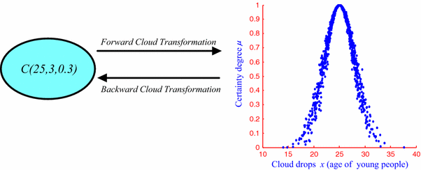
Bidirectional cognitive transformation of cloud model
Fig. 3 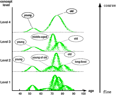
MGrR generated by A-GCT in the experiment of ACAE
In addition, there are some other granular computing models, cluster (Rodriguez and Laio 2014), shadowed sets (Pedrycz 1998), orthopairs (Ciucci 2016); they have common points with above mentioned models to manage uncertainty.


2.2 Granularity optimization
The purpose of granularity optimization is to seek the most suitable (the coarsest at sometime) granular layer of a domain for the MGrR, and the most efficient and satisfactory enough solution (meet the demand of time-limit constraints) is generated on this granular layer (Xu et al. 2015). The efficiency of the solution could be represented by solution effectiveness [GM (R), T] where R is the calculation result, GM (R) is the granularity of the solution and T is the time constraint. If the result granularity is expressed as GM (R u), and the time constraint is expressed as T u, granularity optimization is to find a certain granularity layer Layer i to meet GM(R i |R i = Solve(Layer i )) ≤ GM(R u) and T i ≤ T u. Then the intelligent calculation and analysis are implemented for the problem solving on the granularity level Layer i . As shown in Fig. 4, it shows the diagram of granularity optimization. Wherein, M PS is the mapping relation between problem granularity in leftmost part and the solution granularity, and M SC is the mapping relation between the solution granularity and computing granularity, and M PC is the mapping relation between problem granularity and computing granularity. Therefore, M PS and M SC could be used to obtain M PC. The granularity optimization algorithm is shown in the box, in essence, the solution mapped on Layer r could meet the granularity requirement but failed to meet the time constraint, while the solution mapped on Layer s could meet the time-limit constraint but its granularity is too coarse. The calculations on both granularity layers are all “invalid”. The solution mapped on Layer t could meet both the granularity requirement and the time-limit constraint, so the “valid” calculation is achieved by the granularity optimization.

Schematic diagram of granularity space optimization
In recent years, there are many researches on granularity optimization. Pedrycz (2011) and Pedrycz and Homenda (2013) proposed the principle of justifiable granularity, which combined the construction and optimization of information granularity. Zhang et al. (2015) combined the granularity space optimization and statistical probability theory to study the efficient multi-granularity search algorithm based on the statistical expectation, which analyzes the variation law of statistical probability expectation from the quotient spaces at different granularity levels and reduces the complexity to solve different probability models. Based on fuzzy compatibility relation, Wang et al. (2014) proposed a clustering granularity analysis method and it could determine the optimal clustering granularity by the synthesis and decomposition of fuzzy compatibility relation. Liu et al. (2014) proposed a granular computing classification algorithm based on distance measure and verified its superior accuracy by experiments. Bianchi et al. (2014) proposed a granular computing model to optimize pattern classification and found the optimal classification by this model. It has become a key point to design common pattern classification systems.
2.3 Granularity conversion
In essence, granularity conversion is to solve the problem by switching the working granularity layer between adjective layers or jump to a lower or higher granular layer, in accordance with the requirements of a problem. Granularity conversion means the same problem could be solved at different granularity layers. The key of granularity conversion is to study how to rapidly construct the solution on the adjacent granularity layer. The reconstruction mechanism based on the granularity conversion thinking pattern is shown in Fig. 5. Layer and Layer′ are two granularity layers and the problem could be solved by two ways, direct way and indirect way, represented by the red and blue arrow direction in Fig. 2. The direct way is to solve the problem directly by Layer′.

Fast solution reconstruction mechanism based on granularity conversion
The indirect way is to solve the mapping relation between solutions at different granularity layers in accordance with the relation between Layer and Layer′, and the solution of problem on Layer. Thus, for the Solution′
If we could first obtain the mapping relation f between solutions at different granularity layers t, then f is more effective than the only solution on Layer′. Wherein, h is determined by the layer granularity relation G and the problem on Layer. Therefore, we can achieve the fast reconstruction of adjacent granularity layers.
Researchers have done some meaningful works about granularity conversion. The quotient space proposed by Professor Zhang and Zhang (2003) is an earlier typical representative of granularity conversion. The original space is divided into spaces with different granularities, which is fully consistent with the equivalence relation in mathematics, then use the fidelity insurance false principle to select the most suitable elements from (X, F) to conduct problem solving. In addition, the relation between the elements of (X, F) is also obtained to explore the relation between solutions in the space with different granularities. It is a formal model to reflect human intelligence to solve problems. Based on a multi-layer granular structure, Yao and Luo (2011) proposed a top-down, step-wise progressive computing model and introduced a basic progressive computing algorithm to explore a sequence of refinements from coarser information granulation to finer information granulation. To make suitable assessments about students’ knowledge level, Collins et al. (1996) proposed a self-adaptive assessment system based on granularity layers and Bayesian network. Lin et al. (2014a, b) proposed a multi-granularity feature selection approach in emerging field. First, the neighborhood rough set was used as a granular computing tool to analyze the influence of neighborhood granularity, thus obtaining the feature ranking based on different granularity influence. Then, a new feature selection algorithm was born from the feature rankings. Wang et al. (2008) reviewed the uncertainty of rough set at different granularities and discussed the relation between roughness and ambiguity of the rough set under different knowledge granularities. As shown in Fig. 2, cloud model with A-GCT (Liu et al. 2013) algorithm is also an example of granularity conversion.
2.4 Multi-granularity joint problem solving
As shown in Fig. 6, it is the diagram showing the relationship among three basic modes of GrC. The input of traditional problem solving method is usually the data on a single particle layer, while the data and information on other granular layers are seldom considered. When the task is complex, it needs to integrate the solution components on each layer to form the right solution of the entire problem, and the input model of single granularity does not meet the needs of the solution. Therefore, the study of MGrJS includes two aspects: the construction and the multi-layer input of multi-layer problem solvers. Wherein, the construction of multi-layer problem solvers is crucial to multi-granularity computation. It should include the number of layers in multi-layer problem solvers, the establishment of the relationship between the layers and the structure of each layer, etc.

Diagram for relationship among three basic modes of GrC
The diagram of MGrJS is shown in Fig. 7. The essence of MGrJS is to utilize the multi-layer solvers to solve the problem based on the problem/field oriented granule structure. First, the task can be divided into subtasks with multiple granularities and each subtask corresponds to a layer-wise learner. Then, data with different granularities corresponding to multiple layer-wise solvers constitutes a granularity structure.

Schematic diagram of MGrJS
In recent years, deep learning (Hinton and Salakhutdinov 2006; Ranzato et al. 2015; Hinton et al. 2006; Salakhutdinov and Hinton 2009), as a successful model of MGrC, has made many significant progress in many fields, thus it become a hot topic in the field of machine learning. The success of deep learning is that it could solve a complex problem by dividing it onto many layers, and a relatively simple task is fulfilled on each single layer, which is essentially in accordance with the core idea of MGrC.
This idea of MGrJS can be traced back to some early research works in the 1990s. Jang and Roger (1993) proposed the fuzzy inference system (ANFIS) based on the adaptive network. It declared the birth of MGrJS. Figure 8 shows the structure diagram of ANFIS. It consists of five layers of neurons and three of them are hidden layers. In ANFIS, although each neuron could achieve different functions independently, they are interrelated on the whole, and could achieve fuzzy reasoning ultimately. The output expression is shown as follows:

ANFIS schematic diagram (Jang and Roger 1993)
Wang and Shi (1998) proposed the three-value/multi-value logic neural network TMLNN. This multi-layer neural network with neuron structure can express and cope with any three-value/multi-value logic problems. Figure 9 is an example that “exclusive or” is implemented by TMLNN.

TMLNN Schematic diagram (Wang and Shi 1998)
Deep learning was first proposed by Hinton et al. (2006). The idea of deep learning can be generalized as a model of solving problems by joint computing on multi-granularity information/knowledge representation (MGrIKR) in the perspective of Grc. It suggested that artificial neural network with multiple hidden layers has outstanding learning ability and could achieve more fundamental characterization from the data through learning. Thus, deep learning is suitable for visualization or classification. Difficulties in the training of deep neural network can be overcome by the layer-by-layer initialization.
Deep learning trains the presentation of the middle tiers using unsupervised learning and then abstract the high-level concepts by several lower-level components. Based on this feature, it achieved great success and has been widely applied in various fields such as visual perception (Zhou et al. 2015), object recognition (Mesnil et al. 2015), speech recognition (Han et al. 2014), etc. Currently, Tang’ research team achieve the highest precision in recognition of progress by far (Wang and Tang 2004; Cao et al. 2010; Luo et al. 2012; Sun et al. 2014). Especially, the DeepID face recognition technology developed by them could more accurate than the naked eye and the accuracy rate is over 99 %. As we know, LFW is the most widely used benchmarks in the face recognition field, and the deep learning model DeepID could obtain 99.15 % recognition rate on the LFW database. In addition, many other high-tech companies also invest a lot of resources in deep learning because they have seen that deep learning model plays a crucial role in mining the values of information in massive data in big data era, and could predict the future accurately.
In reference (Bengio et al. 2011), the deep learning was expounded as the structure shown in Fig. 10. If a certain learning algorithm acquired a good feature representation S 1 from the input data, it could be also used to get better feature representation S 2 from S 1, and so on. Based on the lower level feature, higher-level feature S i could be obtained by the non-linear transformation combination which has higher semantic expression and greater distinction degree.

Schematic diagram of deep learning (Bengio et al. 2011)
Figure 11 shows the deep Boltzmann machine (DBM) structure. Compared with the deep belief network, at each layer of DBM, the bottom-up approximate reasoning information with both-way junction could obtain the top-down feedback, thus the uncertainty of the input data can be well spread throughout the DBM network, so that the model is more robust. Because the supervised learning methods is used to initialize weights randomly and conduct fine tuning of DBM, these methods are likely to lead the network into a local minimum. The use of unsupervised pre-training methods is conducive to avoiding this problem (Erhan et al. 2010). In reference (Srivastava and Salakhutdinov 2014), combined with the common layer, two feature expressions of structure of learning text and image data were used, and it achieve the joint optimization of feature of two data sources.

Deep Boltzmann machine (Erhan et al. 2010)
Deep belief network (DBN) (Torralba et al. 2008) consists of restricted Boltzmann machine layers. This network is restricted as a visual layer and a hidden layer. The hidden layer units are trained to capture the coherence of high-level data manifested in visible layer. As shown in Fig. 12, v is the visible layer input of the first RBM and the generated hidden layer output h 1 is regarded as the visible layer input of the next RBM. h 1 is used to train new hidden layer output h 2. Then h 3 can be done by the same way. Convolutional neural networks (CNNs) (Krizhevsky et al. 2012; Liu et al. 2015) is one of the common models of deep learning and artificial neural networks. In 1984, Fukushima proposed a neocognitron (Fukushima 1980) based on the concept of receptive field (Hubel and Wiesel 1962) which could be regarded as the first implementing network of C. It is also the first application of the receptive field in artificial neural networks. CNNs is a multilayer perceptron to identify two-dimensional shape. This kind of network structure has high invariance property for translation, scaling, inclination or the transformation of common forms. As shown in Fig. 13, each layer of the CNNs includes several stages, like normalization, convolution, non-linear transformation, down-sampling, output features. The characteristic output of this layer is used as the input of next layer. The rest can be done by the same way. According to the actual application requirements, multiple similar processing stages could be added to extract multi-stage feature representation.

Deep belief network (Torralba et al. 2008)

Convolutional neural networks (Krizhevsky et al. 2012)
Deep learning has been successfully applied to a variety of classification problems, which will undoubtedly have an impact on machine learning and artificial intelligence systems. Andrew presented a new in-depth neural network permanent learning machines (PLMS) (Simpson 2015), overcoming some drawbacks of DNNs, especially the need for training before the use of DNNs. PLMS consists of two kinds of DNNs. One is called storage DNNs, used for classification of images, and the other is called recall DNN, used to generate new images. Bernardino put forward a new semantic segmentation algorithm (Zheng et al. 2015). Using the full convolution network plus a conditional random field as a recurrent neural network to conduct end to end training, it obtains a high accuracy. The machine vision project from the research teams of Yahoo lab has also made great achievements (Schifanella et al. 2015). Their goal is to find the hidden elements in images and features, such as emotion, society, esthetics, creativity and culture. For example, computer can predict the beauty of portrait by features and find the image features, such as the high correlation between contrast and sharpness with the senses and the low correlation between gender, age and race with the senses.
There are still a few differences between deep learning and MGrJS. The major differences between deep learning and MGrJS are that the input of deep learning is the finest-grained data while the input of MGrJS is MGrR, and the layer-wise learner of deep learning is usually a neural network while MGrJS’s layer-wise learner is any type of learning model.
Although there are some difference between deep learning and MGrJS, we can refer the idea of deep learning to study MGrJS basis on the above mentioned granulation models. The research should include decomposition mechanism of the problem, the partitioning mechanism of granularity and layers of different sub tasks, and the working mechanism of granular layer optimization, cross layer, and parallel computing. In short, MGrJS should be studied as one direction of GrC in the future.
The relationship among the three mechanisms and five theoretical models of MGrC is summarized in Table 2. Although we introduced fuzzy set and rough set in granularity optimization, and quotient space and cloud model in granularity conversion, it does not mean that the GrC models are limited to the corresponding mechanisms. Actually, fuzzy set and rough set can be used in granularity conversion, and quotient space and cloud model can be used in granularity optimization as well.
3 Big data and granular computing
As is well-known, big data has the 3 V characteristics, namely volume, velocity, variety (Clifford 2008).There are also different definitions. For example, the definition in IDC is that big data is to describe the new-generation technology and system architecture and then extract various economically valuable data through the acquisition, discovery or analysis (Gantz 2011). The 3 V characteristics indicate the significance and necessity of big data and also points out its core issue, how to tap the value from various and massive data with rapid growth.
Big data has brought new challenges (Chen and Zhang 2014; Du 2013; Tekiner and Keane 2013) for data computing in the data format, data analysis method, the timeliness and cost aspects of computing, etc. Many information technology researchers are seeking solutions from their own point of view. Figure 14 shows the diagram of big data processing, aiming to provide theoretical support for the application of big data from two aspects, big data processing paradigm and algorithm, and explore the related problems from its application and practice.

Diagram of big data processing
At present, there are various challenges in various stages brought by big data processing. The biggest problem is how to address the issues caused by 3 V features of big data. For example, in the phase of data acquisition, raw data not only includes the structured data, but also contains a lot of data with heterogeneity and uncertainty, so there are various problems to be solved, such as how to better access to standardization deterministic data; how to process big data with a huge scale and rapid growth and how to reduce the data scale and ensure its timeliness. In addition, data security issues are also to be considered, which means to make use of the big data and ensure that people’s privacy is not violated. Skowron et al. (2016b) pointed out that new challenges are to develop strategies to control, predict, and bound the behavior of the system based on big data at scale, and proposed to investigate these challenges using the GrC framework. Yao and Zhong (1999) argue that granular computing may have many potential applications in knowledge discovery and data mining, and analyzed connections of three related basic operations of granular computing (granulation of the universe, characterization of granules, and relationships between granules) to the tasks of knowledge discovery and data mining. Zhong et al. (2015) summarize the main aspects of brain informatics based big data interacting in the social-cyber-physical space of the Wisdom Web of Things (W2T). Yao (2000) pointed out that information granulation is to establish an effective user-centric concept based on the outside world and simplify our understanding of the physical world and the virtual world, which can efficiently provide practical inexact solution. Since this data processing computing model from the finest granularity fails to consider the actual grasp of granularity of human brain, this kind of raw data processing method is inconsistent with the law of human cognition. Peters and Weber (2016) proposed a framework—dynamic clustering cube (DCC) to categorize existing dynamic granular clustering algorithms, which motivate to use dynamic granular clustering in solving the velocity of big data. Therefore, multi-granularity thinking and problem solving mode of human intelligence could be used to build a new data processing computing model for big data.
In recent years, there are many already-existing industry examples of using granular optimization in big data processing. Slezak and Kowalski (2013) discussed how the specifics of data granulation methodology can affect the performance of Infobright database system. Synak and Slezak (2014) designed a new aggregation queries in Infobright database engine using the paradigms of rough sets and granular computing, which optimizes the decomposition of data blocks and aggregation groups among machines having access to shared data storage. Pai et al. (2015) proposed the implementation of computational intelligence including granular computing on air quality monitoring big data (AQMBD). Ryjov (2015) analyzed big data sources and made a conclusion that sizeable part of them is people-generated data, and present that how to make a choice the best (optimal) granulation.
Figure 15 is the frame of big data processing based on GrC. Three basic modes, including granularity optimization, granularity layer conversion and multi-granularity joint problem solving are used as the theoretical basis to support the entire big data processing. For some specific problems, it is necessary to consider information at multiple granularity levels. Three basic modes GrC mechanisms are beneficial to the process of the uncertainties, diversity, massiveness, and high speed access of big data. The steps are shown as follows: (1) data source selection and integration algorithms is adopted to conduct conversion, extraction, granulation for diverse and heterogeneous big data and then model for different heterogeneous data through different granularity data models. Then the granularity transformation is used to achieve conversion between uncertain information and certain information, thus obtaining the normalized big data. (2) Using the specific mode and thought of granular computing model to convert raw data into an appropriate granule and build corresponding granularity layer and structure. Establishing multi-granularity information knowledge representation model by the data in step (1). (3) Checking whether the raw data has the appropriate granularity and then providing feedback guidance for the raw data collection.

Frame of big data processing based on granular computing
4 Future research prospects of granular computing
Although some achievements have been achieved in GrC and big data processing, the applications of big data still needs to be improved. For example, how to effectively establish dynamic model for the multi-source heterogeneous big data and how to implement effective intelligent computing of big data, etc. Since we have solved these problems, now we can improve the ability of GrC to process big data.
-
1.
The unified structure of “from coarse to fine” and “from fine to coarse”.
Different problems require different granularity conversion mechanisms. If each sample is abstracted from the finest granularity, it could not meet the demand of time-limit constraints in the specific circumstances. So it is a good idea to combine the mechanism of “from coarse to fine” in our human with “from fine to coarse” in machine to build the unified structure to solve various problems.
-
2.
Human–machine progressive computing model.
Wilke and Portmann 2016 introduces a collaborative urban planning use case in a cognitive city environment and shows how an iterative process of user input and human oriented automated data processing can support collective decision making. Similarly, we proposed the prospects about two progressive computing models. First, it could solve problem by simulating the processes of human cognitive ability, through the coarsest granularity layer to get a global rough solution and then switch to finer layer according to the user constraints and time demand for further computation. Besides it also could solve problem by simulating the processes in automatic control, through the finest granularity layer to get a local temporary feasible solution and then switch to coarser layer for the global optimization computation, gradually to obtain the global optimal solution.
-
3.
The granulation of big data.
The granulation of big data is to conduct related researches on the characteristics such as mass, high speed. The traditional data analysis techniques based on database are always to carry out analysis and problem solving for the data with finest granularity and its data processing ability and speed cannot meet the needs of users in big data process. However, to conduct problem solving from the viewpoint of granular computing, granularity space corresponding to the problem could be selected. On this basis, granule with an appropriate granularity is regarded as the processing object, which could improve the efficiency of problem solving and obtain accurate solution. By building multi-granularity information knowledge representation model, the raw big data could be converted into small data without value loss, thus reducing the data scale and improve the quality and efficiency of problem solving of big data. As is well-known, some information granularity structures of big data are unknown and fixed, such as text. Others are unknown and varying, such as images, web internal structure. No matter they are fixed or varying, there are some problems like how to select basic elements from the information structure in the granulation process, how to conduct division, how to represent the structure between granularity layers and the interior structure of each layer, coupled with the uncertainty of the structure itself. To achieve the high speed and accelerate knowledge acquisition speed, a common approach is the incremental updating. Recently, incremental updating of rough set has made great achievement (Chen et al. 2011; Liang et al. 2014)
-
4.
Computing methods based on multi-granularity information and knowledge representation.
The computing methods based on the multi-granularity information and knowledge representation model of dynamic multi-source heterogeneous big data could be studied from two aspects. First, select any granularity layer in multi-granularity information and knowledge space to conduct problem solving and the solution on each layer has the same semantics, but the computing costs to obtain these solutions and their accuracy are different. Study the efficient computing method of variable granularity which could meet the time-limit constraints based on this kind of problem. Second, problem solving cannot be achieved at the same layer and it is necessary to combine multiple granularity layers. To solve this kind of problem, study the problem-oriented multi-granularity joint problem solving calculation method.
-
5.
Dynamic modeling and evolution mechanisms of multi-granularity information and knowledge space.
In the process of dynamic multi-source heterogeneous big data processing with the existing research methods, some problems are ignored, such as how to switch to an appropriate granularity to get the solution when the computing capability is insufficient or the time-limit constraints are satisfied. To meet the needs of real-time analysis, the current analysis methods of big data are limited by data type, data volume, data rate, computing power, and time-limit constraints which make them fail to provide an effective solution to meet customer needs in a timely manner. Therefore, it is necessary to study the dynamic modeling and evolutionary mechanisms of multi-granularity information knowledge space, including two aspects: the dynamic modeling around the granular computing and real-time dynamic evolution of granularity structure.
-
6.
Parallel granular computing of big data.
Based on the software platform and IT infrastructure, develop the acceleration in granular computing method analysis of big data by parallel computing. For those problems with mass data, high relevancy and weak parallelism, study the processing methods on open-source platform like Spark/Storm, Hadoop, etc. For the parallel compute-intensive tasks of data, study the computing cluster solution with high performance of GPU + CPU.
-
7.
Granular computing models in real life applications.
Combined with the specific application context, the big data processing method based on granular computing is used in scientific and engineering applications. For example, in aluminum electrolysis process industry, multi-granularity joint problem solving mechanism could be used to design knowledge automation aluminum electrolysis decision system based on big data, thus solve the relevant problems of decision-making system of modern aluminum electrolysis production. In the field of health care, based on the diagnosis and treatment data of different categories, we conduct multi-granularity joint problem solving for the complex task of big data and study how to explore the available information from medical data efficiently in several different scenarios like auxiliary monitor for the health care, public health surveillance and hospital decision-making management, so as to solve problems faced by the healthcare industry and make valuable decisions which could contribute to the society. In the field of ecological environment monitoring and early warning, with regard to the continuous physical and chemical process of water quality, we adopt multi-granularity modeling from different dimensions such as value of time, space and water quality to efficiently compute the water quality index of the specific location during the next period. These specific research works will continue to enrich the theoretical models and techniques of big data process based on the granular computing.
-
8.
Multi-granularity deep learning model.
There is a big gap between deep learning and human discriminating ability in target recognition of natural images and other applications. With the increasing size of data, it is necessary to adopt a more sophisticated model to capture richer information and patterns, which then requires higher computing capacity. The existing learning algorithms such as stochastic gradient descent, are serialized, so the key to improve the efficiency of model training lies in how to convert the asynchronous update mode into parallel computing model more effectively and take advantage of GPU parallel processing capability, etc.
-
9.
Deep learning theory support system.
Although a lot of achievements have been made in deep learning, these honored breakthroughs are based on experience and lack good theoretical support. Therefore, it is necessary to carry out further research and exploration to improve the theory and better guide the practice. Section 2.4 indicates that deep learning based on the multi-granularity joint problem solving is very powerful and could solve many practical problems, particularly in the field of dimensional reduction and genetic programming and other areas. However, the further study is still needed, for example, for a particular frame, the dimensions of input for optimum performance should be determined. Besides, a single deep learning approach cannot bring the best results and usually the combination of various methods for averaging scoring will bring a higher accuracy rate. Therefore, it is of great significance to study the integration of deep learning with other learning methods.
5 Conclusion
Although researches of Grc have been carried out for many years, previous studies mainly focus on the GrC model. To achieve the intelligent computing of big data with multi-granularity, it is necessary to study those basic problems with the data as the center, such as multi-granularity data expression and processing, multi-granularity intelligent computing model of big data, etc. Based on the previous works in three progressive levels: granularity optimization, granularity conversion and multi-granularity joint problem solving (MGrJS), this paper point out that MGrJS is a valuable research direction in the future if we want to improve the quality and efficiency of solution. We analyze the feasibility to apply the GrC to big data processing and emphasize that multi-granularity data processing model is an effective way to deal with the big data problems. Then we propose some suggestions for the future research, aiming to provide some valuable references and help for researchers engaged in granular computing and big data processing technique.
References
Andrew MA, Erik B (2012) Big data: the management revolution. Harv Bus Rev 90(10):60–6, 68, 128
Antonelli M, Ducange P, Lazzerini B et al (2016) Multi-objective evolutionary design of granular rule-based classifiers. Granul Comput 1(1):37–58
Bazan JG (2008) Hierarchical classifiers for complex spatio–temporal concepts. Transactions on rough sets IX. Springer, Berlin, pp 474–750
Bengio Y, Guyon G, Dror V et al (2011) Deep learning of representations for unsupervised and transfer learning. Workshop Unsuperv Transf Learn 7:17–37
Bianchi FM, Livi L, Rizzi A et al (2014) A granular computing approach to the design of optimized graph classification systems. Soft Comput 18(2):393–412
Cao Z, Yin Q, Tang X et al (2010) Face recognition with learning-based descriptor. IEEE Conf Comput Vis Pattern Recogn 6:2707–2714
Chen CLP, Zhang CY (2014) Data-intensive applications, challenges, techniques and technologies: a survey on big data. Inf Sci 275(11):314–347
Chen H, Li T, Ruan D et al (2011) A rough-set based incremental approach for updating approximations under dynamic maintenance environments. IEEE Trans Knowl Data Eng 25(99):1
Ciucci D (2016) Orthopairs and granular computing. Granul Comput 1(3):1–12
Clifford L (2008) Big data: how do your data grow? Nature 455(7209):28–29
Collins JA, Greer JE, Huang SX (1996) Adaptive assessment using granularity hierarchies and bayesian nets intelligent tutoring systems. Springer, Berlin, pp 569–577
Du Z (2013) Granularities and inconsistencies in big data analysis. Int J Software Eng Knowl Eng 23(6):887–893
Dubois D, Prade H (2016) Bridging gaps between several forms of granular computing. Granular Comput 1(2):115–126
Erhan D, Bengio Y, Courvulle A et al (2010) Why does unsupervised pre-training help deep learning? J Mach Learn Res 11(3):625–660
Fukushima K (1980) Neocognitron: a self-organizing neural network model for a mechanism of pattern recognition unaffected by shift in position. Biol Cybern 36(4):193–202
Gantz J, Reinsel D (2011) Extracting value from chaos, Idcemc2 Report
Han K, Yu D, Tashev I (2014) Speech emotion recognition using deep neural network and extreme learning machine. In: Interspeech, pp 223–227
Hinton GE, Salakhutdinov RR (2006) Reducing the dimensionality of data with neural networks. Science 313(5786):504–507
Hinton G, Osindero S, Teh Y (2006) A fast learning algorithm for deep belief nets. Neural Comput 18(7):1527–1554
Hubel DH, Wiesel TN (1962) Receptive fields, binocular interaction and functional architecture in the cat’s visual cortex. J Physiol 160(1):106–154
Jang RJS (1993) ANFIS: adaptive-network-based fuzzy inference systems. Inst Electr Electron Eng Inc 23(3):665–685
Kreinovich V (2016) Solving equations (and systems of equations) under uncertainty: how different practical problems lead to different mathematical and computational formulations. Granul Comput 1(3):1–9
Krizhevsky A, Sutskever I, Hinton GE (2012) ImageNet classification with deep convolutional neural networks. Adv Neural Inf Process Syst 25(2):2012
Labrinidis A, Jagadish HV (2012) Challenges and opportunities with big data. Proc VLDB Endow 5(12):2032–2033
Li DY, Meng HJ, Shi XM (1995) Membership clouds and membership cloud generators. J Comput Res Dev 32(6):15–20
Li DY, Liu CY, Gan WY (2009) A new cognitive model: cloud model. Int J Intell Syst 24:357–375
Liang JY, Wang F, Dang CY et al (2014) A group incremental approach to feature selection applying rough set technique. IEEE Trans Knowl Data Eng 26(2):294–308
Lin Y, Li J, Lin P et al (2014a) Feature selection via neighborhood multi-granulation fusion. Knowl Based Syst 67(3):162–168
Lin Y, Li J, Lin M et al (2014b) A new nearest neighbor classifier via fusing neighborhood information. Neurocomputing 143(16):164–169
Lingras P, Haider F, Triff M (2016) Granular meta-clustering based on hierarchical, network, and temporal connections. Granul Comput 1(1):71–92
Liu YC, Li DY, He W et al (2013) Granular computing based on Gaussian cloud transformation. Fundam Inf 127(14):385–398
Liu HB, Liu CH, Wu CG (2014) Granular computing classification algorithms based on distance measures between granules from the view of set. Comput Intell Neurosci 32(2):150–159
Liu JJ, Wang HX, Wang DS et al (2015) Parallelizing convolutional neural networks on intel many integrated core. architecture architecture of computing systems—ARCS 2015. Springer, Berlin, pp 71–82
Livi L, Sadeghian A (2016) Granular computing, computational intelligence, and the analysis of non-geometric input spaces. Granul Comput 1(1):13–30
Loia V, Aniello GD, Gaeta A, Orciuoli F (2016) Enforcing situation awareness with granular computing: a systematic overview and new perspectives. Granular Comput 1(2):127–143
Luo P, Wang X, Tang X (2012) Hierarchical face parsing via deep learning. Computer vision and pattern recognition (CVPR), 2012 IEEE Conference on. IEEE:2480–2487
Ma HY, Wang GY, Zhang QH (2012) Multi-granularity color image segmentation based on cloud model. Comput Eng 38(20):184–187
Maciel Leandro, Ballini Rosangela, Gomide Fernando (2016) Evolving granular analytics for interval time series forecasting[J]. Granul Comput 1(4):1–12
Mendel JM (2016) A comparison of three approaches for estimating (synthesizing) an interval type-2 fuzzy set model of a linguistic term for computing with words. Granul Comput 1(1):59–69
Mesnil G, Rifai S, Bordes A et al (2015) Unsupervised learning of semantics of object detections for scene categorization. Pattern recognition applications and methods, vol 318. Springer, Berlin, pp 209–224
Min F, Xu J (2016) Semi-greedy heuristics for feature selection with test cost constraints. Granul Comput 1(3):1–13
Pai TY, Chang MB, Chen SW (2015) Information granularity, big data, and computational intelligence. In: Pedrycz W, Shyi-Ming C (eds) Studies in big data, vol 8, pp 427–441
Pawlak Z (1982) Rough sets. Int J Comput Inform Sci 11(5):341–356
Pawlak Z (1992) Rough sets: theoretical aspects of reasoning about data. Kluwer Academic Publishers, Dordrecht
Pedrycz W (1998) Shadowed sets: representing and processing fuzzy sets. IEEE Trans Syst Man Cybern Part B Cybern A Publ IEEE Syst Man Cybern Soc 28(1):103–109
Pedrycz W (2011) The principle of justifiable granularity and an optimization of information granularity allocation as fundamentals of granular computing. J Inf Process Syst 7(7):397–412
Pedrycz W (2013) Granular computing: analysis and design of intelligent systems. CRC Press, Boca Raton
Pedrycz W, Chen SM (2011) Granular computing and intelligent systems: design with information granules of higher order and higher type. Springer, Berlin
Pedrycz W, Homenda W (2013) Building the fundamentals of granular computing: a principle of justifiable granularity. Appl Soft Comput 13(10):4209–4218
Peters G, Weber R (2016) DCC: a framework for dynamic granular clustering. Granul Comput 1(1):1–11
Ranzato M, Hinton G, Lecun Y (2015) Guest editorial: deep learning. Int J Comput Vis 113(1):1–2
Rodriguez A, Laio A (2014) Machine learning. Clustering by fast search and find of density peaks. Science 344(6191):1492–1496
Ryjov A (2015) Towards an optimal task-driven information granulation. information granularity, big data, and computational intelligence. Springer, Berlin, pp 191–208
Salakhutdinov Ruslan, Hinton Geoffrey (2009) Deep Boltzmann machines. J Mach Learn Res 24(5):448–455
Schifanella R, Redi M, Aiello L (2015) An image is worth more than a thousand favorites: surfacing the hidden beauty of Flickr pictures. arXiv:1505.03358 (preprint)
Simpson AJR (2015) On-the-fly learning in a perpetual learning machine. arXiv:1509.00913 (preprint)
Skowron A, Wasilewski P (2011) Information systems in modeling interactive computations on granules. Theoret Comput Sci 412:5939–5959
Skowron A, Jankowski A, Swiniarski RW (2015) Foundations of rough sets. In: Kacprzyk J, Pedrycz W (eds) Springer handbook of computational intelligence. Springer, Berlin, pp 331–348
Skowron A, Jankowski A, Dutta S (2016a) Interactive granular computing. Granul Comput 1(2):1–19
Skowron A, Jankowski A, Dutta S (2016b) Toward problem solving support based on big data and domain knowledge: interactive granular computing and adaptive judgement. Big data analysis: new algorithms for a new society. Springer, Berlin, pp 424–430
Slezak D, Kowalski M (2013) Intelligent granulation of machine-generated data. IFSA world congress and NAFIPS annual meeting (IFSA/NAFIPS), 2013 joint. IEEE, pp 68–73
Srivastava N, Salakhutdinov R (2014) Multimodal learning with deep boltzmann machines. J Mach Learn Res 15(8):1967–2006
Sun Y, Wang X, Tang X (2014). Deep learning face representation by joint identification-verification. In: International Conference on Neural Information Processing Systems. MIT Press, Cambridge, pp 1988–1996
Synak P, Slezak D (2014) Complexity aspects of multi-machine aggregations in a rough-granular computation framework. Granular computing (GrC), 2014 IEEE international conference on. IEEE, pp 275–280
Tekiner F, Keane JA (2013) big data framework. systems, man, and cybernetics (SMC), 2013 IEEE international conference on. IEEE, pp 1494–1499
Torralba A, Fergus R, Weiss Y (2008) Small codes and large image databases for recognition. 2008 IEEE conference on computer vision and pattern recognition. IEEE:1–8
Wang G, Shi H (1998) TMLNN: triple-valued or multiple-valued logic neural network. IEEE Trans Neural Netw 9(6):1099–1117
Wang XG, Tang X (2004) A unified framework for subspace face recognition. IEEE Trans Pattern Anal Mach Intell 26(9):1222–1228
Wang GY, Zhang QH et al (2008) Uncertainty of rough sets in different knowledge granularities. Chin J Comput 31(9):1588–1598
Wang GY, Yao YY, Yu H (2009) A survey on rough set theory and applications. Chin J Comput 32(7):1229–1246
Wang LW, Zhang XJ, Zhang L (2014) Cluster size analysis based on fuzzy compatibility relation. J Syst 26(7):321–329
Wang Guoyin, Ji Xu, Zhang Qinghua et al (2015) Multi-granularity intelligent information processing[J]. J Stroke Cerebrovasc Dis 2(1):S4–S5
Wilke G, Portmann E (2016) Granular computing as a basis of human–data interaction: a cognitive cities use case. Granul Comput 1(3):1–17
Wu XD, Zhu XQ, Wu GQ et al (2014) Data mining with big data. IEEE Trans Knowl Data Eng 26(1):97–107
Xu Z, Wang H (2016) Managing multi-granularity linguistic information in qualitative group decision making: an overview. Granul Comput 1(1):21–35
Xu J, Wang GY, Yu H (2015) Review of big data processing based on granular computing. Chin J Comput 8:1497–1517
Yao YY (2000) Granular computing: basic issues and possible solutions. In: Proceedings of the 5th joint conference on information sciences, vol I. Atlantic, NJ: Association for Intelligent Machinery, pp 186–189
Yao YY (2011) Artificial intelligence perspectives on granular computing. Granular computing and intelligent systems. Springer, Berlin, pp 17–34
Yao Y (2016) A triarchic theory of granular computing. Granul Comput 1(2):1–13
Yao YY, Luo J (2011) Top-down progressive computing. In: Proceedings of the 6th international conference on rough sets and knowledge technology. Springer, Berlin, pp 734–742
Yao YY, Zhong N (1999) Potential applications of granular computing in knowledge discovery and data mining. In: Proceedings of world multiconference on systemics, cybernetics and informatics, vol 5
Yao J, Vasilakos A, Pedrycz W (2013) Granular computing: perspectives and challenges. IEEE Trans Cybern 43:1977–1989
Zadeh LA (1965) Fuzzy sets. Inf Control 8(65):338–353
Zadeh LA (1979) Fuzzy sets and information granulation. Advances in fuzzy set theory and applications. North-Holland Publishing, Amsterdam
Zadeh LA (1997) Toward a theory of fuzzy information Granulation and its centrality in human reasoning and fuzzy logic. Fuzzy Sets Syst 90(2):111–127
Zhang B, Zhang L (1992) Theory and applications of problem solving. Elsevier Science Inc, Oxford
Zhang L, Zhang B (2003) The quotient space theory of problem solving. Fundam Inf 59(2):11–15
Zhang L, Zhang B (2005) Fuzzy reasoning model under quotient space structure. Inf Sci 173(4):353–364
Zhang QH, Wang GY, Liu XQ (2008) School of Information Science and Technology, University S J, Chengdu. Hierarchical structure analysis of fuzzy quotient space. Pattern Recogn Artif Intell
Zhang QH, Guo YL, Xue YB (2015) Multi-granularity search algorithm based on probability statistics. Pattern Recog Artif Intell 28(5):422–427
Zheng S, Jayasumana S, Romera-Paredes B et al (2015) Conditional random fields as recurrent neural networks. arXiv:1502.03240 (preprint)
Zhong N, Yau SS, Ma J et al (2015) Brain informatics-based big data and the wisdom web of things. IEEE Intell Syst 30(5):2–7
Zhou B, Garcia AL, Xiao J et al (2015) Learning deep features for scene recognition using places database. Adv Neural Inf Process Syst 1:487–495
Acknowledgments
This work is supported by the National Science Foundation of China (Nos. 61572091 and 61272060).
Author information
Authors and Affiliations
Corresponding author
Rights and permissions
About this article

Cite this article
Wang, G., Yang, J. & Xu, J. Granular computing: from granularity optimization to multi-granularity joint problem solving. Granul. Comput. 2, 105–120 (2017). https://doi.org/10.1007/s41066-016-0032-3
Received:
Accepted:
Published:
Issue Date:
DOI: https://doi.org/10.1007/s41066-016-0032-3