How do federal regulations affect consumer prices? An analysis of the regressive effects of regulation

Abstract

This study is the first to measure the impact of federal regulations on consumer prices. By combining consumer expenditure and pricing data from the Bureau of Labor Statistics, industry supply-chain data from the Bureau of Economic Analysis, and industry-specific regulation information from the Mercatus Center’s RegData database, we determine that regulations promote higher consumer prices, and that these price increases have a disproportionately negative effect on low-income households. Specifically, we find that the poorest households spend larger proportions of their incomes on heavily regulated goods and services prone to sharp price increases. While the literature explores other specific costs of regulation, noting that higher consumer prices are a probable consequence of heavy regulation, this study is the first to provide a thorough empirical analysis of that relationship across industries. Irrespective of the reasons for imposing new regulations, these results demonstrate that in the aggregate, the negative consequences are significant, especially for the most vulnerable households.

Appendices

Appendix 1: Proofs of predictions from theoretical model

Proof of Prediction 1

Consumer i’s spending on the regulated commodity as a share of her income is:

$$S_{i} = \frac{{px_{i} (p,m_{i} )}}{{m_{i} }}$$

(7)

Therefore:

$$\ln (S_{i} ) = \ln (p) + \ln (x_{i} (p,m_{i} )) - \ln (m_{i} )$$

(8)

$$\frac{{\partial \ln (S_{i} )}}{{\partial m_{i} }} = \frac{1}{{x_{i} }}\frac{{\partial x_{i} (p,m_{i} )}}{{\partial m_{i} }} - \frac{1}{{m_{i} }} = \frac{1}{{m_{i} }}\left[ {\varepsilon_{m} - 1} \right]$$

(9)

where $\varepsilon_{m}$ is the income elasticity of demand. Therefore, if demand with respect to income is inelastic, i.e., $0 < \varepsilon_{m} < 1$, then ${{\partial \ln (S_{i} )} \mathord{\left/ {\vphantom {{\partial \ln (S_{i} )} {\partial m_{i} }}} \right. \kern-0pt} {\partial m_{i} }} < 0$ □

Proof of Prediction 2

Application of the Implicit Function Theorem to Eq. (1) yields:

$$\frac{\partial p}{\partial R} = \frac{{\frac{\partial x(p,R)}{\partial R}}}{{\sum\nolimits_{i} {\frac{{\partial x_{i} (p,m_{i} )}}{\partial p} - \frac{\partial x(p,R)}{\partial p}} }} > 0$$

(10)

which shows that p is increasing in R. □

Proof of Prediction 3

Consumer i’s budget constraint is:

$$px_{i} (p,m_{i} ) + y_{i} = m_{i}$$

(11)

where y_i denotes consumer i’s expenditure on all commodities other than x_i. Dividing the budget constraint by m_i yields:

$$\frac{{px_{i} (p,m_{i} )}}{{m_{i} }} + \frac{{y_{i} }}{{m_{i} }} = 1$$

(12)

and differentiating with respect to R yields:

$$\frac{{x_{i} }}{{m_{i} }}\frac{\partial p}{\partial R} + \frac{p}{{m_{i} }}\frac{{\partial x_{i} (p,m_{i} )}}{\partial p}\frac{\partial p}{\partial R} + \frac{1}{{m_{i} }}\frac{{\partial y_{i} }}{\partial p}\frac{\partial p}{\partial R} = 0$$

(13)

Recall ${{\partial p} \mathord{\left/ {\vphantom {{\partial p} {\partial R}}} \right. \kern-0pt} {\partial R}} > 0$ that (Prediction 2). Equation (13) can be simplified to:

$$\frac{1}{{m_{i} }}\frac{{\partial y_{i} }}{\partial p} = - \frac{{x_{i} }}{{m_{i} }}\left[ {1 + \varepsilon_{p} } \right]$$

(14)

where is the regulated commodity’s price elasticity of demand. The left-hand side of Eq. (14) shows the proportional change in consumer i’s spending on other commodities when p increases. Recall that ${{x_{i} } \mathord{\left/ {\vphantom {{x_{i} } {m_{i} }}} \right. \kern-0pt} {m_{i} }}$ is decreasing in $m_{i}$ if demand with respect to income is inelastic (Prediction 1). Therefore, if demand with respect to price is also inelastic, i.e.,$- 1 < \varepsilon_{p} < 0,$ then an increase in p causes lower-income consumers to reduce their spending on other commodities by proportionately more than it does for higher-income consumers. □

Appendix 2: methodological description of the construction of the consumer expenditure survey and regulation datasets

To determine the disparate effects of government regulations on households in different socioeconomic strata, we construct a dataset that maps goods and services from the Consumer Expenditure Survey (CE) onto industry regulations from the Mercatus Center at George Mason University’s industry regulation database (RegData).

The CE provides detailed household spending and price data for a wide array of goods and services by income group. These goods and services are organized using the Universal Classification Codes (UCC) system. RegData 2.0, however, reports the level of industry regulation by the two-, three-, and four-digit North American Industry Classification System (NAICS) code for each year between 1997 and 2012. Therefore, to construct a usable database, we map regulations from the NAICS space onto goods and services in the UCC space. The resulting balanced panel dataset contains 9872 observations, covering 617 UCC-based goods and services over a 16-year period.

To construct the final dataset, the following steps are employed:

• 1. The RegData 2.0 dataset consists of two-digit, three-digit, and four-digit NAICS-based tables. Each regulation record in the tables contains the name of the government agency imposing the regulation, the year of the regulation, the industry affected by the regulation, the regulatory word count, the restriction count, and the industry regulation index value. For our purposes, we use the industry regulation index value, which equals the regulatory restriction count weighted by industry relevance.³¹

  For each industry-and-year pair, the industry regulation index values are summed across federal regulators. Therefore, for each industry-and-year combination, a single-industry regulation index value is derived, equaling the sum of all regulatory restrictions (weighted by industry relevance) imposed on that industry by all federal regulators for that year. The result is three aggregated datasets, one for each two-digit, three-digit, and four-digit NAICS-based table. Last, the three aggregated datasets are combined (stacked) to form a single dataset.

• 2. The spreadsheet containing the 2007 commodity-by-industry direct requirements (after redefinitions) table was downloaded from the Bureau of Economic Analysis (BEA) website (http://www.bea.gov/industry/xls/io-annual/CxI_DR_2007_detail.xlsx). This spreadsheet contains two work sheets, both of which are used below:

  • a. The first work sheet is a concordance that converts the BEA’s input–output (I–O) commodity/industry codes into 2007 NAICS codes.

  • b. The second work sheet is the I–O direct requirements table, which contains I–O weights ($\alpha_{ij}$) equal to the amount of input (measured in dollars) from industry ($i$) required to produce a dollar’s worth of output by industry ($j$). By construction, these weights sum to 1 because, in addition to actual inputs, the BEA includes employee compensation, taxes, and gross operating surplus in the weighting schema.

• 3. The I–O commodity/industry code to NAICS concordance described in step (2a) above is matched with the aggregate industry regulations from step (1), to create a new table that lists the aggregate industry regulations by I–O commodity/industry code; the resulting table is further summed over commodity code by year to derive a table with a single total regulation value for each commodity code–year pair. This second round of aggregation after the initial match is necessary because some commodity codes map onto multiple NAICS industries. I–O commodity/industry codes with no associated regulations are assigned an industry regulation index value of 0. The resulting table is a measure of the direct regulations (denoted $DirectReg_{it}$) applicable to a given I–O commodity/industry code.

• 4. To determine the level of regulation that applies to the inputs/supply chain of a given industry, the I–O direct requirements ($\alpha_{ij}$) from step (2b) are matched with the direct regulations for each I–O commodity ($DirectReg_{it}$) from step (3) by way of their I–O commodity/industry codes. Note that if a commodity/industry is not needed to produce a given output, the associated input value is 0. This produces a large result set with more than 2.4 million rows of data. This dataset is then “grouped by” output industry ($j$) and year ($t$) and summed over the product of the direct input regulations (indexed by i) and I–O weights, producing an estimate of input–supply chain regulation:$InputReg_{jt} = \mathop \sum \limits_{i} \alpha_{ij} \cdot DirectReg_{it} .$

  See Figure 4 for a graphical summary of steps (1) to (4).

  Fig. 4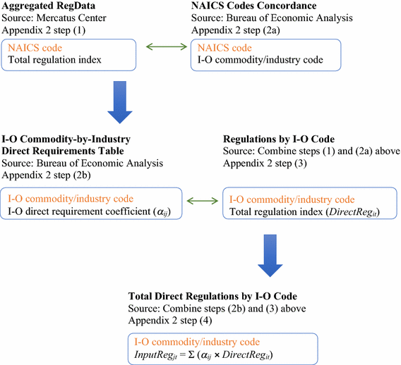

  

  Mapping regulations onto input–output (I–O) codes. Note: NAICS = North American Industry Classification System

• 5. The direct regulations by industry and year are matched with the total input regulations by industry and year. The direct and input regulations are summed to determine the total direct and indirect regulations affecting a given industry: $TotalReg_{it} = DirectReg_{it} + InputReg_{it} .$

• 6. To map regulations onto the UCC codes, a separate set of queries is executed to map the codes onto I–O commodity/industry codes.

  • a. As a beginning step, we import the personal consumption expenditures (PCE) concordance from the Bureau of Labor Statistics (BLS) (http://www.bls.gov/cex/pce_concordance_2012.xlsx) This file maps UCC codes onto PCE codes from the BEA’s national income and product accounts (NIPAs).

  • b. Next, we import BEA table 2.4.5U (I–O, Personal Consumption Expenditures by Type of Product with 2007 Input–Output Commodity Composition). This latter bridge file (http://www.bea.gov/national/xls/2007-pcs-io-bridge.xls) maps NIPA line numbers onto PCE codes.

  • c. The tables from steps (6a) and (6b) are matched by way of their common PCE codes. The resulting table serves as a bridge file that maps UCC codes onto NIPA line numbers.

• 7. Finally, we import the BEA’s PCE bridge file, which maps NIPA line numbers onto I–O commodity/industry codes (www.bea.gov/industry/xls/io-annual/PCEBridge_2007_Detail.xlsx), along with the total value of all purchases of the linked I–O commodity/industry in 2007.

  • a. Matching the NIPA line items from the PCE bridge with the results from step (6c) provides a clear mapping from UCC code to I–O commodity/industry codes. See Figure 5 for a graphic summary of steps (6) and (7).

    Fig. 5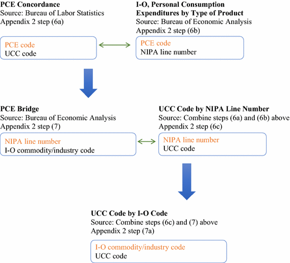

    

    Mapping input–output (I–O) codes onto consumer expenditure codes. Note: PCE = personal consumption expenditures; UCC = Universal Classification Codes; NIPA = national income and products accounts

• 8. The resulting table from step (7a) maps a given consumer product from the CE onto all I–O industries that produce that product. In many cases, more than one industry produces a given UCC product. To produce a single regulation value for each consumer product, we derive industry weights equal to a given industry’s 2007 level of output relative to the total output of all industries that supply a given UCC product.³² For example, the UCC code for flour is 10,110. This consumer product is produced by seven I–O industries. Assigning each of these industries a weight equal to its total output relative to the total output of all seven industries produces a set of weights that sum to 1 (see Table 8). Although it would be preferable to update these weights annually, the BLS derives these output data from the US Census Bureau’s Economic Census, which is conducted only every five years.

  Table 8 Input–output industries that produce flour (UCC: 10110)

• 9. Finally, UCC codes, I–O commodity/industry codes, and output shares from step (8) are matched with the regulation-by-industry data from step (5). These matched data are then “grouped by” UCC code and year and aggregated over the product of industry regulation and output shares.

See Table 9.

Table 9 Top 20 expenditure categories by income quintile and corresponding regulations

References

Al-Ubaydli, O., & McLaughlin, P. A. (2015). RegData: A numerical database on industry-specific regulations for all United States industries and federal regulations, 1997–2012”. Regulation & Governance. doi:10.1111/rego.12107.
Anderson, T. W., & Hsiao, C. (1982). Formulation and estimation of dynamic models using panel data. Journal of Econometrics, 18, 47–82.
Ardagna, S., & Lusardi, A. (2010). Heterogeneity in the effect of regulation on entrepreneurship and entry size. Journal of the European Economic Association, 8, 594–605.
Arellano, M., & Bond, S. (1991). Some tests of specification for panel data: monte carlo evidence and an application to employment equations. The Review of Economic Studies, 58, 277–297.
Becker, R. A. (2003). Pollution abatement expenditure by US manufacturing plants: Do community characteristics matter? B.E. Journal of Economic Analysis & Policy, 3, 1–23.
Becker, R. A., & Henderson, J. V. (2000). Effects of air quality regulations on polluting industries. Journal of Political Economy, 108, 379–421.
Becker, R. A., & Henderson, J. V. (2001). Costs of air quality regulation. In Carlo Carraro & Gilbert E. Metcalf (Eds.), Behavioral and distributional effects of environmental policy (pp. 159–168). Chicago: University of Chicago Press.
Benson, B. L. (2004). Opportunities forgone: The unmeasurable costs of regulation. Journal of Private Enterprise, 19, 1–25.
Benson, B. L. (2015). Regulation as a barrier to market provision and to innovation: The case of toll roads and steam carriages in England. Journal of Private Enterprise, 30, 61–87.
Borren, P., & Sutton, M. (1992). Are increases in cigarette taxation regressive? Health Economics, 1, 245–253.
Ciccone, A., & Papaioannou, E. (2007). Red tape and delayed entry. Journal of the European Economic Association, 5, 444–458.
Crafts, N. (2006). Regulation and productivity performance. Oxford Review of Economic Policy, 22, 186–202.
Crain, N. V., & Crain, W. M. (2010). The impact of regulatory costs on small firms. Washington, DC: Small Business Administration, Office of Advocacy.
Crain, W. M., & Crain, N. V. (2014). The cost of federal regulation to the US economy, manufacturing and small business. Washington, DC: National Association of Manufacturers.
Dawson, J. W., & Seater, J. J. (2013). Federal regulation and aggregate economic growth. Journal of Economic Growth, 18, 137–177.
Djankov, S., McLiesh, C., & Ramalho, R. M. (2006). Regulation and growth. Economics Letters, 92, 395–401.
Dolar, B., & Shughart, W. F., II. (2007). The wealth effects of the USA Patriot Act: Evidence from the banking and thrift industries. Journal of Money Laundering Control, 10, 300–317.
Dorfman, N., & Snow, A. (1975). Who will pay for pollution control? the distribution by income of the burden of the national environmental protection program, 1972–1980. National Tax Journal, 28, 101–115.
Fisman, R., & Sarria-Allende, V. (2004). Regulation of entry and the distortion of industrial organization. Working Paper 10929, National Bureau of Economic Research, Cambridge, MA, November.
Gianessi, L., & Peskin, H. (1980). The distribution of the costs of federal water pollution control policy. Land Economics, 56, 85–102.
Gianessi, L., Peskin, H., & Wolff, E. (1979). The distributional effects of uniform air pollution policy in the United States. Quarterly Journal of Economics, 93, 281–301.
Goldstein, J., & Vo, L. (2012). How the poor, the middle class, and the rich spend their money. National Public Radio, Planet Money. http://www.npr.org/sections/money/2012/08/01/157664524/how-the-poor-the-middle-class-and-the-rich-spend-their-money.
Gørgens, T., Paldam, M., & Würtz, A. (2003). How does public regulation affect growth? Economics Working Paper 2003–14, University of Aarhus, Aarhus, Denmark.
Greenstone, M. (2002). The impacts of environmental regulations on industrial activity: Evidence from the 1970 and 1977 Clean Air Act amendments and the Census of Manufactures. Journal of Political Economy, 110, 1175–1219.
Hazilla, M., & Kopp, R. (1990). Social cost of environmental quality regulations: A general equilibrium analysis. Journal of Political Economy, 98, 853–873.
Hoffer, A. J., Gvillo, R. M., Shughart, W. F., II, & Thomas, M. D. (2015). Regressive effects: causes and consequences of selective consumption taxation. Mercatus Working Paper, Mercatus Center, George Mason University.
Kaplan, G., & Schulhofer-Wohl, S. (2016). Inflation at the household level. Working Paper 731, Federal Reserve Bank, Minneapolis, June.
Klapper, L., Laeven, L., & Rajan, R. (2006). Entry regulation as a barrier to entrepreneurship. Journal of Financial Economics, 82, 591–629.
Lanne, M., & Luoto, J. (2014). Does output gap, labour’s share or unemployment rate drive inflation? Oxford Bulletin of Economics and Statistics, 76, 715–726.
McKenzie, R. B., & Macaulay, H. H. (1980). A bureaucratic theory of regulation. Public Choice, 35, 297–313.
McLaughlin, P. A., & Williams, R. (2014). The consequences of regulatory accumulation and a proposed solution. Working Paper 14-03, Mercatus Center, George Mason University, Arlington, VA, February.
Miller, S. (2012). Public interest comment on the Department of Energy’s direct final rule: energy conservation standards for residential dishwashers. Washington, DC: George Washington University Regulatory Studies Center.
Nickell, S. (1981). Bias in dynamic models with fixed effects. Econometrica, 49, 1417–1426.
Nicoletti, G., & Scarpetta, S. (2003). Regulation, productivity and growth: OECD evidence. Economic Policy, 18, 9–72.
Olson, M. (1965). The logic of collective action: Public goods and the theory of groups. Cambridge: Harvard University Press.
OMB (Office of Management and Budget). (2014). Draft 2014 report to Congress on the benefits and costs of federal regulations and unfunded mandates on state, local, and tribal entities. Washington, DC: OMB.
Paul, C., & Schoening, N. (1991). Regulation and rent-seeking: Prices, profits, and third-party transfers. Public Choice, 68, 185–194.
Peltzman, S. (1976). Toward a more general theory of regulation. Journal of Law and Economics, 19, 211–240.
Poterba, J. M. (1991). Is the gasoline tax regressive? In David F. Bradford (Ed.), Tax policy and the economy (Vol. 5, pp. 145–164). Cambridge, MA: MIT Press.
Robison, D. (1985). Who pays for industrial pollution abatement? Review of Economics and Statistics, 67, 702–706.
Shughart, W. F., II. (2003). Regulation and antitrust. In Charles K. Rowley & Friedrich Schneider (Eds.), The encyclopedia of public choice (Vol. 1, pp. 263–283). Boston: Kluwer Academic Publishers.
Stigler, G. J. (1971). The theory of economic regulation. Bell Journal of Economics and Management Science., 2, 3–21.
Stock, J. H., & Watson, M. W. (2008). Phillips Curve inflation forecasts. Working Paper No. 14322, National Bureau of Economic Research.
Thomas, D. (2012). Regressive effects of regulation. Working Paper No. 12-35, Mercatus Center, George Mason University, Arlington, VA, November.
Wier, M., Birr-Pedersen, K., Jacobsen, H. K., & Klok, J. (2005). Are CO2 taxes regressive? evidence from the Danish experience. Ecological Economics, 52, 239–251.
Yandle, B. (1983). Bootleggers and Baptists: The education of a regulatory economist. Regulation, 7, 12–16.
Zellner, A. (1962). An efficient method of estimating seemingly unrelated regression equations and tests for aggregation bias. Journal of the American Statistical Association, 57, 348–368.
Acknowledgements
We thank Fabrizio Iacone, Diana Thomas and the participants of the Regressive Effects of Regulation conference at Creighton University for their helpful review and comments. Dustin Chambers and Courtney Collins also thank the Mercatus Center (at George Mason University) for their financial support in drafting an earlier Mercatus Working Paper (February 2016) which motivated the current paper.
Author information
Authors and Affiliations
Corresponding author