SHIRAZ: an automated histology image annotation system for zebrafish phenomics

Abstract

Histological characterization is used in clinical and research contexts as a highly sensitive method for detecting the morphological features of disease and abnormal gene function. Histology has recently been accepted as a phenotyping method for the forthcoming Zebrafish Phenome Project, a large-scale community effort to characterize the morphological, physiological, and behavioral phenotypes resulting from the mutations in all known genes in the zebrafish genome. In support of this project, we present a novel content-based image retrieval system for the automated annotation of images containing histological abnormalities in the developing eye of the larval zebrafish.

1 Introduction

The function of uncharacterized human genes can be elucidated by studying phenotypes associated with deficiencies in homologous genes in model organisms such as the mouse, fruit fly, and zebrafish. The zebrafish has proven to be an excellent model organism for studying vertebrate development and human disease for a number of reasons. Its transparent, readily accessible embryo develops ex vivo (outside the mother’s body), and most organ systems are well differentiated by seven days post-fertilization [27], which allows mutant phenotypes (i.e., observable traits) to be readily identified in a relatively short amount of time compared with other vertebrate model systems, such as the rat and mouse. In addition, its millimeter-length scale allows whole-body phenotyping at cell resolutions, which is unique among well-characterized vertebrate model systems (Cheng lab, unpublished).

The emerging field of phenomics, or more specifically, high-throughput phenomics [23], addresses the problem of collecting, integrating, and mining phenotypic data from genetic manipulation experiments across animal models. The Zebrafish Phenome Project [42], currently in the planning stages, has a goal of functionally annotating the zebrafish genome, which presently is believed to encompass at least 20,000–25,000 genes [41], by systematically phenotyping mutants for each of these genes. One of the key phenotyping areas proposed by researchers participating in the Zebrafish Phenome Project is that of early development—that is, from 0 to 8 days post-fertilization (dpf). Recognizing that conventional visual morphological defect detection by gross observation using stereo-microscopy has limited sensitivity for phenotype detection at the cellular level, Zebrafish Phenome Project researchers have reached a consensus (through community meetings) that high-resolution histological approaches should be used to characterize subtle cellular and tissue-level defects that are only apparent at sub-micron resolution (see Figs. 1 and 2, respectively, for examples of gross versus histological images of both normal and abnormal zebrafish larvae).

Fig. 1

Example of gross images of wild-type (normal) and mutant zebrafish at age 5 dpf (days post fertilization). Image source: http://web.mit.edu/hopkins/images/full/1532B-1.jpg

Fig. 2

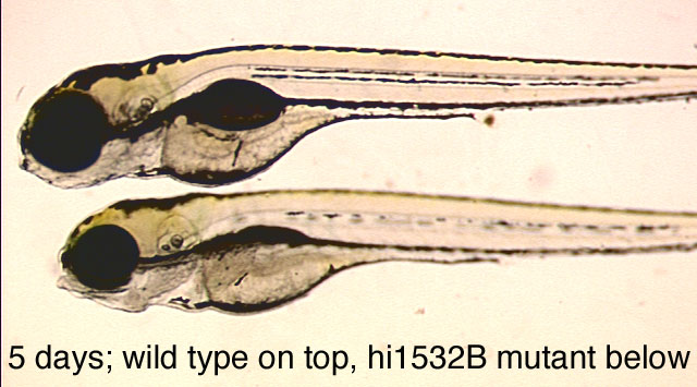
Example of histological images of wild-type (normal) and mutant zebrafish at age 7 dpf. Images taken from Penn State Zebrafish Atlas [28]; direct link to virtual slide comparison tool at http://zfatlas.psu.edu/comparison.php?s[]=264,1,382,172&s[]=265,1,474,386

Compared to gross phenotypic characterization using stereomicroscopy, the microscopic analysis of histological samples is more expensive in terms of time and effort. While recent technological advancements [32, 36] have enabled the largely automatic collection of high-throughput histological data in the form of libraries of high-resolution “virtual slides” of zebrafish larval histology [28], the annotation and scoring of histological data has remained a manual, subjective, and relatively low-throughput process. While useful clinically, the qualitative aspects of current histological assessments can be associated with intra- and inter-observer variability [5] due to variations in observer training, ability, timing, experience, and alertness. Therefore, in order to maximize the effectiveness of histological studies as applied to animal model systems, it is critical that some form of automatic, quantitative method be developed for the analysis of histology images.

We have been actively researching methods in content-based image retrieval (CBIR) and annotation with the goal of developing a fully automated system that is not only capable of scoring defects in zebrafish histology, but is also compatible with the high-throughput histology workflow that we have previously proposed [32] (see Fig. 3). In 2007, we developed the first system [2] for automated segmentation, feature extraction, and classification of zebrafish histological abnormalities, with a pilot study focusing specifically on the larval-stage eye and gut organs, which were chosen because of their inherent polarity and “directional” organization that, when disrupted, results in mutant phenotypes that are relatively easy for human experts to detect (see Fig. 4 for examples of normal versus mutant eye histology). Our prototype system proved to be a successful proof-of-concept, demonstrating that even conventional approaches to image segmentation and classification had the potential not only to distinguish normal (or “wild-type”) tissue from abnormal, but also to classify the abnormality according to different levels of severity, yielding a “semi-quantitative” result.

Fig. 3

An overview of the high-throughput histology workflow (modified from Sabaliauskas et al. [32])

Fig. 4

Example of histological images of wild-type (normal) and mutant zebrafish eyes at age 5 dpf (days post fertilization)

While this prototype system was comparatively slow and not necessarily designed for high-throughput or high-resolution use, it nonetheless provided the foundation upon which we have developed the present work, which we call SHIRAZ (System of Histological Image Retrieval and Annotation for Zoomorphology). Presently, SHIRAZ is designed to process high-resolution images of larval zebrafish arrays directly at 20× magnification (presently corresponding to approximately 0.5 μm per pixel). The current prototype system enables the automatic extraction of individual specimens from the array (comprised of histological sections of up to 50 larval specimens, all on a single slide), followed by extraction of the eyes, which are then automatically annotated according to the presence of histological abnormalities. SHIRAZ has the potential to discriminate between different types of abnormalities, whether they be morphological phenotypes resulting from genetic mutations or tissue artifacts that may have arisen during the high-throughput histology workflow. The work described herein thus makes the following contributions to the biological and multimedia retrieval research communities:

• 1. The first content-based image retrieval system designed to rapidly annotate both histological phenotypes and potentially confounding artifacts;

• 2. A novel similarity scheme for multi-label classification, based on a combination of information-based and probabilistic approaches; and

• 3. A proof-of-principle demonstration of a prototype system enabling greater phenotyping efficiency to benefit large-scale phenotyping projects, such as the Zebrafish Phenome Project described above.

Before describing in detail the technical challenges and our proposed solutions, however, it is prudent to briefly review here the CBIR field and its relevance to the biological community.

2 Related work

Conventional image retrieval methods in use today, such as Yahoo! Image Search [40], are often described as description- or text-based image retrieval systems [24]. In such systems, images in a database must be annotated manually with a series of keywords (“metadata”) so that the images may be found in a text-based search query. However, manual annotation is time-consuming and may ignore key features depending on the annotator’s expertise and diligence. Context-based indexing methods attempt to automatically assign keywords to images on the Web based on the proximity of keywords or other textual metadata to an image filename in the context of the document in which the image and text appear, but the success of such an approach is limited by, in part, the accuracy (and disambiguity) of the textual metadata themselves, which in many cases were entered manually anyway, potentially introducing the same difficulties for retrieval precision as direct manual annotation in a database. On the other hand, in CBIR systems, images are searched and retrieved (and in some cases, automatically annotated) according to their visual content [24] rather than on manually entered keywords or metadata. In general, there are three main parts to any CBIR system: feature extraction, indexing, and retrieval. When an image is processed, the visual features of an image—such as texture, color, and shape—must first be extracted. These low-level features are represented by a multidimensional index or “feature vector” and then stored in a database. Relevant images in the database are returned as matches to a query based on some measure of “distance” between the feature vectors of the query and database images.

The idea of using image or video content to query a database is nothing new. The QBIC (Query By Image Content) method, introduced in 1993 by IBM [26], inspired a number of related CBIR systems, including the SIMPLIcity system [38], which made novel use of semantically-adaptive searching methods. When a query image is submitted to SIMPLIcity, the image is segmented into similar regions and then classified as either a photograph or an illustration, for example. This semantic classification thus dictates the choice of algorithm to be used for feature extraction.

In a related project, the Automatic Linguistic Indexing of Pictures (ALIP) system [19] is used to train computers to automatically recognize and annotate images by extracting their features and comparing them to categories of images that have previously been annotated. The demonstrated high accuracy of the ALIP system’s potential to index photographic images compelled the development of a computationally much more efficient statistical modeling algorithm and a Web-based user interface, ALIPR, to permit users to upload images and see the results of the annotation in real time [20]. For details on these and other technical approaches and progress made in the CBIR field, the surveys by Smeulders et al. [34] (covering the pre-year 2000 period) and Datta et al. [7] (2000–2008) together provide a comprehensive review.

Computational symmetry for novel image retrieval and machine vision applications

A largely unexplored approach to image characterization and retrieval is based on the recognition of symmetry patterns in certain images. Patterns that exhibit 1-D symmetry and repetition are known as “frieze” patterns, and their 2-D counterparts are known as “wallpaper” patterns. Studies involving the application of group theory to pattern recognition show that there are only seven unique frieze symmetry groups and only 17 unique wallpaper groups, enabling the possibility of systematic methods for pattern characterization, even in noisy or distorted images [13]. Each frieze pattern corresponds to particular rotational symmetry group, whether cyclic or dihedral, as demonstrated by Lee et al. [18], who recently proposed a new algorithm for rotational symmetry detection using a “frieze-expansion” approach, in which 2-D images consisting of potential centers of rotational symmetry are transformed from polar to rectangular coordinates with respect to each potential symmetry center. The local regions of rotational symmetry are then characterized based on the frieze groups detected in the rectangular patterns that result from frieze-expansion. Most real-world images, however, do not immediately exhibit the type of regularity that is easily characterized by frieze or wallpaper symmetry groups. Consequently, near-regular texture (NRT) has been defined [22] as minor geometric, photometric, and topological deformations from an otherwise translationally symmetric 2D wallpaper pattern. Much progress has been made in the automated detection of NRT patterns, whether static [17, 22] or in motion [21]. In addition, the application of computational symmetry methods to the detection and characterization of patterns in histology images was explored in some of our earlier work, with results promising enough to warrant further investigation and more advanced algorithm development, including [3, 4], and the current work.

Recent efforts in automated histological image analysis and retrieval

As noted above, histopathological assessments may suffer from intra- and inter-observer variability [5, 31], which has inspired the development of automated cancer diagnosis systems that make use of advances in machine vision. Several reviews cover the literature related to CBIR systems as applied to biomedical applications, including a general survey by Müller et al. [25] as well as a more recent perspective by Zhou et al. [44] on the role of semantics in medical CBIR systems. In addition, Demir and Yener [9] offer a specialized review of cancer diagnosis systems using automated histopathology.

In one early example of such a system, Hamilton et al. [15] used texture feature extraction and a linear classifier to identify possible locations of dysplastic mucosa in colorectal histology images. In another study, Zhao et al. [43] noted that classification performance might be improved by using a “hierarchy” of classifiers. For instance, one scheme might be used to classify a feature as gland or not-gland, and then depending on the result, a different method would be used to further analyze the image and extract the appropriate features. This paradigm is not unlike the semantically-adaptive searching methods used in the SIMPLIcity method mentioned above [38].

The idea of retrieving histological images based on semantic content analysis was also explored by Tang et al. [35] who used a hierarchy of “coarse” and “fine” analyzers for detection of visual features and semantic labeling of the histological structures and substructures, demonstrating the concept of associating “high-level” semantic content and reasoning with “low-level” visual features and properties, thus laying the groundwork for the development of histological image retrieval systems that not only recognize features of such images, but can also produce meaningful annotations. The concept of a hierarchical, “coarse-to-fine” multiresolution analysis was also investigated by Doyle et al. [10] and by Gurcan et al. [14], who noted that such a framework more closely emulates the histology image process used by human pathologists, and that execution times using this approach can be reduced by an order of magnitude versus single-resolution image retrieval systems.

CBIR systems for the biological community

Beyond the more clinically-oriented CBIR systems mentioned above, the scientific community has begun to embrace CBIR as means for the navigation and high-throughput population of biological databases. A prime example of this effort comes from the laboratory of Eric Xing, who developed a system [12] for querying databases of Drosophila melanogaster (fruit fly) embryo gene expression images using multiple modes, allowing users to query not only by gene name or keyword (as with most biological databases) but also by directly uploading images of gene expression. The system automatically annotates the uploaded image using a list of ranked gene expression terms and returns both a set of similar images as well as a list of relevant genes that produce similar expression patterns. This vastly reduces the complexity of user queries required to find genes that match a given expression pattern (which often involves inputting a complicated series of filtering conditions), making this is an important contribution to bioinformatics. The fact that a gene is expressed in a given tissue, however, does not necessarily mean that the morphology of the tissue will be affected if the underlying gene expression is disrupted. This motivates the need to develop CBIR systems that can be used to annotate images with histological phenotypes. The present work, SHIRAZ, is intended to be the first such system that can do so at high-resolution and with the potential for high-throughput. This scalability would serve the needs of large-scale phenotyping efforts such as the Zebrafish Phenome Project.

3 Methods

3.1 Slide preparation and image preprocessing

Wild-type (i.e., free of genetic manipulation) and mutant zebrafish larvae, at ages ranging from 2 to 5 dpf (dpf = days post-fertilization) were collected, fixed, and embedded as described in [32, 36]. Individual slides containing up to 50 hematoxylin and eosin (H&E)-stained larval zebrafish sections were digitally captured at 20× magnification using an Aperio ScanScope™ slide scanner in the Penn State Zebrafish Functional Genomics Core Imaging Facility. The resulting images are stored in the proprietary SVS (ScanScope Virtual Slide) format. The SVS format is similar to BigTiff or Zoomify formats in that the image files consist of several image layers, with each layer corresponding to a specific resolution or magnification. Generally speaking, the 20× layer alone has a size of approximately 90,000 × 45,000 pixels, roughly corresponding to a ∼150–200 MB uncompressed TIFF file, although many virtual slides in our laboratory have also been digitized at 40× magnification, resulting in even larger (up to ∼50 GB) file sizes (Cheng lab, unpublished).

For our proof-of-principle prototype system, we elected to train SHIRAZ to perform automatic phenotypic annotation of 5 dpf specimens of larval eye histology. For training and testing purposes, a total of 176 pre-selected eye images were manually extracted at full 20× magnification (yielding 768 × 768 single-layer RGB images in TIFF format) using Aperio ImageScope™ software. To enable compatibility with the Web-based SHIRAZ demo site, these images were then converted from TIFF to 24-bit PNG (Portable Network Graphics) format using the ImageMagick mogrify utility.

3.2 Preparation of eye images for texture feature extraction

3.2.1 Extraction of individual histological specimen images

The original 20X SVS file must be split into separate TIFF images. Here, this is accomplished using the tiffsplit command line utility, which itself is part of the libtiff library included with most Linux distributions. Splitting the SVS file up into separate images allows us to perform automated extraction of individual specimens at the lowest possible resolution, with much faster results than would be achieved by processing the original 20X image directly.

The specimens are extracted at low resolution using a fully automated, fiduciary marker-free lattice detection algorithm that we developed previously [3] (see Fig. 5 for a typical “before-and-after” result example). The coordinates of the lattice are scaled up to 20X to enable extraction of individual specimen images at their original resolution. The lattice detection algorithm proceeds in three stages; in stage 1 (Fig. 6a and b), the rotation offset of the array image, if any, is corrected so that all specimens are oriented horizontally. In stage 2 (Fig. 6c and d), we use the detected number of cells in the array to divide the bounding box circumscribing the specimens into an initial lattice, taking advantage of the upper bounds of five columns and ten rows imposed by the histology array apparatus design. In practice, we have observed that is it sufficient to assume that the lattice will contain ten rows, even if some rows are partially or totally unoccupied. The number of columns in the field of view, however, varied from 1 to 5, depending on the particular experimental question. Finally, in stage 3 (Fig. 6e), we optimize the initial lattice by varying its height until we maximize the symmetry of each lattice cell image about its horizontal reflection axis. The algorithm pseudocode is provided as follows:

Stage 1: Global orientation correction

• 1 $A_{\rm convhull}\gets$ area of convex hull

• 2 $A_{\rm box}\gets$ area of bounding box around convex hull

• 3 $\Theta_{\rm corrected}\gets {{\rm argmax}({A_{\rm convhull} \over A_{\rm box}})}$

Stage 2: Rigid lattice placement

• 4 Perform morphological closing (⊕) in vertical direction

• 5 $n_{\rm columns}\gets$ number of connected components after ⊕

• 6 $n_{\rm rows}\gets$ 10 (assumed)

• 7 $L_{\rm initial}\gets$ result of dividing bounding box around foreground pixels into lattice containing (n_rowsn_columns) equally sized cells

Stage 3: Deformable lattice optimization

• 8 foreach grayscale cell image C in lattice L

• 9      $S_{\rm corr}\gets corr\bigl(C, mirrorimage(C)\bigr)$

• 10      $L_{\rm f\/inal}\gets {\rm argmax}(S)$ for all C

Fig. 5

Typical example of a histological section of a larval zebrafish array (left) and its computationally detected underlying lattice structure (right)

Fig. 6

Illustration of the array image lattice detection procedure

The final lattice (L _final) is scaled up from the low resolution image to the full 20X image to enable the full-resolution extraction of specimens; however, any rotation correction applied to the low-resolution image must also be applied to the 20X image as well before the lattice can be applied. We used the VIPS image processing libraries [37] for handling the requisite rotation transformations (using package im_affinei_all) and extractions of those image areas corresponding to individual specimens (using package im_extract_area).

3.2.2 Eye extraction

After the whole-larva specimens are cropped from the source array image, the organs of interest (here, the left and right eyes) are automatically extracted from each specimen image. Relative to the major axis and mouth of the zebrafish larva, the positions of the eyes are highly consistent from one fish to the next. Figure 7 indicates the distribution of overlapping areas of zebrafish left and right eyes (at age 5 dpf) for approximately 45 manually-labeled histological specimens. Because the positions of the eyes are highly consistent for informative specimens, we can use the position of the overlapping areas to crop a 768 × 768 region from each 20X larval specimen image in which the eye histology is contained (assuming that the eye tissue is present in the histological section of interest).

Fig. 7

When each 5-dpf larval zebrafish image is rotated to align to a common origin point (here, the mouth, located at the leftmost position on the midline in the above images) and also along a common horizontal axis, we find that the positions of the eyes across all images are largely overlapping, which allows us to use a relatively simple location-based method for extracting a 768 × 768 square region around each eye for input to the SHIRAZ system

3.2.3 “Frieze-like” expansion of eye histology images

Upon inspection of any typical zebrafish histology image, one can observe that certain tissue structures exhibit a certain degree of repetition or symmetry (at least in the normal or wild-type state). One can see that the zebrafish larval retina possesses partial rotational symmetry about the lens, as indicated in Fig. 8. The repeating pattern implied within the retina might become more obvious (and more easily detected computationally) if the image could be transformed from its rotationally symmetric appearance to a more regular, linear shape, thereby reducing the pattern complexity to only one dimension. This would facilitate the generation of methods for detecting and characterizing the implicit symmetry patterns as well as defects and local deviations that disrupt the pattern continuity. We refer to the transformation of the original eye image into a rectangular shape as frieze-like expansion after the previously mentioned algorithm (see Section 2) by Lee et al. [18] that was designed to locate and characterize the underlying frieze (1-D) symmetry group patterns within real-world images exhibiting local rotational symmetries.

Fig. 8

Labeled layers of the 5-dpf zebrafish eye. In addition, the arrow indicates the direction of the implicit “rotational symmetry” in certain histology images such as this, where we typically find a constant and repeating pattern of cellular layers that revolve about the lens

The zebrafish eye consists of several distinct layers, including the lens, the ganglion cell layer, the inner plexiform later, the inner nuclear layer (which itself consists of the amacrine and bipolar cell layers), the outer plexiform layer, the photoreceptor layer, and finally the retinal pigmented epithelium (RPE) and choroidal melanocytes (which at this developmental stage appear together and have no clear boundary between them) [27] (see Fig. 8). For the purposes of expanding the retina into a 1-D frieze-like pattern, we only need to provide an outer perimeter, which will correspond the top edge of the frieze-like expansion pattern, and an inner perimeter, corresponding to the bottom edge (see Fig. 9). Thus we need only extract the RPE and the lens, and fortunately, they are relatively easy to identify. The RPE, by virtue of its melanin pigmentation, is generally the darkest continuous segment of the retina, and the lens is generally the largest object near the center of the eye image whose shape most closely approximates that of a circle. The image processing operations required for segmentation of the lens and RPE are thus relatively straightforward, consisting primarily of gray-level thresholding, edge detection, and shape identification based on the ratio of the shape’s area to its perimeter (i.e., one possible measure of shape “compactness”).

Fig. 9

Overview of frieze-like expansion of zebrafish retina. Note that because of the distortion resulting from re-scaling the shorter line segments (generally found near the marginal zones of the retina, on either side of the lens), we extract only the middle 50% of pixels (dashed line) from the frieze-expanded eye image

The perimeter points are used as a basis for extracting line segments of pixels from the original eye histology image (Fig. 9a and b). Ideally, each line segment would start at the outer perimeter and be oriented more or less perpendicular to the tangent line at the starting point. The intersecting point on the inner perimeter would thus be the endpoint of the line segment. However, owing to the irregular shape of both perimeters, the line segment may not necessarily end at the desired point on the inner perimeter; in fact, in some cases the line perpendicular to the tangent line at the starting point may not even intersect with the inner perimeter at all. To remedy this, the algorithm identifies a set of initial “control points” evenly spaced around the outer perimeter (in practice, 12 control points usually provides good results). Line segments are extracted starting from these control points and ending at the nearest point on the inner perimeter as measured by Euclidean distance. The remaining line segments are then extracted by interpolation between the control points. Following extraction of all line segments, we normalize their lengths to a pre-specified number of pixels. The normalized line segments are then rearranged as columns of the transformed image (Fig. 9c). Since the layers of the larval retina exhibit only partial rotational symmetry around the lens, the resulting image will be distorted at either end of the frieze expansion. Generally speaking, the central part of the transformed image is most highly representative of the retina’s partial rotational symmetry around the lens, so we perform our subsequent analysis only on this central region (we chose the middle 50% of pixels), and ignore the more highly distorted sections at either end of the original transformed image.

3.3 Extraction of texture features from image blocks

3.3.1 Blockwise processing

Our feature extraction process follows a block-based scheme, in which we divide the frieze-expanded eye image into a series of 64 × 64 blocks (see Fig. 10). Although the height of each frieze-expanded image is set at a fixed 128 pixels, the width of the image will vary from image to image depending on the number of line segments extracted during the frieze-like expansion process. In practice, the width typically ranges from about 400–700 pixels.

Fig. 10

Illustration of subdivision of frieze-expanded eye “parent” image into 64 × 64 “child” block images (Selected image blocks from the subdivision of the parent image have been marked with dotted borders to show their corresponding positions in the “exploded” view)

Dividing the “parent” frieze-expanded image into smaller “child” blocks offers several benefits over extracting features from the parent image as a whole. First, because the local image texture properties will vary throughout the image, extracting features from smaller blocks permits us to more precisely identify where the local texture aberrations occur. If we were to extract features from the image as a whole, it is likely that local variations would be “masked” by the properties of the whole image, thus making it difficult to discriminate or differentially classify two images that are largely identical save for local texture variations.

The blockwise operation also allows us to identify local features in a regional context. The blocks are not necessarily image patches with discrete boundaries—rather, we intend for these blocks to overlap, so that we can approximately capture the “continuum” of local texture variation from one image region to the next, which is particularly important when there are local texture irregularities in the parent image (see Fig. 11). In the vertical direction, where the parent image is 128 pixels high, we extract three 64 × 64 blocks. The top and bottom blocks do have a discrete boundary, but the middle block now overlaps one-half of each of the top and bottom blocks. Because the texture features extracted from the middle block will capture the local variation about the interface between the top and bottom blocks, the three-dimensional “vector” of features representing the three 64 × 64 blocks will be more representative of continuous local variation in the vertical direction than one would obtain by only extracting features from non-overlapping blocks. Conceptually, the idea is similar to taking a “moving average” of variation along the vertical direction, but here we are using a 64 × 64 “window” in which the “moving average” is computed.

Fig. 11

An example to illustrate the rationale for using overlapping child block images

In the horizontal direction, a similar approach is taken, but because the width varies from one image to the next, the number and location of the individual 64 × 64 blocks or “windows” will also vary. In other words, the image width is usually not a multiple of 64, and so dividing up the image into non-overlapping patches will result in a “remainder” set of pixels that is less than 64 pixels wide. Allowing for overlap as was done in the vertical direction, where the overlapping blocks cover one-half of each of their neighbors, would only work if the parent image width were a multiple of 32. To ensure account for all pixels in the parent image, we still allow for overlap from one block to the next, but the extent of overlap—in terms of the number of pixels along the horizontal—is now a function of the total width of the parent image. To compute both the degree of overlap and the number of “child” blocks to be extracted in the horizontal direction while ensuring that the extent of pixel overlap is identical for all blocks and that no pixels are left unaccounted for, we devised the following procedure:

$$ \begin{array}{l} \textit{width} \gets \mbox{ width of frieze-expanded parent image} \\ \\ \textit{height} \gets \mbox{ height of frieze-expanded parent image}\\ \\ \textit{blocksize} = {\it f\/loor}\left(\frac{\textit{height}}{2}\right)\\ \\ \beta = {ceil\left({\frac{\textit{width}} {\textit{blocksize}}}\right)} \\ \\ \alpha = \textit{blocksize} - {\frac{(\textit{blocksize} \times \beta) - \textit{width}} {\beta - 1} } \end{array} $$

In the above algorithm, β represents the number of blocks to be extracted, while α represents the degree of horizontal overlap between blocks, expressed in number of pixels. (The degree of overlap in the vertical direction is always 32, assuming that the parent image height is always 128.) For each 64 × 64 image block, we extract a total of 54 features, comprised of a combination of the following:

• Gray-level co-occurrence features

• Lacunarity

• Gray-level morphology features

• Markov Random Field model parameters

• Daubechies wavelet packet features

We describe each of the above five types of features in more detail below.

3.3.2 Gray-level co-occurrence features

A common method for characterizing texture in images involves descriptors derived from an image’s gray level co-occurrence matrix, or GLCM, which is a representation of the second-order (joint) probability of pairs of pixels having certain gray level values. For a given pixel (i, j) which has a gray-level value m, the GLCM provides a method of representing the frequency of pixels at some distance d from (i, j) that have a gray-level value n. Formally, a rotationally-invariant GLCM (that is, one that only depends on the distance (Δx, Δy) between pixels in a pair, and not on the angle of the line segment connecting them) may be defined as

$$ C(m,n,{\Delta}x,{\Delta}y) = \sum\limits_i \sum\limits_j I\bigl(m-g(i,j)\bigr)I\bigl(n-g(i+{\Delta}x,j+{\Delta}y)\bigr) $$

(1)

where C is the GLCM, g(i, j) represents the gray level value at position (i, j), Δx and Δy are respectively the offset distances in the x and y directions, and the binary indicator function I(a − b) equals 1 if a = b, but equals zero if a ≠ b.

The GLCM is a rich representation of the texture contained in an image, but by itself it is large and often sparse, and thus cumbersome to work with. In practice, one can compute a series of second-order statistics from the GLCM that provide a more compact representation of image texture. The five most common descriptors computed from the GLCM and which we use in our analysis are listed below, shown here as defined in [29] but originally derived by Haralick et al. in [16]:

• Energy:

  $$ \displaystyle\sum\limits_{m=0}^{L-1}\sum\limits_{n=0}^{L-1}p(m,n)^2 $$

  (2)

• Entropy:

  $$ \displaystyle\sum\limits_{m=0}^{L-1}\sum\limits_{n=0}^{L-1}p(m,n) \log p(m,n) $$

  (3)

• Contrast:

  $$ {1\over{(L-1)^2}}\displaystyle\sum\limits_{m=0}^{L-1}\sum\limits_{n=0}^{L-1} (m-n)^2 p(m,n) $$

  (4)

• Correlation:

  $$ {\sum\nolimits_{m=0}^{L-1}\sum\nolimits_{n=0}^{L-1}mnp(m,n)-{\mu}_x{\mu}_y}\over{\sigma_x\sigma_y} $$

  (5)

  where

  $$ \mu_x = \displaystyle\sum\limits_{m=0}^{L-1}m\sum\limits_{n=0}^{L-1}p(m,n) \quad\quad\quad\quad\quad \mu_y = \displaystyle\sum\limits_{n=0}^{L-1}n\sum\limits_{m=0}^{L-1}p(m,n) $$
  $$ \sigma_x = \displaystyle\sum\limits_{m=0}^{L-1}(m - \mu_x)^2\sum\limits_{n=0}^{L-1}p(m,n) \quad\quad \sigma_y = \displaystyle\sum\limits_{n=0}^{L-1}(n - \mu_y)^2\sum\limits_{m=0}^{L-1}p(m,n) $$

• Homogeneity:

  $$ \displaystyle\sum\limits_{m=0}^{L-1}\sum\limits_{n=0}^{L-1} {{p(m,n)}\over{1 + |m-n|}} $$

  (6)

In each of the above formulae, L refers to the total number of gray levels (256 for an 8-bit image), and p(m, n) is the joint probability density function derived by normalizing the co-occurrence matrix C via division by the number of all paired pixel occurrences, i.e.:

$$ p(m,n) = {{C(m,n)}\over{\rm total\ number\ of\ paired\ occurrences}} $$

(7)

3.3.3 Lacunarity

To enhance the description of an image’s texture beyond the Haralick texture features described above, we also employ a measure known as lacunarity, which is perhaps more commonly used in geometry as a measure of fractal texture [30], but we use it here as a means of representing the heterogeneity of image data. Mathematically, it is similar to the so-called “dispersion index” in that it depends on the ratio of the variance of a function divided by its mean. Lacunarity can be described by any of the following expressions (as defined in [29]):

$${\mathcal{L}_s \equiv {{1\over NM} \sum\nolimits_{i=1}^N \sum\nolimits_{j=1}^M g(i,j)^2 \over {\left({1\over NM} \sum\nolimits_{k=1}^N \sum\nolimits_{l=1}^M g(k,l)\right)^2}} - 1} $$

(8)

$${\mathcal{L}_a \equiv {1\over NM} \displaystyle\sum\limits_{i=1}^N \displaystyle\sum\limits_{j=1}^M {\Bigg|{ g(i,j) \over {\left({1\over NM} \sum\nolimits_{k=1}^N \sum\nolimits_{l=1}^M g(k,l)\right)}} - 1}\Bigg|} $$

(9)

$${\mathcal{L}_p \equiv {\Bigg({1\over NM} \displaystyle\sum\limits_{i=1}^N \displaystyle\sum\limits_{j=1}^M {\Bigg({ g(i,j) \over {\left({1\over NM} \sum\nolimits_{k=1}^N \sum\nolimits_{l=1}^M g(k,l)\right)}} - 1}\Bigg)^p}\Bigg)}^{1\over p} $$

(10)

Respectively, $\mathcal{L}_s$, $\mathcal{L}_a$, and $\mathcal{L}_p$ refer to the squared, absolute, and power-mean representations of lacunarity, while g(i, j) refers to the gray-level value of the pixel located at (i, j). In our analysis, we extract lacunarity features for $\mathcal{L}_s$, $\mathcal{L}_a$, as well as $\mathcal{L}_p$ at three arbitrarily chosen levels: p = 2, p = 4, and p = 6.

3.3.4 Gray-level morphology

In image processing, morphological operations such as dilation, erosion, opening, and closing are often used to generate representations of the shapes of image regions, which may then be used in the segmentation of images into regions of similar color and/or texture. Typically, morphological operations are performed on black-and-white or “binarized” images—that is, images that have been thresholded at a particular gray level value such that image pixels at or above the threshold value are re-mapped as “foreground” pixels (with a value of 1), and all other pixels are re-mapped as “background” pixels (with a value of 0). Morphological operations are applied to each pixel in the image in order to add or remove pixels inscribed within in a “moving neighborhood” (known as a structuring element) centered on each pixel in the source image. In dilation, for example, the source image is modified by placing the structuring element over each foreground pixel and then setting all pixels within the contained area to a value of 1. The effect is that all objects in the foreground are expanded or “dilated,” as the name suggests. By contrast, in erosion, the foreground objects are modified by placing the structuring element over each object pixel and then removing or “eroding” object pixels that do not allow the structuring element to fit within the object. For example, if we place a 3 × 3 square structuring element over a given foreground object pixel, the resulting output image will only keep that object pixel if all of its eight-connected neighbors are foreground pixels. If even one of its eight-connected neighbors are background pixels (i.e., having a value of zero), then the central object pixel is removed, or “eroded,” and will not appear in the resulting output image.

Dilation and erosion are typically used in combination when the goal is to remove object details that are smaller than a given size while leaving larger details alone [29]. For example, to remove spurious, “hair-like” projections from an object, we would first erode the image to remove the spurious details, and then perform dilation on the eroded image to restore the more “solid” portions of the image objects to their original sizes. The process of erosion followed by dilation is more commonly known as opening. In contrast, we may choose to perform closing on an image if there are spurious or otherwise undesired “gaps” within an image object. To “close” an image, we first perform dilation on the foreground pixels to “cover up” the gaps, and then we perform erosion on the result to restore the gap-filled objects back to their original sizes. The success or failure of opening and closing in accomplishing the user’s objective depends, of course, on the type and size of structuring element used. If there are wide gaps within an object, the user would want to employ a structuring element whose radius was wide enough to ensure gap closure, but not so wide as to merge two or more distant objects that are unrelated (i.e., not intended to be part of the same closed region).

Morphological operations may also be applied to the gray-level images themselves, without the need for thresholding or “binarization,” with the main difference being that when placing the structuring element over the central pixel, only the central pixel will be modified. In the output image, the central pixel takes on the value of the maximum (if dilation) or minimum (if erosion) gray level of the pixels within the neighborhood covered by the structuring element, while the remaining pixels under the structuring element are ignored. This difference in the operation ensures that the same output image is obtained regardless of how the structuring element “moves” around the source image. In other words, if all pixels under the structuring element were set to the value of the maximum- (or minimum-) gray value pixel, then every time the structuring element moved to a new position, the output values of non-central pixels covered by the structuring element in the previous position may change. A structuring element that moves, for instance, from left-to-right will produce a different output image than one that moves from right-to-left. By allowing only the central pixel to be modified, the same output image will be produced regardless of the path followed by the structuring element.

The results of applying morphological operations on a gray-level image may be useful in characterizing the texture of the image by granulometry, using the following method as described in [29]:

• S _D = result of dilating gray level source image S using a structuring element of radius m

• S _E = result of eroding gray level source image S using a structuring element of radius m

• N₁ = sum of the pixel values of the difference image produced by subtracting S _E from S _D

• N₂ = sum of the pixel values of the original image S, excluding the values at pixels that were “ignored” by the dilation and erosion operations (i.e., the pixels around the image perimeter)

• N₁/N₂ = granulometry of image S

3.3.5 Markov random fields

Markov random fields (MRFs) have been used to model image textures; some of the earliest work in the area comes from Cross and Jain [6]. A random field, in its most general sense, may be represented by a series of random values (such as the outcomes of a coin tossing or other random number generation experiment) mapped onto some n-dimensional space. In the case of two-dimensional images, n = 2, and the random field might consist of a set of randomly selected gray levels placed on the two-dimensional grid.

A Markov random field is similar, but instead of each pixel’s gray level value being determined by an unbiased random experiment, the gray-level value of each pixel possesses a so-called “Markovian” property in that the gray level value is directly dependent on or influenced by the pixels in its immediate neighborhood (but not directly dependent on pixels outside of that neighborhood). By implicit determination of Markov random field parameters, we may be able to model the gray levels that constitute a particular image’s texture.

In our analysis, we use the parameters of a Gaussian MRF model as texture features. A Gaussian MRF has the following properties:

• The value of each pixel is determined by a random sample from a Gaussian distribution

• For a given pixel value, the parameters of the Gaussian distribution are functions of the values of the neighboring pixels

For simplicity, the standard deviation of the Gaussian may be assumed to be independent of the gray values of the neighbors about the central pixel (but which is still characteristic of the Markov process), and so a general model for the Gaussian MRF can be represented by the following probability density function:

$$ p\bigl(g_{ij}|g_{i'j'},(i',j') \in N_{ij}\bigr) = {1 \over {\sqrt{2\pi}\sigma}}\exp\left({{{-{\bigl(g_{ij}-\sum\nolimits_{l=1}^{L}a_l g_{i'j';l}\bigr)^2}}}\over{2{\sigma}^2}}\right) $$

(11)

in which $p\bigl(g_{ij}|g_{i'j'},(i',j') \in N_{ij}\bigr)$ represents the probability of pixel (i, j) having gray-level value g _ij given the corresponding gray-level values of the neighboring pixels, L is the number of pixels in the neighborhood defined by N _ij that influence the pixel (i, j) in the context of the MRF, a _l is a MRF parameter indicating the level of influence that a neighbor pixel has on the pixel at (i, j), and g _i′j′;l is the value of the neighbor pixel at the position (i′, j′). Finally, the standard deviation σ is an expression of the degree of uncertainty in the Gaussian MRF model and is also used to characterize the random experiment performed in each location that the model uses to assign a value to pixel (i, j) [29].

One method of inferring the parameters of a Gaussian MRF is by least-squared-error (LSE) estimation. We follow the LSE estimation procedure outlined in [29]. If, for example, we assume a second-order Markov neighborhood in which the neighboring pixels are immediately adjacent to the central pixel (i.e., an eight-connected neighborhood), then the above equation becomes

$$ p\bigl(g_{ij}|g_{i'j'},(i',j') \in N_{ij}\bigr) = {1 \over {\sqrt{2\pi}\sigma}}exp\left({{{-{\bigl(g_{ij}-\sum\nolimits_{l=1}^{4}a_l s_{ij;l}\bigr)^2}}}\over{2{\sigma}^2}}\right) $$

(12)

where:

$$\begin{array}{lll} && s_{ij;1} \equiv g_{i-1,j} + g_{i+1,j} \nonumber \\ && s_{ij;2} \equiv g_{i,j-1} + g_{i,j+1} \nonumber \\ && s_{ij;3} \equiv g_{i-1,j-1} + g_{i+1,j+1} \nonumber \\ && s_{ij;4} \equiv g_{i-1,j+1} + g_{i+1,j-1} \end{array}$$

(13)

and thus five parameters must be determined implicitly: a ₁, a ₂, a ₃, a ₄, and σ. These five parameters can thus be used as properties of the image texture modeled by the Gaussian MRF. However, a proper solution of the model can only take place simultaneously for those pixels that have non-overlapping neighborhoods of pixels that influence the central value according to the model. In the case of the second-order (eight-connected) neighborhood used here, it can be shown that an image can be divided up into four possible sets of pixels whose influencing neighbors do not overlap [29]. Thus, we can compute the five parameters a ₁, a ₂, a ₃, a ₄, and σ for each of these four sets of pixels, and also take their respective means, and then use all of these results as texture features. For the LSE-MRF texture modeling approach alone, this yields a fairly robust 25-feature set for each 64 × 64 image block.

3.3.6 Wavelet packet features for texture characterization

More recently, wavelets have become a popular form of multiresolution representation of image texture. In the context of signal and image processing, wavelets are used to break down a function or signal into components at multiple scales, yielding insight not only into an image’s frequency characteristics, but its spatial characteristics as well [11].

In practice, the multiresolution analysis is performed by applying low- and high-pass filters along the vertical and horizontal axes of a full-resolution image (a low-pass filter passes lower-frequency signals and reduces higher-frequency signal amplitudes, while a high-pass filter does the opposite). This results in a “splitting” or “expansion” of the original signal into four component subbands: Low-Low (LL), Low-High (LH), High-Low (HL), and High-High (HH). The LH, HL, and HH subbands provide information about texture variation in the vertical, horizontal, and diagonal directions, respectively [38]. Each of the four subbands can then be filtered again at additional levels of resolution; the expansions from one scale to the next can be visualized as a tree-like structure (see Fig. 12). For the purposes of texture analysis, we wish to have as much redundant information as is computationally feasible to provide a robust representation of image texture, and so it makes sense to expand all signals into their LL, LH, HL, and HH subband components. This “full” expansion is typically referred to as packet wavelet analysis, which stands in contrast to tree wavelet analysis, which focuses only on the lowest frequency subbands and thus is useful for compressing an image into a form where it can be reconstructed from the minimum number of bits [29]. Because we are interested here in the characterization of image texture and not on the compression of image file size, we use the packet wavelet approach in our analysis. Further, rather than always choosing the lowest-frequency channels for signal expansion at each scale, we preferentially choose the subband with the highest “energy,” which is computed by taking the summation of the squares of the gray level values of the pixels making up each subband image. The “energies” at each level are thus used as features for describing the texture of the original image.

Fig. 12

Example of wavelet packet expansion for a 64 × 64 “child” image block taken from a frieze-expanded “parent” image. The expansion proceeds through four steps, and following the initial expansion, the image corresponding to the highest-energy band is chosen for the next level of expansion. A total of 16 energy values are thus used as texture features for each child image block

A number of filters have been developed for wavelet analysis, each having different properties that result in a trade-off between computation time and the ability to capture local texture variation at longer resolutions. The Daubechies-4 filter [8] is a common filter that yields a good combination of localization properties and speed of computation [38], and we thus use it here. In our tests, we found that using the Daubechies-4 filter to expand a 64 × 64 block into four scale levels (preferentially choosing the highest-energy subband at each level) produced acceptable results for generating a large number of texture features (i.e., the “energy” levels of each channel at each level of expansion) in a relatively short period of time.

3.3.7 Summary of feature extraction procedure

To summarize, we extract a total of 54 texture features for each child image block, including five GLCM-derived or “Haralick” features, five lacunarity features, three gray-level morphology features (N ₁, N ₂, and granulometry), twenty-five LSE-estimated MRF properties, and sixteen energy features computed by packet wavelet analysis. In our tests, using feature extraction implementation binaries (compiled for Linux) as provided in [29], a typical frieze-expanded “parent” image yields a full set of texture features (54 features per 64 × 64 child block image, computed for approximately 50–60 blocks depending, for a total of about 3,000 features per parent image) in about 15–20 s. Figure 13 shows an example of the values of features extracted from two images representative of obviously different textures.

Fig. 13

Examples of actual values of texture features extracted from two different image blocks taken from the same frieze-expanded parent image

Once the 54 features are extracted across all 3 × 3 neighborhoods centered on each of the “central blocks,” we re-shape the resulting feature matrix into a set of nine-element vectors, with each vector corresponding to the same texture descriptor extracted across the nine blocks making up each 3 × 3 neighborhood (see Fig. 14). The values in each nine-element vector are sorted in ascending order, somewhat resembling a “cumulative distribution” or other sigmoidal curve, though such a description is given for illustration purposes only. The reason for the sorting of the 9-element vectors is to facilitate the calculation of the degree of betweenness of a “query vector” with respect to two “boundary vectors” that are determined in the training phase, described below in Section 3.4.2.

Fig. 14

Illustration describing how the feature matrix extracted from each frieze-expanded image is reshaped into a series of sorted nine-element feature vectors, one for each feature-neighborhood correspondence

3.4 Feature subset selection and classifier training

3.4.1 Overview of phenotype and artifact annotation concepts

One of the goals of the SHIRAZ system is that it will be able to automatically annotate the phenotype observed in a larval zebrafish histology image based on its similarity to classes of images that have previously been characterized. In practice, however, most larval histology images will contain some sort of artifact that arises during the slide preparation or digitization processes. Typical artifacts may include separation or tearing of cell layers that result from sectioning errors, or the tissue appearance being grossly distorted as a result of poor fixation, or that sectioning may have occurred at a skewed angle (producing a so-called “eccentric” section) because the larval specimen was not properly oriented during the embedding process. A trained observer may be able to account for these artifacts when scoring a histological phenotype, but in certain cases, the artifact may in fact obfuscate the underlying phenotype, and the affected section should not be used. We have, therefore, elected to allow the annotation of larval histology images based not only on a detected phenotype, but also on the detection of artifacts that indicate errors in histological preparation. For the purposes of our demonstration, we have chosen a total of ten possible labels or “concepts” for annotation of images of the larval zebrafish retina:

• 1. Phenotype—absent (i.e., normal or “wild-type”)

• 2. Phenotype—necrosis—minimal to mild

• 3. Phenotype—necrosis—moderate to severe

• 4. Phenotype—disorganization—minimal to mild

• 5. Phenotype—disorganization—moderate to severe

• 6. Phenotype—possible hypotrophy

• 7. Artifact—lens detachment or similar tissue “shrinkage” artifact

• 8. Artifact—lens is abnormal in appearance (dark, small, “chattered,” or undetectable, but can possibly indicate a malformation phenotype)

• 9. Artifact—specimen appears to have fixation problems

• 10. Optic nerve or hyaloid artery appears to be present (neither a phenotype nor an artifact)

Examples of potential phenotype and artifact annotation labels are given in Fig. 15. For feature selection and classification, we wanted to allow for an image to be annotated with multiple labels when appropriate and possible. For example, a retinal image may exhibit a normal phenotype, but the lens may happen to be detached due to a so-called “shrinkage” artifact resulting from improper preparation of the tissue sample.

Fig. 15

Typical example images spanning the range of histological phenotypes and artifacts that SHIRAZ is trained to recognize

For training, we do not assign labels to the parent images as a whole, but rather to the “child” block images—or more specifically, to each of the “central” child blocks and their eight-connected neighbor blocks. For example, let us say that a parent image has been “divided” into three rows of 19 blocks each (for a total of 57 blocks); the “central” child blocks would consist of the set of 17 blocks that are not located along the perimeter (or, put another way, the set of blocks in the middle row, with exception of the two end blocks). Each of the 17 central blocks has eight neighbor blocks, and these neighborhoods will overlap from one central block to the next. Just as we allow the blocks themselves to overlap with each other to provide a more continuous representation of image texture (as in Fig. 11), the overlapping of the 3 × 3 neighborhoods also contributes to a model of such a “texture continuum,” as described above and illustrated in Fig. 14.

An additional benefit to extracting features nine blocks at a time in a 3 × 3 fashion is that we can preserve, to a certain extent, the location-specific context of the image texture information. From a biological point of view, this enables us to discriminate between different degrees of abnormality that may only manifest themselves in local texture aberrations. For example, an image depicting “minimal to mild necrosis” might exhibit a texture anomaly in only one or two blocks in a nine-block neighborhood, while an image of “moderate to severe necrosis” might exhibit similar texture anomalies across a greater number of blocks.

3.4.2 Determination of “feature signatures” for each class

During the training phase, a set of classification “rules” are identified for each annotation concept. We refer to a given concept’s collective set of “rules” as its feature signature, which consists of the subset of 54 features (along with the upper and lower boundaries of the values of such features in the subset) which have been determined to be, statistically speaking, more enriched within that concept than in the other concepts.

For each feature Φ we compute the pairwise information agreement score S between any two image neighborhoods i and j as follows:

$$ S(i,j,\Phi) \equiv \log_2{\mathcal{N} \over {\displaystyle\sum\limits_{k=1}^{\mathcal{N}}}\Bigg[\displaystyle\bigcap\limits_{v=1}^{9}\bigl[\min(s_{{\Phi}iv},s_{{\Phi}jv}) \leq s_{{\Phi}kv} \leq \max(s_{{\Phi}iv},s_{{\Phi}jv})\bigr]_{i{\neq}j}\Bigg]} $$

(14)

where s refers to a single element of the sorted (in ascending order) nine-element vector extracted for a given 3 × 3 neighborhood. The expression min (s _Φiv , s _Φjv ) (or, respectively, max (s _Φiv , s _Φjv )) means that we are taking the lesser (greater) of the two values contributed by the feature vector for the neighborhood pair (i, j) at element position v. Strictly speaking, the use of the intersection notation (∩) would require that all nine elements of the feature vector s _Φkv must lie between the min and max “boundary vectors” defined by neighborhoods i and j, but in practice we allow for up to two of the elements of the feature vector for neighborhood k to fall outside of these limits (similar to the example shown in Fig. 16). $\mathcal{N}$ refers to the total number of neighborhoods in the entire database.

Fig. 16

Illustration of agreement test for a nine-element “query vector” (that is, corresponding to a given 3 × 3 child block neighborhood, as in Fig. 12) and its degree of match to the statistically determined feature signature corresponding to that texture feature (see Sections 3.4.2 and 3.4.3). In practice, we allow for up to two elements to be outside the boundaries before the query vector fails the “betweenness test ” for that texture feature

The above formula is derived from the so-called “loss-of-function agreement score” previously been proposed by Weirauch et al. [39] for characterizing the frequency of phenotypic presence (and/or absence) among a set of genetic mutants. Our variant allows for the possibility of quantitative feature values to be used in the pairwise comparisons of feature vectors, unlike the original metric, which requires that the phenotypic presence be expressed as a logical (that is, the phenotype is simply “present” or “absent”). Mathematically, however, both the above equation and the original metric by Weirauch et al. are based on the concept of the inverse document frequency used in information retrieval [33].

The probability computed from the cumulative hypergeometric distribution function may be used to determine the extent to which a given feature Φ is enriched in the so-called “feature signature” for a class (i.e., the subset of features that tends to belong to a particular class, but not to others). Generally speaking, for each feature Φ, we want to see if the “random sampling” (without replacement) of N elements contains at least x elements that meet some pre-specified criterion for “success.” M refers to the total number of elements in the whole population, while K refers to the number of elements in the whole population that also meet the criterion for “success.” The probability of the event X ≥ x (i.e., that at least x samples drawn meet the “success” criterion) is computed as

$$\label{eq15} P(X \geq x) = 1 - P\bigl(X \leq (x - 1)\bigr) = 1 - \sum\limits_{i=0}^{x-1} {{\dbinom{K}{i}\dbinom{M - K}{N - i}}\over\dbinom{M}{N}} $$

(15)

The resulting P-value tells us the probability that the x successes are due to random chance. If we compute this P-value for every feature Φ and for a given class, then those features with a significant P-value (typically ≤ 0.05, but can be adjusted for stringency) would be considered part of the subset or signature of features that are enriched in that class (and which are less likely to be observed in other classes).

3.4.3 Training procedure

Here we summarize the steps involved in training the SHIRAZ annotation system:

• 1. Divide each frieze-expanded parent image into 64 × 64 child block images, then capture vector of 54 texture features for the 3 × 3 neighborhood about each of the central child blocks.

• 2. Sort each neighborhood’s feature vector as described in Section 3.3.6, then merge all feature vectors into a “feature matrix” $\mathcal{M}$, which will have a total of (54 × 9 = ) 486 features for each row (corresponding to the neighborhood about each of the central child block images). Each neighborhood i of $\mathcal{M}$ is then labeled with a relevant histological phenotype/artifact annotation concept κ.

• 3. Determine the feature signature Ψ _κ associated with a given labeled concept κ, as follows:

  • (a) Compute the pairwise information agreement score (using (14)) for neighborhoods i and j and store as S(i, j, Φ). The total size of S is $\mathcal{N} \times \mathcal{N} \times \mathcal{F}$, where $\mathcal{F}$ is the total number of features = 54.

  • (b) In each symmetric matrix S _Φ (that is, the square $\mathcal{N} \times \mathcal{N}$ matrix corresponding to each feature Φ), each column S _i,Φ corresponds to all pairs of neighborhoods containing neighborhood i, each of which has been assigned a specific annotation concept. Thus, we repeat the following steps for each feature Φ and for each concept κ, while ignoring all pairwise self-comparisons (i, i):

    • i. Determine a minimum agreement score value S _min (e.g., 80th or 90th percentile of all values in S _Φ) required for any two neighborhoods i and j to be considered “similar.”

    • ii. Let x = the number of neighborhood pairs in S _i,Φ that belong to annotation concept κ but for which the criterion S(i, j, Φ) ≥ S _min has been met

    • iii. Let K = the number of neighborhood pairs in S _i,Φ where S(i, j, Φ) ≥ S _min

    • iv. Let N = the number of neighborhood pairs in S _i,Φ that belong to annotation concept κ, regardless of the value of S(i, j, Φ)

    • v. Let M = the total number of neighborhood pairs in S _i,Φ

    • vi. Use x, K, N, and M as inputs to the cumulative hypergeometric distribution function (15) to determine the probability that the number of samples in the class that meet the criteria of interest is due only to random chance (i.e., the P-value). Note that the “random sample” (that is, the set of N elements selected from S _i,Φ above) is not actually random, but corresponds to those samples that have been labeled with the current annotation concept κ whose feature signature Ψ _κ we are trying to determine.

    • vii. If a minimum fraction (we used 80%) of all P-values computed for each class sample are significant (e.g., P ≤ 0.05), then assign the current feature to the feature signature Ψ _κ for the concept κ.

    • viii. Determine the betweenness rules that must be met for a new test sample neighborhood to be assigned with the current concept (see below). In other words, if the current feature Φ belongs to the current annotation concept’s feature signature Ψ _κ , then we let Ψ _κ (Φ)_max and Ψ _κ (Φ)_min equal, respectively, vectors containing the maximum and minimum values with respect to the set of the original nine-element vectors corresponding to the neighborhoods belonging to the current annotation concept κ.

3.4.4 Automated image annotation

A previously uncharacterized eye image I will be annotated as follows:

• 1. Extract the image features for each 3 × 3 child block image neighborhood i in the parent image I. Let X _i,Φ = the nine-element vector (sorted in ascending order) for each feature.

• 2. Initialize Ψ _κ,matches = 0

• 3. For each child image neighborhood in I, for each annotation concept κ, and for each feature/phenotype Φ:

  • (a) If seven out of nine elements in X _i,Φ fall within the betweenness limit vectors Ψ _κ (Φ)_max and Ψ _κ (Φ)_min of the current annotation concept’s feature signature Ψ _κ , then increment Ψ _κ,matches by 1

  • (b) Let n _κ = the total number of features in the feature signature for concept κ

  • (c) Let Φ _κ = the normalized fraction of matches computed over all features in the feature signature Ψ _κ for the current neighborhood = $\Psi_{\kappa,{\rm matches}} \over n_\kappa^2$ (Note: the denominator term is squared in order to account for the variability in the number of features included in each concept’s feature signature and to mitigate the effect of any annotation bias towards concepts that have signatures with a greater number of features than other concepts)

• 4. For each neighborhood, we take the list of matching concepts and sort from highest to lowest Φ _κ score.

• 5. Let Ω = a matrix in which each row (corresponding to each neighborhood in I) contains a list of concept numbers (from 1 to κ), sorted according to the corresponding Φ _κ values for each concept. (In other words, the concept number in column 1 will be that which has the highest Φ _κ score for the current neighborhood.)

• 6. For each concept κ, count the number of times in which the number of the concept appears in each column Ω and multiply times a pre-specified “voting factor” for that column. (In our case, any “vote” for a concept in column 1 gets multiplied by 10, any “vote” in column 2 gets multiplied by 9, column 3 by 8, and so on.)

• 7. Report the results as a ranked list of annotation concepts for each image I, where the the first reported annotation is that which has the highest number of “votes” as totaled across all neighborhoods. (For compactness and for evaluation purposes, only the three highest-ranking annotations are reported in our online demo.)

4 Results

Dataset

A total of 176 images of larval zebrafish eyes were manually extracted from 20X virtual slides generated by the Zebrafish Functional Imaging Core facility at the Penn State College of Medicine. 100 images were used for training the ten concepts described earlier in this paper, with the remaining 76 to be reserved for testing.

Online demo

A Web-based demonstration site for SHIRAZ is available through our project Website, http://shiraz.ist.psu.edu. Figure 17 provides a screenshot of the SHIRAZ online demo homepage. The system has two modes of interactivity. In the first mode (which we will refer to as “Pre-extracted Eye Mode”), the user chooses to have the system process and annotate one of the pre-extracted eye images. In the second mode (“Array Mode”), SHIRAZ will directly process an original 20X virtual slide consisting of an array of specimen images. Because the eye images to be annotated have not been previously extracted, the Array Mode requires several additional processing steps. For the purposes of the online demo, many of these steps have been preprocessed offline due to their duration (e.g., using the VIPS image processing suite for rotation and area extraction of the high-resolution images at 20× magnification can take several minutes, if not longer).

Fig. 17

Screenshot of entry point to SHIRAZ Web-based demo site

Performance evaluation of the SHIRAZ “Pre-extracted Eye Mode”

We report the quality of a given annotation as one of three possibilities: Correct, Acceptable, or Incorrect. A correct annotation means that the predicted annotation matches at least one of the ground truth we had previously assigned for that image. An acceptable annotation means that the predicted annotation is at least partially correct; for example, if SHIRAZ assigns “necrosis - minimal to mild” to an image, but the ground truth annotation is actually “necrosis - moderate to severe,” we consider this an acceptable annotation in the sense that it correctly identified the phenotype as “necrosis,” although it did not correctly identify the degree of the phenotype severity. Finally, an incorrect annotation means that the predicted annotation had no overlap with any of the ground truth annotations assigned to the given image.

Out of the 76 images tested, 73 images produced at least one correct annotation (among the three highest-ranking annotations reported), for an accuracy of 96%, with the figure improving to 99% (75 images) if we base the accuracy on whether the system predicted at least one acceptable annotation. However, if we only look at the top-ranking annotation for each image, then the accuracy is lower, with 34 out of 76 images (45%) producing a correct annotation, although the figure improves to 47 out of 76 images (62%) if the predicted annotation for each image is at least acceptable. A selection of several example input test images and their three highest-ranking predicted annotations are shown in Fig. 18.

Fig. 18

Selected images and their three highest-ranking annotations as predicted by SHIRAZ, with degree of correctness of the annotation given in parentheses. Correct annotations are shown in boldface, with incorrect annotations shown in italics

It should be noted that the ground truth phenotypes were originally assigned based on the original microscope slides at magnifications that may have been much higher than the 20X digital images used in training. Although SHIRAZ was trained to associate its annotation terms with the relatively low detail inherent in these images, a human expert may not necessarily be able to reproduce or otherwise validate the SHIRAZ system’s predicted annotation results without viewing finer details visible only in higher-magnification digital images or the original glass slides themselves. A potential representative example is the upper-right image of Fig. 18, where necrosis—moderate to severe was the top-ranking annotation. This result was evaluated as correct because it matched the ground truth, but one must keep in mind that the visibility of the necrotic tissue may be compromised by the lower resolution of the 20X digital image as compared to the original glass slide (or perhaps a higher-magnification image, say 40×).

Performance evaluation of the SHIRAZ “Array Mode”

There are two aspects involved in judging the performance of the “Array Mode”—first, we must examine how well the system can reliably extract the correct positions of the eye images from the original array image (here shown in Fig. 19a). We can see from the results of the automated lattice detection (Fig. 19b) that the positions of the whole-larva specimens have been fully identified. The screenshot shown in Fig. 19c shows the corresponding left- and right-eye images automatically cropped out from the whole-larva specimens shown in the previous figure. Each image is marked with the row-and-column position as determined in the lattice detection step and which enables us to match each specimen to its corresponding entry in our laboratory’s embedding record. When possible to distinguish mutants from wild-type by dissecting microscopy, we embed larvae such that each column contains either all wild-type (normal) or all mutant specimens, and to arrange the columns such that a column of wild-type specimens is directly adjacent to a column of mutant specimens. For the larval array shown here, the first and third columns contain wild-types, and the second and fourth columns contain mutants. Note here that many of the extracted eye images do not contain any intact eye tissue (such as in positions R2C3 or R7C4 in Fig. 19); this is due to the fact that when zebrafish larvae are embedded in a tissue block, they do not always embed at the same depth or axial rotation angle (or there may be no specimen embedded at all, such as in position R7C2 and below). When this occurs, it is best to phenotype larvae using the best available histological specimen, which may be found in an adjacent section on a different slide. For the current array, we see several instances of apparently missing eyes because SHIRAZ locates eyes based on position only (that is, position relative to an “origin point,” here chosen to be the leftmost pixel along the midline of the bounding box containing the whole larval specimen). Nonetheless, even when only using position-based training, the system does locate and extract all available eyes that are evident in the current array image.

Fig. 19

An example walkthrough of the SHIRAZ “Array mode.” Following the eye image extraction step, the user can choose one of the eye images for phenotypic annotation and retrieval of similar images

The second aspect of performance evaluation involves how precisely SHIRAZ was able to annotate the available eye images that were extracted from the original array. As shown in Fig. 19, the demo is presently designed to annotate one user-selected image at a time, accomplished by selecting the eye image’s corresponding radio button and then clicking on the button marked “Process Selected Specimen.” From this point on, the demo functions the same way as in the “Pre-extracted Eye Mode.”) For selected eye images depicting “ideal” histological sections (where the tissue is mostly intact and contains either a lens or at least a space from which a lens was obviously detached during sectioning), the system performs well and annotates images with meaningful and accurate tags. In our tests of 17 such images, all yielded at least one correct annotation, although only six of these images yielded a correct or at least acceptable result for the top-ranking prediction. Many phenotypically normal images were mistakenly assigned a top-ranking annotation of “hypotrophy–present.” Upon inspection of the incorrectly annotated images, we attribute such errors in most cases to the lack of appropriate training examples that properly distinguish mild hypotrophy from the more severe examples of hypotrophy (for which we had several training examples). It is also possible that, because the eye images here were extracted automatically and not chosen on the basis of being ideal sections (as in the “Pre-extracted Eye Mode”), what appears to be hypotrophy here could simply be attributed to the section being from an incorrect angle or tissue block depth. In any case, SHIRAZ is not yet trained to recognize whether a given section is “ideal” (i.e., sectioned at an appropriate angle and depth with the tissue integrity preserved) but we expect to build this crucial functionality into a future version.

5 Discussion and future work

Because of its potential to save thousands of person-hours of work that would be otherwise spent on manual image processing and subjective annotation and scoring, we believe that SHIRAZ can have a major impact on the long-term success of the Zebrafish Phenome Project. As a proof-of-principle, SHIRAZ performs at a high enough level to be immediately useful as a “triage system”—that is, a tool for automatically screening out obvious phenotypes as well as flagging slides containing artifacts that could potentially obfuscate the underlying phenotypes. However, its use in the phenome project would require much greater speed of scanning and computational power. If SHIRAZ is set to be sensitive enough, a human reviewer could use the annotation results as a “first pass” before delving into a detailed manual evaluation of all slides, or if too many artifacts are present to permit the scoring of phenotypes, then the slides could be marked as such and thus should be replaced with slides with a higher fraction of specimens bearing informative histological features.

Because of the pairwise calculations required, the training phase is computationally complex, with the speed of training being proportional to (n ²), where n is the number of all 3 × 3 neighborhoods for which an annotation concept was manually assigned. For training on a relatively small number of concepts and neighborhoods, this is not a significant problem, though the process is slow enough that validation methods requiring repeated training (such as leave-one-out cross validation) were not feasible at this time. Because the slowest step in the training process proceeds by one feature at a time (in our tests, each feature required about 4–5 min for training), this step could potentially be parallelized so that each feature is processed simultaneously on its own individual cluster node.

SHIRAZ is a region-based image retrieval method, meaning that if different regions within the same query image correspond to prototype images representing semantic concepts or other forms of scoring and annotation, then the query image may be annotated with more than one such concept. However, it should be noted that the annotation results shown herein are evaluated based on their applicability to the whole “parent” image. To a highly-trained expert, an image that is “locally necrotic” in one area of the image may also potentially appear “locally normal” in other areas of the image, but for the purposes of demonstration and for compactness in representation, the annotations are ranked according to their global relevance, and for evaluation purposes, if an image bears a ground truth annotation of any abnormal phenotype, then the entire image is assumed to be “globally abnormal,” and so any predictions of “phenotype - normal” are assumed incorrect. We may, in a future version of the system, report the annotations on a local (i.e., 3 × 3 neighborhood-specific) basis as well, so that histological features that only occupy a small region of the whole image—such as single-cell necrosis or the presence of the optic nerve and/or hyaloid artery—are not “eclipsed” by histological features (whether they be phenotypic, or artificial, or both) that may otherwise predominate the image as a whole.

Advantages of the SHIRAZ system

The feature extraction methods are invariant to the orientation of the eye image, mainly because the features are not extracted from the eye image itself, but on its frieze-expanded counterpart image. In addition, the similarity metric used here is unique in that the extent of agreement is not merely based on the “distance” between images, but rather on the infrequency or rarity of the information that the images, based on the probability that the information being shared is either due to random chance or is based on a meaningful and statistically-significant association. For example, because the system here was trained and tested only on images of the 5dpf zebrafish eye, most of the images will share a large number of features (and values) regardless of the degree of phenotype abnormality or the presence of an artifact. For example, the feature signature for the phenotype–normal concept contains only three features; this is because the values of the features extracted for the images in that class were too dispersed and thus “overlapped” with the distributions of values belonging to images outside of that class. However, the range of feature values that do belong to the phenotype–normal class have been determined, using the statistical methods described herein, to be at least reasonably discriminative.

5.1 Future work

To be useful as a completely automated, closed-loop system for high-throughput phenotyping, however, SHIRAZ will require improvements in accuracy, precision, and speed.

Improvements in ground truth annotation accuracy and precision

The SHIRAZ system’s ability to correctly annotate images depends on a number of factors, such as the accuracy of segmentation of the retina from the surrounding tissues and the selection of certain model parameters (such as the cumulative hypergeometric function’s P-value threshold, currently set at 0.05). The most important factor, however, is the correctness of the ground truth annotations assigned to each 3 × 3 neighborhood of child blocks. Since this is an original, highly specialized, and relatively small data set (as opposed to massive benchmark databases of general photographic images such as the Caltech-101 image set [1]), the number of annotation terms is also relatively small and could be improved after review by an independent domain expert. As part of ongoing work on this project, we have enlisted the help of a comparative pathologist who will help us prepare a more comprehensive list of annotation terms that are both more relevant and more precise than the relatively nonspecific terms we have used in this proof-of-principle demonstration.

Imprecise results may also have resulted from choosing prototype images for a given annotation concept that are too dissimilar for SHIRAZ to identify a signature of features that is specific to that class. Certainly, one of the cumulative effects of having a limited set of prototype images for certain annotation concepts in addition to a relatively small set of terms available for phenotypic annotation is that images may yield high-ranking “correct” annotations, but just because they are “correct” does not mean they are the most relevant. As we see in Fig. 18e, we have correctly annotated the image in the sense that the hyaloid artery is indeed present, but an annotation such as “retinal disorganization” would have been more relevant. In addition to making improvements in the quantity and quality of both the annotation terms and their associated prototype images, we are planning a customized relevance feedback system that will allow domain experts (such as comparative/veterinary pathologists as well as organ specialists such as ophthalmologists) to grade the SHIRAZ system’s predicted terms according to both correctness and relevance. Such user feedback will be invaluable for periodic re-training of the system while continually adding to the bed of phenotypic knowledge required for the success of the Zebrafish Phenome Project.

Improvements in computational efficiency

Additional work is also planned for improving the computational performance of SHIRAZ, particularly with respect to increasing overall throughput. For example, rather than process and annotate images in series, one at a time, we can parallelize the code to enable processing of multiple array specimens simultaneously. Parallelization will undoubtedly be necessary when we eventually train SHIRAZ to reliably detect and annotate much finer histological details using higher-magnification (≥ 40×) virtual slides, which are generally too large for current single-processor architectures to process in a reasonably short period of time—something that is essential for a web-based demonstration system. For now, however, even without the benefit of a cluster computing facility (whether shared or owned), the fact that a single image at 20× magnification can be automatically annotated in a matter of seconds on a single processor provides a significant step forward in phenotyping efficiency as compared to manual scoring and annotation.

5.2 Concluding remarks

Our prototype system is presently designed to recognize a mere fraction of the histological phenotypes that are required for complete phenotypic characterization of a given zebrafish genetic mutant. Future versions of SHIRAZ and related automated phenotyping systems must be trained to score a multitude of phenotypes at various levels of detail and in both local and global contexts. While here we have focused on morphological phenotypes (and only in the context of the developing eye, and then only at a “global” detail level), the Zebrafish Phenome Project will also require the study of physiological and behavioral phenotypes. We will continue to develop and refine SHIRAZ, but in the meantime, we hope that the successful proof-of-concept demonstration provided herein will provide an impetus for others within the biological community to pioneer other high-throughput phenotyping methods.

References

Caltech-101 Image Database. http://www.vision.caltech.edu/Image_Datasets/Caltech101/
Canada BA, Thomas GK, Cheng KC, Wang JZ (2007) Automated segmentation and classification of zebrafish histology images for high-throughput phenotyping. In: Proc 3rd IEEE-NIH Life Sci Syst Appl Workshop (LISSA), pp 245–248
Canada BA, Thomas GK, Cheng KC, Wang JZ, Liu Y (2008) Automatic lattice detection in near-regular histology array images. In: Proc IEEE Int Conf Image Processing (ICIP), pp 1452–1455
Canada BA, Thomas GK, Cheng KC, Wang JZ, Liu Y (2008) Towards efficient automated characterization of irregular histology images via transformation to frieze-like patterns. In: Proc ACM Int Conf Image Video Retr (CIVR), pp 581–590
Colquhoun P, Nogueras JJ, Dipasquale B, Petras R, Wexner SD, Woodhouse S (2003) Interobserver and intraobserver bias exists in the interpretation of anal dysplasia. Dis Colon Rectum 46:1332–1338
Cross GC, Jain AK (1983) Markov random field texture models. IEEE Trans Pattern Anal Mach Intell 5(1):25–39
Datta R, Joshi D, Li J, Wang JZ (2008) Image retrieval: ideas, influences, and trends of the new age. ACM Comput Surv 40(2):5:1–60
Daubechies I (1992) Ten lectures on wavelets. SIAM, Philadelphia
Demir C, Yener B (2005) Automated cancer diagnosis based on histopathological images: a systematic survey. Department of Computer Science Technical Report TR-05-09, Rensselaer Polytechnic Institute
Doyle S, Rodriguez C, Madabhushi A, Tomasezweski J, Feldman M (2006) Detecting prostatic adenocarcinoma from digitized histology using a multi-scale, hierarchical classification approach. In: Proc IEEE Int Conf Eng Med Biol Soc (EMBC), pp 4759–4762
Gonzalez RC, Woods RE, Eddins RE (2004) Digital image processing using MATLAB. Pearson Prentice Hall, Upper Saddle River
Gou F, Li L, Faloutsos C, Xing EP (2008) C-DEM: a multi-modal query system for drosophila embryo databases. In: Proc 34th Int Conf on Very Large Data Bases (VLDB), pp 1508–1511
Grünbaum B, Shephard GC (1987) Tilings and patterns. Freeman, New York
Gurcan MN, Kong J, Sertel O, Cambazoglu BB, Saltz J, Catalyurek U (2007) Computerized pathological image analysis for neuroblastoma prognosis. Technical Report OSUBMI_TR_2007_N10, Dept. of Biomedical Informatics, Ohio State University
Hamilton PW, Bartels PH, Thompson D, Anderson NH, Montironi R, Sloan JM (1997) Automated location of dysplastic fields in colorectal histology using image texture analysis. J Pathol 182(1):68–75
Haralick RM, Shanmugam K, Dinstein I (1973) IEEE Trans Syst Man Cybern SMC-3(6):610–621
Hays JH, Leordeanu M, Efros AA, Liu Y (2006) Discovering texture regularity as a higher-order correspondence problem. In: 9th Eur Conf Comput Vis (ECCV), pp 522–535
Lee S, Collins RT, Liu Y (2008) Rotation symmetry group detection via frequency analysis of frieze-expansions. In: IEEE Comput Soc Conf Comput Vis Pattern Recognit (CVPR), pp 1–8
Li J, Wang JZ (2003) Automatic linguistic indexing of pictures by a statistical modeling approach. IEEE Trans Pattern Anal Mach Intell 25:1075–1088
Li J, Wang JZ (2008) Real-time computerized annotation of pictures. IEEE Trans Pattern Anal Mach Intell 30(6):985–1002
Lin W, Liu Y (2007) A lattice-based MRF model for dynamic near-regular texture tracking. IEEE Trans Pattern Anal Mach Intell 29(5):777–792
Liu Y, Collins R, Tsin Y (2004) A computational model for periodic pattern perception based on frieze and wallpaper groups. IEEE Trans Pattern Anal Mach Intell 26(3):354–371
Lussier YA, Liu Y (2007) Computational approaches to phenotyping: high-throughput phenomics. Proc Am Thorac Soc 4(1):18–25
Mitra S, Acharya T (2003) Data mining: multimedia, soft computing, and bioinformatics. Wiley-Interscience, Hoboken
Müller H, Michoux N, Bandon D, Geissbuhler A (2004) A review of content-based image retrieval systems in medical applications-clinical benefits and future directions. Int J Med Inform 73(1):1–23
Niblack W, Barber R, Equitz W, Flickner M, Glasman E, Petkovic D, Yanker P, Faloutsos C, Taubin G (1993). The QBIC project: querying images by content using color, texture, and shape. In: Proc SPIE—Int Soc Opt Eng, in Storage and Retrieval for Image and Video Databases, vol 1908, pp 173–187
Nusslein-Volhard C, Dahm R (eds) (2002) Zebrafish: a practical approach. Oxford University Press, Oxford
Penn State Zebrafish Atlas. http://www.zfatlas.psu.edu
Petrou M, Sevilla P (2006) Image processing: dealing with texture. Wiley, Chichester
Plotnick RE, Gardner RH, O’Neil RV (1993) Lacunarity indices as measures of landscape texture. Landsc Ecol 8(3):201–211
Plummer M, Buiatti E, Lopez G, Peraza S, Vivas J, Oliver W, Munoz N (1997) Histological diagnosis of precancerous lesions of the stomach: a reliability study. Int J Epidemiol 26(4):716–720
Sabaliauskas NA, Foutz CA, Mest JR, Budgeon LR, Sidor A, Gershenson J, Joshi S, Cheng KC (2006) High-throughput zebrafish histology. Methods 39:246–254
Salton G, McGill M (1983) Introduction to modern information retrieval. McGraw-Hill, New York
Smeulders AWM, Worring M, Santini S, Gupta A, Jain R (2000) Content based image retrieval at the end of the early years. IEEE Trans Pattern Anal Mach Intell 22(12):1349–1380
Tang HL, Hanka R, Ip HHS (2003) Histological image retrieval based on semantic content analysis. IEEE Trans Inf Technol Biomed 7(1):26–36
Tsao-Wu GS, Weber CH, Budgeon LR, Cheng KC (1998) Agarose embedded tissue arrays for histologic and genetic analysis. Biotechniques 25:614–618
VIPS—VipsWiki. http://www.vips.ecs.soton.ac.uk/
Wang JZ, Li J, Weiderhold G (2001) SIMPLIcity: Semantics-sensitive integrated matching for picture libraries. IEEE Trans Pattern Anal Mach Intell 23(9):947–963
Weirauch MT, Wong CK, Byrne AB, Stuart JM (2008) Information-based methods for predicting gene function from systematic gene knock-downs. BMC Bioinforma 9:463
Yahoo image search. http://images.search.yahoo.com/
Zebrafish (Danio rerio) Sequencing Project. http://www.sanger.ac.uk/Projects/D_rerio/
Zebrafish Phenome Project 2010 Meeting. http://www.blsmeetings.net/zebrafish/
Zhao D, Chen Y, Correa N (2005) Statistical categorization of human histological images. In: Proc IEEE Int Conf Image Process (ICIP), vol 3, pp 628–631
Zhou XS, Zillner S, Moeller M, Sintek M, Zhan Y, Krishnan A, Gupta A (2008) Semantics and CBIR: a medical imaging perspective. In: Proc ACM Int Conf Image Video Retr (CIVR), pp 571–580
Acknowledgements
The work of B. A. Canada was supported by the Penn State Academic Computing Fellowship as well as the Penn State Clinical and Translational Sciences Institute. This work was also supported by NIH NCRR grant R24 RR01744 for the Zebrafish Atlas, as well as by grants from the Jake Gittlen Cancer Research Foundation and Pennsylvania Tobacco Settlement Funds to K. C. Cheng and a Penn State Graduate fellowship to G. K. Thomas. J. Z. Wang is supported by NSF Grant No. 0347148; in addition, NSF has provided computation infrastructure through Grant Nos. 0219272 and 0821527. The authors wish to thank the following current and former members of the Jake Gittlen Cancer Research Foundation for their invaluable assistance over the course of this project: Steven Peckins, for technical support in the processing of very high resolution images; Kelsey Bauer, for pre-segmentation hand labeling of histological specimens; as well as Jean Copper, Christina Foutz, and Lynn Budgeon for their efforts in preparing and digitizing the source microscope slides. Finally, the authors thank Yanxi Liu (Penn State Department of Computer Science and Engineering) for helpful discussions regarding computational symmetry.
Open Access
This article is distributed under the terms of the Creative Commons Attribution Noncommercial License which permits any noncommercial use, distribution, and reproduction in any medium, provided the original author(s) and source are credited.
Author information
Authors and Affiliations
Corresponding author
Additional information
K. C. Cheng and J. Z. Wang have contributed equally to this work.
Rights and permissions
Open Access This is an open access article distributed under the terms of the Creative Commons Attribution Noncommercial License (https://creativecommons.org/licenses/by-nc/2.0), which permits any noncommercial use, distribution, and reproduction in any medium, provided the original author(s) and source are credited.
About this article
Cite this article
Canada, B.A., Thomas, G.K., Cheng, K.C. et al. SHIRAZ: an automated histology image annotation system for zebrafish phenomics. Multimed Tools Appl 51, 401–440 (2011). https://doi.org/10.1007/s11042-010-0638-4
Published:
Issue Date:
DOI: https://doi.org/10.1007/s11042-010-0638-4