
Abstract
This paper addresses issues concerned with design and managing of mobile ad hoc networks. We focus on self-organizing, cooperative and coherent networks that enable a continuous communication with a central decision unit and adopt to changes in an unknown environment to achieve a given goal. In general, it is very difficult to model a motion of nodes of a real-life ad hoc network. However, mobility modeling is a critical element that has great influence on the performance characteristics of a cooperative system. In this paper we investigate a novel approach to cooperative and fully connected networks design. We present an algorithm for efficient calculating of motion trajectories of wireless devices. Our computing scheme adopts two techniques, the concept of an artificial potential field and the concept of a particle-based mobility. The utility and efficiency of the proposed approach has been justified through simulation experiments. The results of presented case studies show a wide range of applications of our method starting from simple to more complex ad hoc networks.
1 Introduction
A mobile ad hoc network (MANET) comprises a group of self-organizing wireless devices that can play the roles of routers and terminals [4,16]. Each device can run applications and participate in transferring data to recipients within its radio range. The devices can dynamically change their geographical locations in a workspce. Due to limited power of the transceiver direct communication between each pair of devices is not usually possible. In ad hoc networks no fixed network infrastructure components are required for communication, no device has a specific location assigned, and there is no central network management unit. The dynamic changes in network infrastructure allow creating unique topologies and enable the dynamic adjustment of individual nodes to the current network structure. Specific configurations are usually instantaneous and operate for a short time in order to meet the current requirements.
The objectives of many network systems are: (i) a comprehensive monitoring of a workspace, (ii) a tracking of moving objects, (iii) a providing network infrastructure to tackle emergency incidents and support evacuation and emergency systems, etc. To meet these requirements a permanent connection between data sources (network nodes) and data sink (base station) is required.
The main aim of this paper is to present a novel approach to motion planning of a set of wireless devices that form a cooperative and coherent network. Our mobility model can be implemented in indoor and outdoor scenarios. The described algorithm for motion patterns calculation is based on a concept of a potential field and a definition of an artificial potential function commonly used in robots navigation [5], and a particle-based mobility scheme [14,16].
The paper is organized as follows. In Section 3 we investigate and discuss the directions to mobility modeling for ad hoc networks and selected mobility models. In Section 3 we provide a formal statement of our model and in Section 3 we describe an algorithm of the motion patterns calculation. In Section 3 we focus on the design and development of a cooperative and well connected network using our mobility model. In Section 3, we describe potential applications of our algorithm. We conclude this paper in Section 3.
2 Introduction to mobility models
Mobility models describe the movement of actors in a workspace, i.e., how their location, velocity and acceleration change over time. The main problem addressed in many recent publications on MANETs is a high impact of the mobility of network devices on the overall network performance and connectivity [2,4,6-10]. Therefore, the mobility models should resemble the real life movements of actors. Moreover, they should be appropriately reflected in simulations, which can be used to support design and management of an ad hoc network. A number of less and more detailed and accuracy mobility models have been introduced, and adopted in the design and development of mobile ad hoc systems. The survey and discussion of the taxonomies of mobility models and main directions to mobility modeling are provided in [3] and [16]. Generally, the existing mobility models can be classified into two following categories, namely syntactic models: analytical random-motion model - a discrete implementation of Brownian-like motion with randomly generated destination point and velocity, and motion traces models that require the accurate information about mobility patters (i.e., positions of nodes in time).
Bai et al. [3] classify the mobility models based on their basic mobility characteristics into: random models, models with temporal dependency, models with spatial dependency and models with geographical restrictions. The alternative classification is proposed by Roy in [16]. He distinguishes the following groups of models: individual mobility models, group mobility models, autoregressive mobility models, non-recurrent mobility models, virtual game-driven mobility models, flocking and swarm mobility models and social-based mobility models.
Many types of models are criticized by many researchers due to lack of realism regarding simplify assumptions in the mobility patterns calculation. In many solutions each device (node) in a network is modeled by a single point in a workspace, and an obstacle free movement is considered. Recently, a hot research topic in mobility modeling, mainly in robotics [5,19], is to apply a concept of an artificial potential field that can be viewed as a landscape where the mobile devices move from a high-value state to a low-value state. The artificial potential function V is a differentiable real valued function, which value can be viewed as energy. The gradient of V results in a force F, which points in the direction that locally maximally increases V. The potential function can be constructed as a sum of repulsive V − and attractive V + potentials, i.e.
where d denotes an Euclidean distance between each pair of network devices (nodes) or these devices and obstacles. The obstacle repels the mobile device while the goal attracts it. The sum of V − and V + draws a device to the goal while deflecting it from obstacles.
The concept of a potential function is used in particle-based mobility schemes, where network node considered as a self-driven moving particle is characterized by a sum of forces, describing its desire to move to the target and avoiding collisions with other nodes and obstacles. The details concerned with mobility of particles modeling are described in [1,18].
Various forms of potential functions are introduced in literature, [5,16]. The inspiration comes from classical and quantum mechanics. Many of these functions can be computed on-line but they still suffer from one shortcoming, i.e., they often introduce oscillations into the motion patterns, and these oscillations are hard to eliminate.
3 Group mobility model for coherent and cooperative network
We have developed a group mobility model that resembles a collision-free movement of a group of mobile wireless devices. The preliminary version of this technique was described in [11]. In this section we present the formulation of our model. We start from the description of the workspace and all objects operating in this workspace.
3.1 Network system and workspace definition
In this section we construct a wireless network to sense or monitor a three-dimensional space and intermittently transmit data to the base station (central unit). Let us assume that the network is a physical system modeled as a set S D of N mobile wireless devices (network nodes) D i , i = 1,…,N that can move with the maximum speed v max and organize themselves. All these devices are forced to move in advisable direction with adequate speed while forming a coherent multi-hop network that enables the continuous communication with the base station. We formulate the workspace W of our mobile network
where o describes positions of all objects in the workspace, and q their orientations. We define the system S consisting of a set S D of devices operating in the workspace W and a set S O of obstacles O i , i = 1,…,M that can move as well. We assume in our model that also each D i can be an obstacle for another network node D j , thus M≥N. Hence, in case of free space the number of obstacles is equal the number of network nodes (M = N). In case of space with additional K static or mobile obstacles M = N+K. Moreover, for each network node D i we provide a set \(S_{G}^{i}\) of J i goals \(G_{g}^{i}\), g = 1,…,J i that point target positions of network devices. The definitions of S, S O , S D and \(S_{G}^{i}\) are as follows
Both network nodes and obstacles are solid bodies with any shape. In order to simplify the description of the system we model each network node D i and obstacle O i by a polyhedron with a set of vertices \(P^{i} = \left \{\mathbf {p}^{i}_{1},...,\mathbf {p}_{L_{i}}^{i}\right \}\). In case of the object type D i (network node) we define one additional point reference point c i. The detailed description of the objects operating in W is provided in the next section.
We assume that a behavior of i-th network node D i is defined by its goals \(G^{i}_{g}\), g = 1,…,J i . In general, a set of different goals may attracts each network node (see Fig. 1). The sample goals are: reaching the target point in a workspace, keeping continuous connection with other nodes of a network, etc. In our approach each goal for i-th network node is defined by the selected point in the workspace \(\mathbf {c}^{i}_{g} = \left [x^{i}_{g},y^{i}_{g},z^{i}_{g}\right ]\) – the target location (reference point of the goal). We assume that the target location can change over time. Moreover, we define the weighting factor determining importance of the g-th goal \(\epsilon _{g}^{i}\) and the minimal distance \(\bar {d}^{i}_{g}\) between c i and \(\mathbf {c}^{i}_{g}\). The value of \(\bar {d}^{i}_{g}\) depends on the application scenario. In case of static goals (target points in the workspace W) \(\bar {d}^{i}_{g}\) denotes a small (safe) distance from the target point, in which the mobile device should stop. While forming a network which should provide permanent monitoring of the large area and transmit data to the base station the value of \(\bar {d}^{i}_{g}\) should encourage creation of a well connected network with good coverage and be as large as possible for current radio range of the i-th node. Note, that the network topology and goals should dynamically change with respect to changes in the workspace. Managing the mobility has to adopt to environmental and signal propagation conditions. Therefore, both \(\mathbf {c}^{i}_{g}\) and \(\bar {d}^{i}_{g}\) can change over time.

A network node (mobile device) attracted by three goals
3.2 Network system objects definition
Every network node D i and each obstacle O i are defined as a solid body with any shape, whose position is described by Cartesian coordinates [x i,y i,z i]. Both mobile node and obstacle can rotate, and its orientation is defined by the following equation, [5]
where Q i denotes a quaternion.
The model of the irregular shaped object is presented in Fig. 2.

A model of the mobile device
As previously mentioned we model D i and O i by a polyhedron in which a given object is enclosed. The points \(\mathbf {p}^{i}_{1},...,\mathbf {p}_{L_{i}}^{i}\), (p i = [x i,y i,z i]) in Fig. 2 denote the vertices of the polyhedron. The number of these points is arbitrary determined by the modeler. The point c i = [x i,y i,z i] denotes the reference point – the location of an antena or the GPS unit. This point is defined only for network nodes.
Due to assumption that each node and obstacle is a solid body the distances between different points from the set P i and the point c i remain constant (see Fig. 2)
where \(\bar {r}^{i}_{a,b}\) denotes the distance between any two different points from P i or the distance between any point from P i and c i, and \(\bar {r}^{j}_{a,b}\) the distance between any two different points from P j.
Our model implements a rotation of each mobile object based on a quaternion definition (7). Therefore, in case of network nodes with irregular shape it is easy to rotate a node and push through the narrow passage, Fig. 3.

Pushing the device through the narrow passage
We assume that mobile nodes D i of our network are forced to their goals avoiding obstacles O j . Therefore, in any time we have to guarantee that
where Vol(P i) denotes the volume of the polyhedron, which vertices are given by points from the set P i.
3.3 Group mobility model formulation
Given the presented notation and definitions of the workspace and network objects, we want to calculate a collision-free traversing pattern for the cooperative and full connected network from one configuration to another, which satisfies all requirements described in the previous subsections. We developed a new algorithm for calculating the motion patterns for a group of wireless devices that combines two following techniques: potential-based and particle-based motion modeling. We defined and constructed a simple artificial potential function. Our function captures all the requirements for calculated motion pattern, and eliminates disadvantages of other forms of potential function such as the existence of local minima not corresponding to the goal [5]. The inspiration came from classical mechanics and liquid crystals where it is common to model the interactions between a pair of neutral atoms or molecules using the Lennard-Jones potential function (LJPF) [18]. We adopted LJPF to our purposes, and defined the simple form of a potential function (11) with similar characteristics to the Lennard-Jones function, Fig. 4.

The artificial potential function \(\hat {d}^{i}_{g} = 20\), \(\epsilon ^{i}_{g} = 1\)
with the gradient (force), Fig 5

The gradient of the artificial potential function, \(\hat {d}^{i}_{g} = 20\), \(\epsilon ^{i}_{g} = 1\)
where \(V_{g}^{i}\) denotes the potential between a pair of points c i∈D i and \(\mathbf {c}^{i}_{g} \in G_{g}^{i}\), \(d_{g}^{i}\) the real Euclidean distance between points c i and \(\mathbf {c}_{g}^{i}\) after a network transformation, \(\hat {d}^{i}_{g}\) the reference distance between c i and \(\mathbf {c}_{g}^{i}\) (calculated due to current measurements), \(\epsilon ^{i}_{g}>0\) a weighting factor determining the importance of the goal g.
In the reference position of the i-th node \(d_{g}^{i} = \hat {d}_{g}^{i}\) we have an unstable equilibrium (\(V_{g}^{i} \approx 0\)). Such configuration is the optimal one with respect to all network goals.
In a system formed by only one mobile device moving in the workspace without obstacles we can explicitly calculate the optimal position with respect to its goal G g , assuming V g ≈0. However, in case of a network consisting of many nodes deployed in an unknown workspace with obstacles each node can be affected by all other nodes. Therefore, it is usually impossible to move a given node to its optimal position. We can calculate expected position [x i,y i,z i] of the device D i with respect to all its goals from the set \(S_{G}^{i}\) solving the optimization problem
under the following constraints for solid body (8), maximal speed, and constraints involved with avoiding obstacles (10):
where \(d_{g}^{i} = ||\mathbf {c}^{i} - \mathbf {c}^{i}_{g}||\) and \(\bar {r}^{i}_{a,b} = ||\mathbf {p}^{i}_{a} - \mathbf {p}^{i}_{b}||\).
The problem defined by the Eqs.(13)–(16) has to be solved for all devices D i , i = 1,…,N.
4 Algorithm for motion trajectory calculation
The mobility model described in Section 3 was used to develop an algorithm for the motion trajectory calculation for every node in a network formed by devices that are forced to move in advisable direction with adequate speed. The proposed algorithm for the i-th node is composed of two main steps executed repetitively:
-
1.
Reference distance estimation: Estimation of the reference distances \(\hat {d}^{i}_{g}\), g = 1,…,J i between the node D i and all its goals from the set \(S_{G}^{i}\).
-
2.
Displacement calculation: Calculation of a new position of the device D i solving the optimization problem (13)–(16).
4.1 Reference distance estimation
An estimate of the reference distance \(\hat {d}^{i}_{g}\) at each time stamp can depend on the application scenario. In same cases \(\hat {d}^{i}_{g}\) can be provided by the central unit and distributed among nodes. The value of \(\hat {d}^{i}_{g}\) can be fixed or can dynamically change due to changes in the workspace. However, in many systems which could use our mobility model the distributed scheme for \(\hat {d}^{i}_{g}\) computing has to be applied. In such scheme the estimate of \(\hat {d}^{i}_{g}\) is calculated by the i-th node based on current measurements [13], and with regard to the current communication conditions. The measurements can be given by various sensing components of the node, e.g., cameras, force sensors, etc. In case of nodes and target objects equipped with the radio transceivers a signal strength measurement using the RSSI (Received Signal Strength Indicator) can be successfully used to \(\hat {d}^{i}_{g}\) estimation. The commonly used radio signal propagation models indicate that received signal power decreases with a distance, both in outdoor and indoor workspaces. Therefore, the power of the signal received by the receiver P r at a distance d between a sender and a receiver can be defined as follows:
where P t is a power used to transmit the signal and PL(d) (path loss) the average degradation of a signal with a distance d. PL(d) in (17) is modeled as a function of d raised to an attenuation constant N, which indicates the rate, at which the path loss increases with a distance:
where d 0 denotes a reference distance (d 0 = 1m for IEEE 802.15.4) and X σ a zero-mean Gaussian distributed random variable with standard deviation σ (all in dB).
Our objective is to develop a wireless network that enables the continuous communication with the base station. In such application the goal for each network node is to keep continuous connection with the neighboring nodes. Hence, the targets (goals defined in our model) for each node are neighboring nodes. We assume that all network nodes are equipped with the radio transceivers, and the RSSI can be used to estimate inter-node distances. To enable the communication with the base station the signal strength received by neighboring nodes should exceed a receiver sensitivity P s. The well known in statistics Q-function may be used to determine the probability that the received signal level will exceed P s. The Q-function is defined as follows
The probability that the received signal level P r in distance d will exceed a value P s can be calculated from the cumulative density function as
A tabulation of the Q-function for various values of the argument of Q is given by Rapaport in [15]. The received signal exceeds the receiver sensitivity with probability of 99% for
and after transformation we obtain
Using (22) and definition of PL, (18) we can estimate the reference distance \(\hat {d}^{i}_{g}\) between i-th mobile node and its g-th goal:
where \(P^{t}_{i}\) denotes a transmission power of a node i and \(P^{s}_{g}\) a sensitivity of a goal g.
The value of X σ and N in (23) depend on the workspace conditions, and can be calculated using linear regression such that the difference between the measured and estimated path losses PL is minimized over a wide range of measurement locations. The values of N calculated for various environments are presented in [15]. Sample values are: free space: n = 2, urban area cellular radio: n = 2.7−3.5, shadowed urban cellular radio: n = 3−5, in building line-of-sight: n = 1.6−1.8, obstructed in building: n = 4−6.
4.2 Displacement calculation
The next step is to compute in the time steps t k = t 1,t 2,…,T K , t k+1 = t k +Δ t new positions for each node i. It is calculated solving the optimization problem (13)–(16) for the reference distances to all goals expected in the next time step (t k+1), \(\hat {d}^{i}_{g,(k+1)}\), g = 1,…,J i , and estimated based on RSSI measurements from the time t k . Let us transform the problem (13)–(16) using simple penalty terms Φ i for constraints violation:
where \(\mathbf {c}^{i}_{(k+1)}\) and \(P^{i}_{(k+1)}\) denote the optimal position of D i and d g,(k+1) the distance to the goal for this position, all in the time step t k+1. The constraint (26) guarantees that the node i reaches its new position in the time step t k+1.
Note that the problem (24)–(26) is a complex optimization task, and can appear to be difficult to be solved in real time. It is necessary to reduce its complexity. This can be done by problem relaxation and employing heuristics to solve it. We developed a heuristic optimization scheme composed of three steps. Thus, we formulate three simpler tasks for calculating respectively:
-
1.
Displacement of the reference point c i (step 1).
-
2.
Displacement of all points from the set P i (step 2).
-
3.
Permitted position of the point c i arising from the restriction on a solid body (step 3).
All above steps of calculations are sequentially described and illustrated. Figure 6 presents the workspace W and a part of a system S consisting of one rectangular mobile device D i , its goal \(G_{g}^{i}\) and a static obstacle O j.
-
Step 1: Calculate in the time step t k the new position of the reference point \(\mathbf {c}^{i}_{(k+1)}\), solving the optimization problem for the estimated value of the reference distance \(\hat {d}_{g,(k+1)}^{i}\), and under the assumption that all points from the set \(P^{i}_{(k)}\) are fixed:
$$\begin{array}{@{}rcl@{}} && {} \min_{\mathbf{c}^{i}_{(k+1)}}\left[\sum_{G_{g}^{i} \in S_{G,(k)}^{i}}U_{g,(k)}^{i}\left(d_{g,(k+1)}^{i}\right) = \sum_{G_{g}^{i} \in S_{G,(k)}^{i}} \epsilon^{i}_{g,(k)}\right.\\ &&\quad\quad\left.\left(\frac{\hat{d}_{g,(k+1)}^{i}}{\left\|\mathbf{c}^{i}_{(k+1)} - \mathbf{c}^{i}_{g,(k)}\right\|} -1 \right)^{2}\right], \end{array} $$(27)Figure 6 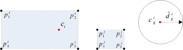
The initial positions of the network node, its goal and an obstacle; time step t k
$$ \forall_{O_{j},j = 1,\ldots,M} \quad \mathbf{c}^{i}_{(k+1)} \cap Vol\left(P^{j}_{(k)}\right) = \emptyset, $$(28)$$ \Delta t \cdot v^{i}_{max} \geq \left\|\mathbf{c}^{i}_{(k+1)} - \mathbf{c}^{i}_{(k)}\right\|. $$(29)The results of calculations are presented in Fig. 7.
Figure 7 
The calculated position of the reference point \(\mathbf {c}^{i}_{(k+1)}\) for the time step t k+1
-
Step 2: Calculate in the time step t k the displacement for all points from the set \(P^{i}_{(k)}\), solving the optimization problem for the estimated value of the reference distance \(\hat {d}_{g,(k+1)}^{i}\), and under the assumption that the point \(\mathbf {c}^{i}_{(k+1)}\) calculated in step 1 is fixed:
$$ \min_{P^{i}_{(k+1)}}\left[\sum_{\mathbf{p}^{i}_{a},\mathbf{p}^{i}_{b} \in P^{i},a\neq b}\left(\bar{r}_{a,b}^{i} - \left\|\mathbf{p}^{i}_{a,(k+1)} - \mathbf{p}^{i}_{b,(k+1)}\right\| \right)^{2} \right], $$(30)$$ \forall_{O_{j},j = 1,\ldots,M} \quad Vol\left(P^{i}_{(k+1)}\right) \cap Vol\left(P^{j}_{(k)}\right) = \emptyset. $$(31)The results of calculations are presented in Fig. 8.
Figure 8 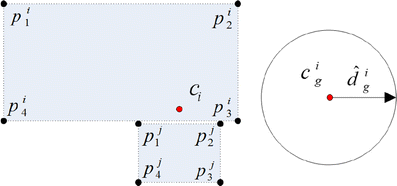
The calculated positions of points P i for the time step t k+1
-
Step 3: Recalculate the position of \(\mathbf {c}^{i}_{(k+1)}\) to satisfy the constraint on a solid body, and under the assumption that all points from the set \(P^{i}_{(k+1)}\) calculated in step 2 are fixed:
$$ \min_{c^{i}_{(k+1)}}\left[\sum_{\mathbf{p}^{i}_{a} \in P^{i},\mathbf{c}^{i} \in P^{i}}\left(\bar{r}_{0,a}^{i} - \left\|\mathbf{p}^{i}_{a,(k+1)} - \mathbf{c}^{i}_{(k+1)}\right\| \right)^{2} \right], $$(32)$$ \forall_{O_{j},j = 1,\ldots,M} \quad \mathbf{c}^{i}_{(k+1)} \cap Vol\left(P^{j}_{(k)}\right) = \emptyset, $$(33)The results of calculations are presented in Fig. 9.
Figure 9 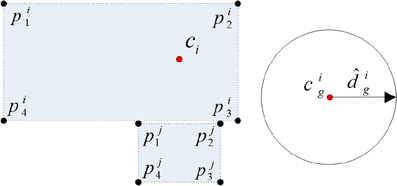
The final position of the reference point \(\mathbf {c}^{i}_{(k+1)}\) in the time step t k+1


The method of steepest descent is used to solve all above optimization problems. Finally, the device D i is moved to the designated location, which is recalculated again after the time interval Δ t.
5 Motion pattern computing for coherent network
To managing the mobility of a whole network and meet the requirements for providing continuous connectivity with a base station we propose two-level scheme for motion trajectories computing for all network nodes. Hence, calculations are carried out by two types of units, i.e., a base station (central unit in the system) and network nodes. The base station initiates the calculation process using the algorithm COHERENT_NET.
Algorithm COHERENT_NET: The coherent network design.
-
L1
The central station determines the initial position of each node in a network system based on the measurements from GPS or other localization systems described in [13]. Next, the messages with initial goals are distributed among nodes. Due to dynamic changes in a workspace the goals can change over time. In case of any changes new target points are transmitted to given nodes of a network.
-
L2
In the time step t k every mobile device (network node) computes its new position in the workspace using algorithm NETWORK_NODE, and next move to the designated location. The calculations are repeated every time interval Δ t due to changes in communication conditions and a workspace.
Algorithm NETWORK_NODE: Computing of the new position of a node D i expected in the time step t k+1 based on data measurements from the time t k .
-
step 1:
Read the data from the base station (current position and current goals).
-
step 2:
Calculate \(\hat {d}^{i}_{g,(k+1)}\), g = 1,…,J i – the distances between a node i and each its goal \(G_{g}^{i}\) expected after network transformation (in t k+1 = t k +Δ t) due to the formula (23).
-
step 3:
Calculate the displacements for points c i, and \(\mathbf {p}^{i}_{l}\), l = 1,…,L i solving in sequence three optimization problems: (27)–(29), (30)–(31) and (32)–(33).
-
step 4:
Move points c i and \(\mathbf {p}^{i}_{l}\), l = 1,…,L i to the new positions using results of step 3.
-
step 5:
Broadcast the new position of D i , update the time step (t k = t k +Δ t), and return to step 1.
The formation process of a simple network consisting of three nodes within transmission range is presented in Fig. 10.

The simple coherent network formation (initial, temporal and final topologies)
6 Case study results
We evaluated our mobility model through simulations. All experiments were performed using the software system for ad hoc network simulation on multiprocessor machines, described in [12,17]. In this paper we present and discuss the usage of our mobility model to design three ad hoc systems, starting from simple synthetic networks to more complex and realistic ones.
6.1 The design of coherent network
The first experiment presents the process of forming a cooperative and coherent network that enables the continuous communication with the base station. Let us assume the situation when the wireless mobile devices are grouped into three overlapping clusters. The communication between every pair of devices in a given cluster is assured. Moreover, the communication between all neighboring clusters is guaranteed. We can apply our mobility model to create a network with required characteristics. The network formation process – temporal and final results of our algorithm COHERENT_NET application is presented in Fig. 11.

Initial, temporal and final network topologies
6.2 Re-establishing the communication infrastructure
Let us consider a following emergency situation – an explosion at a petrol station has caused environmental damage and initiated a fire at a nearby factory (Fig. 12). Moreover, the fixed communication infrastructure in a disaster scene has been damaged. The goal is to support the rescue teams that are working in this area. It is obvious that the management of emergency activities such as guiding people out of dangerous areas and coordinating rescue teams requires permanent communication with the central operator. To establish the new communication channels a wireless mobile network can be used. In presented case study we consider the possibility of application of the COHERENT_NET algorithm to design a cooperative and coherent network supporting the coordination of the rescue mission. The goal is to create a wireless network with minimal number of nodes that ensue the connection between all rescue teams and the central station. The network composed of four rescue teams and seven mobile devices was used for establishing the communication in outdoor workspace. The result of the application of our algorithm for motion pattern calculation – the final network topology – is presented in Fig. 12.

The cooperative and coherent network for supporting a rescue mission
6.3 Emergency situation awareness
A wireless network formed by the mobile devices can reduce lack of situation awareness in areas prone to emergencies, and support the management of emergency activities. The network nodes that are free to move and organize themselves can gather data from many sources and transmit them to the central dispatcher. In presented case study we focus on emergency situation at the airport. Let us consider the following scenario – the monitoring system at the arrival hall was destroyed, and there is a suspicion of terrorist attack. In order to ensure the safety of people their activity should be monitored. We can create a wireless self-organizing network formed by mobile robots equipped with radio transceivers (IEEE 802.15.4) infrared cameras or motion sensors for on-line monitoring. These devices can identify people in their range and distribute sensing data to the crisis center. The attention should be focused on doors and popular transitions to other parts of the airport. Moreover, the devices should not be placed in the areas where they could hamper the normal traffic at the airport (green circles in Fig. 13).

The plan of the workspace (the arrival hall at the airport)
We performed a simulation experiment. The goal was to create the coherent IEEE 802.15.4 based wireless network for on-line monitoring of the arrival hall (90m ×90m). The plan of the arrival hall is presented in Fig. 13. The network was composed of 22 mobile devices calculating their motion patterns due to the COHERENT_NET algorithm. Fig. 14 presents the initial topology of the network. The results of the simulation of 200 seconds of network formation process are presented in Fig. 15 and in Table 1. From these results we can see that the final topology of the network is close to the expected one (most nodes reached their targets). However, the number of nodes assumed in this experiment was too small to create the optimal topology and satisfy all constraints.

The initial network topology

The final network topology
7 Conclusion
In this paper, we focused on mobility modeling in indor and outdoor scenarios and proposed a novel approach to cooperative mobile network design. Our approach combines techniques based on the potential field and the particle-based scheme for the motion paths computation. We defined the artificial potential function that is used in calculation of the optimal inter-node distances in a cooperative network. The main result of our research is the algorithm for designing and managing the mobility of ad hoc networks. The algorithm was implemented in our simulation platform and verified in many tests. In our opinion the presented mobility model is a good compromise between accuracy of the mobility modeling and computational burden. The presented case studies show that the COHERENT_NET algorithm can be successfully applied to design self-configuring, cooperative and coherent real life networks. In the future work, we plan to evaluate the performance of the COHERENT_NET algorithm in the testbed of middle-size ad hoc network in our laboratory.
References
Allen MP (2004) Introduction to molecular dynamics simulation. Computational soft matter: from synthetic polymers to proteins. Lect Notes23: 1–28.
Aravind A, Tahir H (2010) Towards modeling realistic mobility for performance evaluations in MANET. In: Proc. of the 9th international conference on adhoc mobile and wireless networks. pp 109–122.
Bai F, Sadagopan N, Helmy A (2003) IMPORTANT: a framework of systematically analyze the impact of mobility on performance of routing protocols for ad hoc networks. In: Proceedings of INFOCOM vol 2, San Francisco, pp 825–835.
Basagni S, Conti M, Giordano S, Stojmenovic I (2004) Mobile ad hoc networking. Wiley-Interscience IEEE Press.
Choset H, Lynch KM, Hutchinson S, Kantor G, Burgard W, Kavraki LE, Thrun S (2005) Principles of robot motion. The MIT Press, Cambridge.
Fongen A, Gjellerud M, Winjum E (2009) A military mobility model for manet research. In: Proceedings of IASTED international conference on parallel and distributed computing and networks.
Grossglauser M, Tse D (2001) Mobility increases the capacity of ad-hoc wireless networks. In: Proceedings of IEEE Infocom’01.
Kołodziej J, Khan SU, Wang L, Min-Allah N, Madani SA, Ghani N, Li H (2011) An application of markov jump process model for activity-based indoor mobility prediction in wireless networks. In: 9th IEEE international conference on frontiers of information technology (FIT). Islamabad, pp 51–56.
Musolesi M, Mascolo C (2009) Mobility models for systems evaluation. A survey. State of the art on middleware for network eccentric and mobile applications (MINEMA). Springer.
Mostafi Y (2011) Compressive sensing on mobile computing. IEEE Trans Mob Comput10(10): 1769–1784.
Niewiadomska-Szynkiewicz E, Sikora A (2011) Simulation-based design of self-organising and cooperative networks. Int J Space Based Situated Comput1(1): 68–75.
Niewiadomska-Szynkiewicz E, Sikora A (2012) A software tool for federated simulation of wireless sensor networks and mobile ad hoc networks. In: Jonasson K (ed) Applied parallel scientific computing, LNCS7133, part I. Springer-Verlag, pp 303–313.
Niewiadomska-Szynkiewicz E (2012) Localization in wireless sensor networks: classification and evaluation of techniques, University of Zielona Gora Press. Int J of App Math Comput Sci22(2): 281–297.
Rapaport DC (1996) The art of molecular dynamics simulation. Cambridge University Press, New York.
Rappaport TS (2009) Wireless communications. Principles and practice. Prentice Hall, USA.
Roy RR (2010) Handbook of mobile ad hoc networks for mobility models. Springer, USA.
Sikora A, Niewiadomska-Szynkiewicz E (2009) A parallel and distributed simulation of ad hoc networks. J Telecomm Inf Technol3: 76–84.
Singh S (2002) Liquid crystals. fundamentals. World Scientific Publishing Co. Pte. Ltd, Singapore.
Szynkiewicz W, Blaszczyk J (2011) Optimization-based approach to path planning for closed-chain robot systems. Int J Appl Math Comput Sci21(4): 659–67.
Acknowledgments
This work was partially supported by National Science Centre grant NN514 672940.
Author information
Authors and Affiliations
Corresponding author
Rights and permissions
Open Access This article is distributed under the terms of the Creative Commons Attribution 2.0 International License (https://creativecommons.org/licenses/by/2.0), which permits unrestricted use, distribution, and reproduction in any medium, provided the original work is properly cited.
About this article
Cite this article
Niewiadomska-Szynkiewicz, E., Sikora, A. & Kołodziej, J. Modeling Mobility in Cooperative Ad Hoc Networks. Mobile Netw Appl 18, 610–621 (2013). https://doi.org/10.1007/s11036-013-0450-2
Published:
Issue Date:
DOI: https://doi.org/10.1007/s11036-013-0450-2