Local Convergence Properties of Douglas–Rachford and Alternating Direction Method of Multipliers

Abstract

The Douglas–Rachford and alternating direction method of multipliers are two proximal splitting algorithms designed to minimize the sum of two proper lower semi-continuous convex functions whose proximity operators are easy to compute. The goal of this work is to understand the local linear convergence behaviour of Douglas–Rachford (resp. alternating direction method of multipliers) when the involved functions (resp. their Legendre–Fenchel conjugates) are moreover partly smooth. More precisely, when the two functions (resp. their conjugates) are partly smooth relative to their respective smooth submanifolds, we show that Douglas–Rachford (resp. alternating direction method of multipliers) (i) identifies these manifolds in finite time; (ii) enters a local linear convergence regime. When both functions are locally polyhedral, we show that the optimal convergence radius is given in terms of the cosine of the Friedrichs angle between the tangent spaces of the identified submanifolds. Under polyhedrality of both functions, we also provide conditions sufficient for finite convergence. The obtained results are illustrated by several concrete examples and supported by numerical experiments.

Appendices

Appendix A: Proof of Theorem 4.1

We start with the following lemma which is needed in the proof of Theorem 4.1.

Lemma A.1

Suppose that conditions (H.2) and (H.3) hold, and that $\gamma _k$ is convergent. Then

$$\begin{aligned} \lim _{k\rightarrow +\infty } \gamma _k = \gamma . \end{aligned}$$

Proof

Since $\gamma _k$ is convergent, it has a unique cluster point, say $\lim _{k \rightarrow +\infty } \gamma _k = \gamma '$. It is then sufficient to show that $\gamma '=\gamma$. Suppose that $\gamma ' \ne \gamma$. Fix some $\varepsilon \in ]0,{|} \gamma '-\gamma {|}[$. Thus, there exist an index $K > 0$ such that for all $k \ge K$,

$$\begin{aligned} {|} \gamma _k-\gamma ' {|} < \varepsilon /2 . \end{aligned}$$

Therefore

$$\begin{aligned} {|} \gamma _k-\gamma {|} \ge {|} \gamma '-\gamma {|} - {|} \gamma _k-\gamma ' {|} > \varepsilon /2 . \end{aligned}$$

It then follows that

$$\begin{aligned} \lambda _k(2-\lambda _k)\varepsilon \le 2\lambda _k\varepsilon \le 4\lambda _k{|} \gamma _k-\gamma {|} . \end{aligned}$$

Denote $\overline{\tau } :=\sup _{k \mathbb {N}}\lambda _k(2-\lambda _k)$ which is obviously positive and bounded since $\lambda _k \in [0,2]$. Summing both sides for $k \ge K$ we get

$$\begin{aligned} \begin{aligned} \varepsilon \mathbin {{\sum }}_{k \in \mathbb {N}} \lambda _k(2-\lambda _k) - K\overline{\tau } \le \varepsilon \sum _{k=K}^{+\infty } \lambda _k(2-\lambda _k) \le 4\sum _{k \in \mathbb {N}} \lambda _k {|} \gamma _k-\gamma {|} , \end{aligned} \end{aligned}$$

which, in view of (H.3), implies

$$\begin{aligned} \sum _{k \in \mathbb {N}} \lambda _k(2-\lambda _k) \le \varepsilon ^{-1}(\lambda _k {|} \gamma _k-\gamma {|} + K\overline{\tau }) < +\infty , \end{aligned}$$

leading to a contradiction with (H.2). $\square$

Proof

(Theorem 4.1) To prove our claim, we only need to check the conditions listed in [3, Theorem 4].

• (i) As (A.3) assumes the set of minimizers of $({\mathcal {P}})$ is non-empty, so is the set $\mathrm {Fix}(\mathscr {F}_{\gamma })$, since the former is nothing but $\mathrm {prox}_{\gamma J}(\mathrm {Fix}(\mathscr {F}_{\gamma }))$ [20, Proposition 25.1(ii)].

• (ii) Since $\mathscr {F}_{\gamma _k}$ is firmly non-expansive by Lemma 2.2, $\mathscr {F}_{\gamma _k,\lambda _k}$ is $\frac{\lambda _k}{2}$-averaged non-expansive, hence non-expansive, owing to Lemma 2.1(iiii).

• (iii) Let $\rho \in [0,+\infty [$ and $z \in \mathbb {R}^n$ such that ${||} z {||} \le \rho$, Then we have

  $$\begin{aligned} \begin{aligned} (\mathscr {F}_{\gamma _k}- \mathscr {F}_{\gamma }) (z)&=\tfrac{\mathrm {rprox}_{\gamma _k G}\circ \mathrm {rprox}_{\gamma _k J}}{2}(z) - \tfrac{\mathrm {rprox}_{\gamma G}\circ \mathrm {rprox}_{\gamma J}}{2}(z) \\&=\left( {\tfrac{\mathrm {rprox}_{\gamma _k G}\circ \mathrm {rprox}_{\gamma _k J}}{2}(z) - \tfrac{\mathrm {rprox}_{\gamma _k G}\circ \mathrm {rprox}_{\gamma J}}{2}(z)}\right) \\&- \left( {\tfrac{\mathrm {rprox}_{\gamma G}\circ \mathrm {rprox}_{\gamma J}}{2}(z) - \tfrac{\mathrm {rprox}_{\gamma _k G}\circ \mathrm {rprox}_{\gamma J}}{2}(z)}\right) \\&=\left( {\tfrac{\mathrm {rprox}_{\gamma _k G}\circ \mathrm {rprox}_{\gamma _k J}}{2}(z) - \tfrac{\mathrm {rprox}_{\gamma _k G}\circ \mathrm {rprox}_{\gamma J}}{2}(z)}\right) \\&- \left( {\mathrm {prox}_{\gamma G}\circ \mathrm {rprox}_{\gamma J}(z) - \mathrm {prox}_{\gamma _k G}\circ \mathrm {rprox}_{\gamma J}(z)}\right) . \end{aligned} \end{aligned}$$

  Thus, by virtue of Lemma 2.1(iii), we have

  $$\begin{aligned} {||} (\mathscr {F}_{\gamma _k}- \mathscr {F}_{\gamma }) (z) {||}&\le {||} \mathrm {prox}_{\gamma _k J}(z) - \mathrm {prox}_{\gamma J}(z) {||}\\&\quad +{||} \mathrm {prox}_{\gamma _k G}(\mathrm {rprox}_{\gamma J}(z)) - \mathrm {prox}_{\gamma G}(\mathrm {rprox}_{\gamma J}(z)) {||} . \end{aligned}$$

  Let’s bound the first term. From the resolvent equation [41], and Lemma 2.1(i) (ii) (v), we have

  

  (24)

  With similar arguments, we also obtain

  

  (25)

  Combining (24) and (25) leads to

  

  (26)

  whence we get

  

  Therefore, from (H.3), we deduce that

  $$\begin{aligned} \left\{ \sup _{{||} z {||} \le \rho } {||} (\mathscr {F}_{\gamma _k,\lambda _k}- \mathscr {F}_{\gamma ,\lambda _k}) (z) {||}_{k \in \mathbb {N}}\right\} \in \ell _{+}^1 . \end{aligned}$$

In other words, the non-stationary iteration (7) is a perturbed version of the stationary one (4) with an error term which is summable thanks to (H.3). The claim on the convergence of ${z}^\star$ follows by applying [24, Corollary 5.2]. Moreover, $x^{\star }:=\mathrm {prox}_{\gamma J}({z}^\star )$ is a solution of $({\mathcal {P}})$. In turn, using non-expansiveness of $\mathrm {prox}_{\gamma _k J}$ and (24), we have

$$\begin{aligned} {||} x_{k}- x^{\star } {||} \le {||} {z}_{k}- {z}^\star {||} + \frac{{|} \gamma _k - \gamma {|}}{\gamma }({||} {z}^\star {||} + {||} \mathrm {prox}_{\gamma J}(0) {||}) , \end{aligned}$$

and thus, the right-hand side goes to zero as $k \rightarrow +\infty$ as we are in finite dimension and since $\gamma _k \rightarrow \gamma$ owing to Lemma A.1. This entails that the shadow sequence $\{x_{k}\}_{k \in \mathbb {N}}$ also converges to $x^{\star }$. With similar arguments, we can also show that $\{v_{k}\}_{k \in \mathbb {N}}$ converges to $x^{\star }$ (using, for instance, (25) and non-expansiveness of $\mathrm {prox}_{\gamma _k G}$). $\square$

Appendix B: Proofs of Section 5

Proof

(Theorem 5.1) By Theorem 4.1, all the sequences generated by (6) converge, i.e.

$$\begin{aligned} {z}_{k}\rightarrow {z}^\star \in \mathrm {Fix}(\mathscr {F}_{\gamma ,\lambda }),\quad x_{k}, v_{k}, \rightarrow x^{\star }= \mathrm {prox}_{\gamma J}({z}^\star ) \in \mathrm {Argmin}(G+J). \end{aligned}$$

The non-degeneracy condition (ND) is equivalent to

(27)

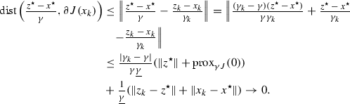
• (i) The update of $x_{k+1}$ and $v_{k+1}$ in iteration (6) is equivalent to the monotone inclusions

  

  It then follows that

  

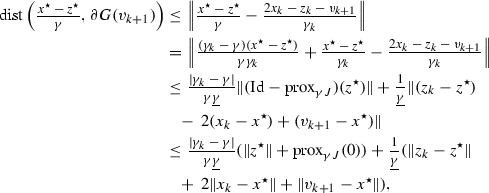
  and the right-hand side converges to 0 in view of Theorem 4.1 and Lemma A.1. Similarly, we have

  

  By assumption, $G, J \in \Gamma _0(\mathbb {R}^n)$, hence are subdifferentially continuous at every point in their respective domains [32, Example 13.30], and in particular at $x^{\star }$. It then follows that $G(v_{k}) \rightarrow G(x^{\star })$ and $J(x_{k}) \rightarrow J(x^{\star })$. Altogether, this shows that the conditions of [42, Theorem 5.3] are fulfilled for G and J, and the finite identification claim follows.

• (ii)

  • (a) In this case, $\mathcal {M}^{J}_{x^{\star }}$ is an affine subspace, i.e. $\mathcal {M}^{J}_{x^{\star }}= x^{\star }+{T_{x^{\star }}^{J}}$. Since J is partly smooth at $x^{\star }$ relative to $\mathcal {M}^{J}_{x^{\star }}$, the sharpness property holds at all nearby points in $\mathcal {M}^{J}_{x^{\star }}$ [9, Proposition 2.10]. Thus for k large enough, i.e. $x_{k}$ sufficiently close to $x^{\star }$ on $\mathcal {M}^{J}_{x^{\star }}$, we have indeed $\mathcal {T}_{x_{k}}(\mathcal {M}^{J}_{x^{\star }})={T_{x^{\star }}^{J}}={T_{x_{k}}^{J}}$ as claimed.

  • (b) Similar to (ii)(a).

  • (c) It is immediate to verify that a locally polyhedral function around $x^{\star }$ is indeed partly smooth relative to the affine subspace $x^{\star }+{T_{x^{\star }}^{J}}$, and thus, the first claim follows from (ii)(a). For the rest, it is sufficient to observe that by polyhedrality, for any $x \in \mathcal {M}^{J}_{x^{\star }}$ near $x^{\star }$, $\partial J(x) = \partial J(x^{\star })$. Therefore, combining local normal sharpness [9, Proposition 2.10] and Lemma 5.1 yields the second conclusion.

  • (d) Similar to (ii)(c). $\square$

Proof

(Proposition 5.1) From (7), we have

$$\begin{aligned} {z}_{k+1}= \mathscr {F}_{\gamma ,\lambda _k}({z}_{k}) + e_k \end{aligned}$$

where $\{{||} e_k {||}\}_{k \in \mathbb {N}} = \{O(\lambda _k{|} \gamma _k-\gamma {|})\}_{k \in \mathbb {N}} \in \ell _+^1$ (see the proof of Theorem 4.1). Since $\mathscr {F}_{\gamma _k}$ is firmly non-expansive by Lemma 2.2, $\mathscr {F}_{\gamma ,\lambda _k}$ is $\frac{\lambda _k}{2}$-averaged non-expansive owing to Lemma 2.1(iiii). Thus arguing as in the proof of [24, Theorem 3.1], we have

$$\begin{aligned} \begin{aligned} {||} {z}_{k}-{z}^\star {||}^2&\le {||} \mathscr {F}_{\gamma ,\lambda _k}({z}_{k-1})-\mathscr {F}_{\gamma ,\lambda _k}({z}^\star ) {||}^2 + C {||} e_{k-1} {||}\\&\le {||} \mathscr {F}_{\gamma ,\lambda _k}({z}_{k-1})-\mathscr {F}_{\gamma ,\lambda _k}({z}^\star ) {||}^2 - \tfrac{2-\lambda _{k-1}}{\lambda _{k-1}}{||} {z}_{k}-{z}_{k-1} {||}^2 + C {||} e_{k-1} {||}\\&\le {||} {z}_{k-1}- {z}^\star {||}^2 - \tau _{k-1}{||} v_{k}- x_{k-1} {||}^2 + C {||} e_{k-1} {||}, \end{aligned} \end{aligned}$$

where $C < +\infty$ by boundedness of ${z}_{k}$ and $e_k$. Let $g_k=({z}_{k-1}-x_{k-1})/\gamma _{k-1}$ and $h_k=(2x_{k-1}-{z}_{k-1}-v_{k})/\gamma _{k-1}$. By definition, we have $(g_k,h_k) \in \partial J(x_{k-1}) \times \partial G(v_{k})$. Suppose that neither $\mathcal {M}^{J}_{x^{\star }}$ nor $\mathcal {M}^{G}_{x^{\star }}$ have been identified at iteration k. That is $x_{k-1}\notin \mathcal {M}^{J}_{x^{\star }}$ and $v_{k}\notin \mathcal {M}^{G}_{x^{\star }}$, and by assumption, $g_k \in \mathrm {rbd}(\partial J(x^{\star }))$ and $h_k \in \mathrm {rbd}(\partial G(x^{\star }))$, which implies that $g_k+h_k=(v_{k}-x_{k-1})/\gamma _{k-1} \in \mathrm {rbd}(\partial J(x^{\star })) + \mathrm {rbd}(\partial G(x^{\star }))$. Thus, the above inequality becomes

$$\begin{aligned}&{||} {z}_{k}-{z}^\star {||}^2\nonumber \\&\quad \le {||} {z}_{k-1}- {z}^\star {||}^2 - \gamma _{k-1}^2\tau _{k-1}\mathrm {dist}\big ({0,\mathrm {rbd}(\partial J(x^{\star })) + \mathrm {rbd}(\partial G(x^{\star }))}\big )^2 + C {||} e_{k-1} {||} \\&\quad \le {||} {z}_{k-1}- {z}^\star {||}^2 - \gamma _{k-1}^2\tau _{k-1}\mathrm {dist}\big ({0,\mathrm {rbd}(\partial J(x^{\star })+\partial G(x^{\star }))}\big )^2 + C {||} e_{k-1} {||} \\&\quad \le {||} z_0 - {z}^\star {||}^2 - k \underline{\gamma }^2\underline{\tau }\mathrm {dist}\big ({0,\mathrm {rbd}(\partial J(x^{\star })+\partial G(x^{\star }))}\big )^2 + O\big ({\mathbin {{\sum }}_{k \in \mathbb {N}} \lambda _k{|} \gamma _k-\gamma {|}}\big ), \end{aligned}$$

and $\mathrm {dist}\big ({0,\mathrm {rbd}(\partial J(x^{\star })+\partial G(x^{\star }))}\big ) > 0$ owing to condition (ND). Taking k as the largest integer such that the bound in the right hand is positive, we deduce that the number of iterations where both $\mathcal {M}^{J}_{x^{\star }}$ and $\mathcal {M}^{G}_{x^{\star }}$ have not been identified yet does not exceed the claimed bound (8). Thus, finite identification necessarily occurs at some k larger than this bound. $\square$

Appendix C: Proofs of Section 6

1.1 Riemannian Geometry

Let $\mathcal {M}$ be a $C^2$-smooth embedded submanifold of $\mathbb {R}^n$ around a point x. With some abuse of terminology, we shall state $C^2$-manifold instead of $C^2$-smooth embedded submanifold of $\mathbb {R}^n$. The natural embedding of a submanifold $\mathcal {M}$ into $\mathbb {R}^n$ permits to define a Riemannian structure and to introduce geodesics on $\mathcal {M}$, and we simply say $\mathcal {M}$ is a Riemannian manifold. We denote respectively $\mathcal {T}_{\mathcal {M}}(x)$ and $\mathcal {N}_{\mathcal {M}}(x)$ the tangent and normal space of $\mathcal {M}$ at point near x in $\mathcal {M}$.

Exponential map

Geodesics generalize the concept of straight lines in $\mathbb {R}^n$, preserving the zero acceleration characteristic, to manifolds. Roughly speaking, a geodesic is locally the shortest path between two points on $\mathcal {M}$. We denote by $\mathfrak {g}(t;x, h)$ the value at $t \in \mathbb {R}$ of the geodesic starting at $\mathfrak {g}(0;x,h) = x \in \mathcal {M}$ with velocity (which is uniquely defined). For every $h \in \mathcal {T}_{\mathcal {M}}(x)$, there exists an interval I around 0 and a unique geodesic $\mathfrak {g}(t;x, h): I \rightarrow \mathcal {M}$ such that $\mathfrak {g}(0; x, h) = x$ and $\dot{\mathfrak {g}}(0;x, h) = h$. The mapping

$$\begin{aligned} \mathrm {Exp}_x : \mathcal {T}_{\mathcal {M}}(x) \rightarrow \mathcal {M},\quad h\mapsto \mathrm {Exp}_{x}(h) = \mathfrak {g}(1;x, h) , \end{aligned}$$

is called Exponential map. Given $x, x' \in \mathcal {M}$, the direction $h \in \mathcal {T}_{\mathcal {M}}(x)$ we are interested in is such that $\mathrm {Exp}_x(h) = x' = \mathfrak {g}(1;x, h)$.

Parallel translation

Given two points $x, x' \in \mathcal {M}$, let $\mathcal {T}_{\mathcal {M}}(x), \mathcal {T}_{\mathcal {M}}(x')$ be their corresponding tangent spaces. Define $\tau : \mathcal {T}_{\mathcal {M}}(x) \rightarrow \mathcal {T}_{\mathcal {M}}(x')$ the parallel translation along the unique geodesic joining x to $x'$, which is isomorphism and isometry w.r.t. the Riemannian metric.

Riemannian gradient and Hessian

For a vector $v \in \mathcal {N}_{\mathcal {M}}(x)$, the Weingarten map of $\mathcal {M}$ at x is the operator $\mathfrak {W}_{x}(\cdot , v): \mathcal {T}_{\mathcal {M}}(x) \rightarrow \mathcal {T}_{\mathcal {M}}(x)$ defined by $\mathfrak {W}_{x}(\cdot , v) = - \mathrm {P}_{\mathcal {T}_{\mathcal {M}}(x)} \mathrm {d} V[h]$, where V is any local extension of v to a normal vector field on $\mathcal {M}$. The definition is independent of the choice of the extension V, and $\mathfrak {W}_{x}(\cdot , v)$ is a symmetric linear operator which is closely tied to the second fundamental form of $\mathcal {M}$; see [43, Proposition II.2.1].

Let G be a real-valued function which is $C^2$ along the $\mathcal {M}$ around x. The covariant gradient of G at $x' \in \mathcal {M}$ is the vector $\nabla _{\mathcal {M}} G(x') \in \mathcal {T}_{\mathcal {M}}(x')$ defined by

where $\mathrm {P}_{\mathcal {M}}$ is the projection operator onto $\mathcal {M}$.

The covariant Hessian of G at $x'$ is the symmetric linear mapping $\nabla ^2_{\mathcal {M}} G(x')$ from $\mathcal {T}_{\mathcal {M}}(x')$ to itself which is defined as

(28)

This definition agrees with the usual definition using geodesics or connections [44]. Now assume that $\mathcal {M}$ is a Riemannian embedded submanifold of $\mathbb {R}^{n}$ and that a function G has a $C^2$-smooth restriction on $\mathcal {M}$. This can be characterized by the existence of a $C^2$-smooth extension (representative) of G, i.e. a $C^2$-smooth function $\widetilde{G}$ on $\mathbb {R}^{n}$ such that $\widetilde{G}$ agrees with G on $\mathcal {M}$. Thus, the Riemannian gradient $\nabla _{\mathcal {M}}G(x')$ is also given by

$$\begin{aligned} \nabla _{\mathcal {M}} G(x') = \mathrm {P}_{\mathcal {T}_{\mathcal {M}}(x')} \nabla \widetilde{G}(x') , \end{aligned}$$

(29)

and $\forall h \in \mathcal {T}_{\mathcal {M}}(x')$, the Riemannian Hessian reads

$$\begin{aligned} \begin{aligned} \nabla ^2_{\mathcal {M}} G(x') h&= \mathrm {P}_{\mathcal {T}_{\mathcal {M}}(x')} \mathrm {d} (\nabla _{\mathcal {M}} G)(x')[h] = \mathrm {P}_{\mathcal {T}_{\mathcal {M}}(x')} \mathrm {d} \big ({ x' \mapsto \mathrm {P}_{\mathcal {T}_{\mathcal {M}}(x')} \nabla _{\mathcal {M}} \widetilde{G} }\big )[h] \\&= \mathrm {P}_{\mathcal {T}_{\mathcal {M}}(x')} \nabla ^2 \widetilde{G}(x') h + \mathfrak {W}_{x'}\big ({h, \mathrm {P}_{\mathcal {N}_{\mathcal {M}}(x')}\nabla \widetilde{G}(x')}\big ) , \end{aligned}\nonumber \\ \end{aligned}$$

(30)

where the last equality comes from [45, Theorem 1]. When $\mathcal {M}$ is an affine or linear subspace of $\mathbb {R}^{n}$, then obviously $\mathcal {M}= x + \mathcal {T}_{\mathcal {M}}(x)$, and $\mathfrak {W}_{x'}(h, \mathrm {P}_{\mathcal {N}_{\mathcal {M}}(x')} \nabla \widetilde{G}(x')) = 0$, hence (30) reduces to $\nabla ^2_{\mathcal {M}} G(x') = \mathrm {P}_{\mathcal {T}_{\mathcal {M}}(x')} \nabla ^2 \widetilde{G}(x') \mathrm {P}_{\mathcal {T}_{\mathcal {M}}(x')}$. See [43, 46] for more materials on differential and Riemannian manifolds.

We have the following proposition characterizing the parallel translation and the Riemannian Hessian of two close points in $\mathcal {M}$.

LemmaC.1

Let $x, x'$ be two close points in $\mathcal {M}$, denote $\mathcal {T}_{\mathcal {M}}(x), \mathcal {T}_{\mathcal {M}}(x')$ be the tangent spaces of $\mathcal {M}$ at $x, x'$, respectively, and $\tau : \mathcal {T}_{\mathcal {M}}(x') \rightarrow \mathcal {T}_{\mathcal {M}}(x)$ be the parallel translation along the unique geodesic joining from x to $x'$, then for the parallel translation we have, given any bounded vector $v \in \mathbb {R}^{n}$

$$\begin{aligned} (\tau \mathrm {P}_{\mathcal {T}_{\mathcal {M}}(x')} - \mathrm {P}_{\mathcal {T}_{\mathcal {M}}(x)}) v = o(v) . \end{aligned}$$

(31)

The Riemannian Taylor expansion of $J \in C^2(\mathcal {M})$ at x for $x'$ reads,

$$\begin{aligned} \tau \nabla _{\mathcal {M}} J(x') = \nabla _{\mathcal {M}} J(x) + \nabla ^2_{\mathcal {M}} J(x)\mathrm {P}_{\mathcal {T}_{\mathcal {M}}(x)}(x'-x) + o(x'-x) . \end{aligned}$$

(32)

Proof

See [30, Lemma B.1 and B.2]. $\square$

Proof

(Proposition 6.1) Since $W_{\overline{{G}}}, W_{\overline{{J}}}$ are both firmly non-expansive by Lemma 6.1, it follows from [20, Example 4.7] that ${M}_{\overline{{G}}}$ and ${M}_{\overline{{J}}}$ are firmly non-expansive. As a result, M is firmly non-expansive [20, Proposition 4.21(i)–(ii)], and equivalently that $M_\lambda$ is $\frac{\lambda }{2}$-averaged by Lemma 2.1(i)$\Leftrightarrow$(iiii).

Under the assumptions of Theorem 5.1, there exists $K \in \mathbb {N}$ large enough such that for all $k \ge K$, $(x_{k},v_{k}) \in \mathcal {M}^{J}_{x^{\star }}\times \mathcal {M}^{G}_{x^{\star }}$. Denote ${T_{x_{k}}^{J}}$ and ${T_{x^{\star }}^{J}}$ be the tangent spaces corresponding to $x_{k}$ and $x^{\star }\in \mathcal {M}^{J}_{x^{\star }}$, and similarly $T_{x_{k}}^G$ and $T_{x^{\star }}^G$ the tangent spaces corresponding to $v_{k}$ and $x^{\star }\in \mathcal {M}^{G}_{x^{\star }}$. Denote $\tau _{k}^{J} : {T_{x_{k}}^{J}} \rightarrow {T_{x^{\star }}^{J}}$ (resp. $\tau _{k}^{G} : T_{v_{k}}^G \rightarrow T_{x^{\star }}^G$) the parallel translation along the unique geodesic on $\mathcal {M}^{J}_{x^{\star }}$ (resp. $\mathcal {M}^{G}_{x^{\star }}$) joining $x_{k}$ to $x^{\star }$ (resp. $v_{k}$ to $x^{\star }$).

From (6), for $x_{k}$, we have

$$\begin{aligned} \left\{ \begin{aligned} x_{k}&= \mathrm {prox}_{\gamma _k J} ({z}_{k}) , \\ x^{\star }&= \mathrm {prox}_{\gamma J} ({z}^\star ) , \end{aligned} \right. \,\iff \left\{ \begin{aligned} {z}_{k}- x_{k}&\in \gamma _k \partial J(x_{k}) , \\ {z}^\star - x^{\star }&\in \gamma \partial J(x^{\star }) . \end{aligned} \right. \end{aligned}$$

Projecting on the corresponding tangent spaces, using Lemma 5.1, and applying the parallel translation operator $\tau _{k}^{J}$ lead to

$$\begin{aligned} \begin{aligned} \gamma _k \tau _{k}^{J} \nabla _{\mathcal {M}^{J}_{x^{\star }}} J(x_{k})&= \tau _{k}^{J} \mathrm {P}_{T_{x_{k}}^{J}} ({z}_{k}- x_{k}) = \mathrm {P}_{T_{x^{\star }}^{J}} ({z}_{k}- x_{k}) + \big ({\tau _{k}^{J} \mathrm {P}_{T_{x_{k}}^{J}} - \mathrm {P}_{T_{x^{\star }}^{J}}}\big ) ({z}_{k}- x_{k}) , \\ \gamma \nabla _{\mathcal {M}^{J}_{x^{\star }}} J(x^{\star })&= \mathrm {P}_{T_{x^{\star }}^{J}} ({z}^\star - x^{\star }) . \end{aligned} \end{aligned}$$

We then obtain

$$\begin{aligned} \gamma _k \tau _{k}^{J} \nabla _{\mathcal {M}^{J}_{x^{\star }}} J(x_{k}) - \gamma \nabla _{\mathcal {M}^{J}_{x^{\star }}} J(x^{\star })&= \gamma \tau _{k}^{J} \nabla _{\mathcal {M}^{J}_{x^{\star }}} J(x_{k}) - \gamma \nabla _{\mathcal {M}^{J}_{x^{\star }}} J(x^{\star }) \nonumber \\&\qquad + (\gamma _k-\gamma ) \tau _{k}^{J} \nabla _{\mathcal {M}^{J}_{x^{\star }}} J(x_{k}) \nonumber \\&= \mathrm {P}_{T_{x^{\star }}^{J}}\big ({({z}_{k}- {z}^\star ) - (x_{k}- x^{\star })}\big ) \nonumber \\&\qquad + \underset{\mathbf{Term 1 }}{\underbrace{\big ({\tau _{k}^{J} \mathrm {P}_{T_{x_{k}}^{J}} - \mathrm {P}_{T_{x^{\star }}^{J}}}\big ) ({z}_{k}- x_{k}-{z}^\star +x^{\star })}} \nonumber \\&\qquad + \underset{\mathbf{Term 2 }}{\underbrace{\big ({\tau _{k}^{J} \mathrm {P}_{T_{x_{k}}^{J}} - \mathrm {P}_{T_{x^{\star }}^{J}}}\big ) ({z}^\star - x^{\star })}} . \end{aligned}$$

(33)

For $(\gamma _k-\gamma ) \tau _{k}^{J} \nabla _{\mathcal {M}^{J}_{x^{\star }}} J(x_{k})$, since the Riemannian gradient $\nabla _{\mathcal {M}^{J}_{x^{\star }}} J(x_{k})$ is single-valued and bounded on bounded sets, we have

$$\begin{aligned} {||} (\gamma _k-\gamma ) \tau _{k}^{J} \nabla _{\mathcal {M}^{J}_{x^{\star }}} J(x_{k}) {||} = O({|} \gamma _k - \gamma {|}) . \end{aligned}$$

(34)

Combining (24) and (31), we have for Term 1

$$\begin{aligned} \begin{aligned} \left( \tau _{k}^{J} \mathrm {P}_{T_{x_{k}}^{J}} - \mathrm {P}_{T_{x^{\star }}^{J}}\right) ({z}_{k}- x_{k}-{z}^\star +x^{\star }) = o({z}_{k}-{z}^\star ) + o({|} \gamma _k - \gamma {|}) . \end{aligned} \end{aligned}$$

(35)

As far as Term 2 is concerned, with (13), (24) and the Riemannian Taylor expansion (32), we have

$$\begin{aligned}&\gamma \tau _{k}^{J} \nabla _{\mathcal {M}^{J}_{x^{\star }}} J(x_{k}) - \gamma \nabla _{\mathcal {M}^{J}_{x^{\star }}} J(x^{\star }) - \big ({\tau _{k}^{J} \mathrm {P}_{T_{x_{k}}^{J}} - \mathrm {P}_{T_{x^{\star }}^{J}}}\big ) ({z}^\star - x^{\star }) \nonumber \\&\quad = \tau _{k}^{J} \big ({\gamma \nabla _{\mathcal {M}^{J}_{x^{\star }}} J(x_{k}) - \mathrm {P}_{T_{x_{k}}^{J}} ({z}^\star - x^{\star })}\big ) - \big ({ \gamma \nabla _{\mathcal {M}^{J}_{x^{\star }}} J(x^{\star }) - \mathrm {P}_{T_{x^{\star }}^{J}} ({z}^\star - x^{\star }) }\big ) \nonumber \\&\quad = \tau _{k}^{J} \nabla _{\mathcal {M}^{J}_{x^{\star }}} \overline{{J}}(x_{k}) - \nabla _{\mathcal {M}^{J}_{x^{\star }}} \overline{{J}}(x^{\star }) = \mathrm {P}_{T_{x^{\star }}^{J}}\nabla ^2_{\mathcal {M}^{J}_{x^{\star }}} \overline{{J}}(x^{\star }) \mathrm {P}_{T_{x^{\star }}^{J}}(x_{k}-x^{\star }) + o(x_{k}-x^{\star }) \nonumber \\&\quad = \mathrm {P}_{T_{x^{\star }}^{J}}\nabla ^2_{\mathcal {M}^{J}_{x^{\star }}} \overline{{J}}(x^{\star }) \mathrm {P}_{T_{x^{\star }}^{J}}(x_{k}-x^{\star }) + o({z}_{k}-{z}^\star ) + o({|} \gamma _k - \gamma {|}). \end{aligned}$$

(36)

Therefore, inserting (34), (35) and (36) into (33), we obtain

$$\begin{aligned}&H_{\overline{{J}}} (x_{k}- x^{\star }) = \mathrm {P}_{T_{x^{\star }}^{J}}({z}_{k}- {z}^\star ) - \mathrm {P}_{T_{x^{\star }}^{J}}(x_{k}- x^{\star }) + o({z}_{k}- {z}^\star ) + O({|} \gamma _k - \gamma {|}) \nonumber \\&\quad \Rightarrow (\mathrm {Id}+ H_{\overline{{J}}}) \mathrm {P}_{T_{x^{\star }}^{J}}(x_{k}- x^{\star }) = \mathrm {P}_{T_{x^{\star }}^{J}}({z}_{k}- {z}^\star ) + o({z}_{k}- {z}^\star ) + O({|} \gamma _k - \gamma {|}) \nonumber \\&\quad \Rightarrow \mathrm {P}_{T_{x^{\star }}^{J}}(x_{k}- x^{\star }) = W_{\overline{{J}}} \mathrm {P}_{T_{x^{\star }}^{J}}({z}_{k}- {z}^\star ) + o({z}_{k}- {z}^\star ) + O({|} \gamma _k - \gamma {|}) \nonumber \\&\quad \Rightarrow \mathrm {P}_{T_{x^{\star }}^{J}}(x_{k}- x^{\star }) = \mathrm {P}_{T_{x^{\star }}^{J}}W_{\overline{{J}}} \mathrm {P}_{T_{x^{\star }}^{J}}({z}_{k}- {z}^\star ) + o({z}_{k}- {z}^\star ) + O({|} \gamma _k - \gamma {|}) \nonumber \\&\quad \Rightarrow x_{k}- x^{\star }= {M}_{\overline{{J}}}({z}_{k}- {z}^\star ) + o({z}_{k}- {z}^\star ) + O({|} \gamma _k - \gamma {|}) , \end{aligned}$$

(37)

where we used the fact that $x_{k}-x^{\star }= \mathrm {P}_{T_{x^{\star }}^{J}}(x_{k}-x^{\star }) + o(x_{k}-x^{\star })$ [47, Lemma 5.1].

Similarly for $v_{k+1}$, we have

$$\begin{aligned} \left\{ \begin{aligned} v_{k+1}&= \mathrm {prox}_{\gamma _k G}(2x_{k}- {z}_{k}) , \\ x^{\star }&= \mathrm {prox}_{\gamma G}(2x^{\star }- {z}^\star ) , \end{aligned} \right. \,\Longleftrightarrow \, \left\{ \begin{aligned} 2x_{k}- {z}_{k}- v_{k+1}&\in \gamma \partial J(v_{k+1}) , \\ 2x^{\star }- {z}^\star - x^{\star }&\in \gamma \partial J(x^{\star }) . \end{aligned} \right. \end{aligned}$$

Upon projecting onto the corresponding tangent spaces and applying the parallel translation $\tau _{k+1}^{G}$, we get

$$\begin{aligned} \begin{aligned} \gamma _k \tau _{k+1}^{G} \nabla _{\mathcal {M}^{G}_{x^{\star }}} G(v_{k+1})&= \tau _{k+1}^{G} \mathrm {P}_{T_{v_{k+1}}^{G}} (2x_{k}- {z}_{k}- v_{k+1}) \\&= \mathrm {P}_{T_{x^{\star }}^{G}} (2x_{k}- {z}_{k}- v_{k+1}) + \big ({\tau _{k+1}^{G} \mathrm {P}_{T_{v_{k+1}}^{G}} - \mathrm {P}_{T_{x^{\star }}^{G}}}\big )\\&\quad \times (2x_{k}- {z}_{k}- v_{k+1}) , \\ \gamma \nabla _{\mathcal {M}^{G}_{x^{\star }}} G(x^{\star })&= \mathrm {P}_{T_{x^{\star }}^{G}} (2x^{\star }- {z}^\star - x^{\star }) . \end{aligned} \end{aligned}$$

Subtracting both equations, we obtain

$$\begin{aligned}&\gamma \tau _{k+1}^{G} \nabla _{\mathcal {M}^{G}_{x^{\star }}} G(v_{k+1}) - \gamma \nabla _{\mathcal {M}^{G}_{x^{\star }}} G(x^{\star })\nonumber \\&\quad = \gamma \tau _{k+1}^{G} \nabla _{\mathcal {M}^{G}_{x^{\star }}} G(v_{k+1}) - \gamma \nabla _{\mathcal {M}^{G}_{x^{\star }}} G(x^{\star }) \nonumber \\&\quad \quad + (\gamma _k - \gamma ) \tau _{k+1}^{G} \nabla _{\mathcal {M}^{G}_{x^{\star }}} G(v_{k+1}) \nonumber \\&\quad = \mathrm {P}_{T_{x^{\star }}^{G}}\big ({(2x_{k}- {z}_{k}- v_{k+1}) - (2x^{\star }- {z}^\star - x^{\star })}\big ) + \underset{\mathbf{Term 4 }}{\underbrace{\big ({\tau _{k+1}^{G} \mathrm {P}_{T_{v_{k+1}}^{G}} - \mathrm {P}_{T_{x^{\star }}^{G}}}\big ) (x^{\star }- {z}^\star )}} \nonumber \\&\quad \quad + \underset{\mathbf{Term 3 }}{\underbrace{\big ({\tau _{k+1}^{G} \mathrm {P}_{T_{v_{k+1}}^{G}} - \mathrm {P}_{T_{x^{\star }}^{G}}}\big ) \big ({(2x_{k}- {z}_{k}- v_{k+1}) - (2x^{\star }- {z}^\star - x^{\star })}\big )}}. \end{aligned}$$

(38)

As for (34), we have

$$\begin{aligned} {||} (\gamma _k-\gamma ) \tau _{k+1}^{G} \nabla _{\mathcal {M}^{G}_{x^{\star }}} G(v_{k+1}) {||} = O({|} \gamma _k-\gamma {|}) . \end{aligned}$$

(39)

With similar arguments to those used for Term 1, we have $\mathbf{Term 3 } = o({z}_{k}-{z}^\star ) + o({|} \gamma _k - \gamma {|})$. Moreover, similarly to (36), we have for Term 4,

$$\begin{aligned} \begin{aligned}&\gamma \tau _{k+1}^{G} \nabla _{\mathcal {M}^{G}_{x^{\star }}} G(v_{k+1}) - \gamma \nabla _{\mathcal {M}^{G}_{x^{\star }}} G(x^{\star }) - \big ({\tau _{k+1}^{G} \mathrm {P}_{T_{v_{k+1}}^{G}} - \mathrm {P}_{T_{x^{\star }}^{G}}}\big ) (x^{\star }- {z}^\star ) \\&= \mathrm {P}_{T_{x^{\star }}^{G}}\nabla ^2_{\mathcal {M}^{G}_{x^{\star }}} \overline{{G}}(x^{\star }) \mathrm {P}_{T_{x^{\star }}^{G}}(v_{k+1}-x^{\star }) + o({z}_{k}-x^{\star }) + o({|} \gamma _k - \gamma {|}) . \end{aligned} \end{aligned}$$

(40)

Then for (38) we have,

$$\begin{aligned} H_{\overline{{G}}} (v_{k+1}- x^{\star })&= 2\mathrm {P}_{T_{x^{\star }}^{G}}(x_{k}- x^{\star }) - \mathrm {P}_{T_{x^{\star }}^{G}}({z}_{k}- {z}^\star ) - \mathrm {P}_{T_{x^{\star }}^{G}}(v_{k+1}- x^{\star }) \nonumber \\&\quad + o({z}_{k}- {z}^\star ) + O({|} \gamma _k-\gamma {|}) \Rightarrow (\mathrm {Id}+ H_{\overline{{G}}}) \mathrm {P}_{T_{x^{\star }}^{G}}(v_{k+1}- x^{\star })\nonumber \\&\quad = 2\mathrm {P}_{T_{x^{\star }}^{G}}(x_{k}- x^{\star }) - \mathrm {P}_{T_{x^{\star }}^{G}}({z}_{k}- {z}^\star ) + o({z}_{k}- {z}^\star ) + O({|} \gamma _k-\gamma {|}) \nonumber \\&\quad \Rightarrow \mathrm {P}_{T_{x^{\star }}^{G}}(v_{k+1}- x^{\star }) = 2{M}_{\overline{{G}}}{M}_{\overline{{J}}}({z}_{k}- {z}^\star ) - {M}_{\overline{{G}}}({z}_{k}-{z}^\star ) \nonumber \\&\quad + o({z}_{k}- {z}^\star ) + O({|} \gamma _k-\gamma {|}) \nonumber \\&\quad \Rightarrow v_{k+1}- x^{\star }= 2{M}_{\overline{{G}}}{M}_{\overline{{J}}}({z}_{k}- {z}^\star ) - {M}_{\overline{{G}}}({z}_{k}-{z}^\star ) \nonumber \\&\quad + o({z}_{k}- {z}^\star ) +O({|} \gamma _k-\gamma {|}) , \end{aligned}$$

(41)

where $v_{k+1}-x^{\star }= \mathrm {P}_{T_{x^{\star }}^{G}}(v_{k+1}-x^{\star }) + o(v_{k+1}-x^{\star })$ is applied again [47, Lemma 5.1].

Summing up (37) and (41), we get

$$\begin{aligned} \begin{aligned} ({z}_{k}+ v_{k+1}- x_{k}) - ({z}^\star + x^{\star }- x^{\star })&= ({z}_{k}- {z}^\star ) + (v_{k+1}- x^{\star }) - (x_{k}- x^{\star }) \\&= (\mathrm {Id}+ 2{M}_{\overline{{G}}}{M}_{\overline{{J}}}- {M}_{\overline{{G}}}- {M}_{\overline{{J}}})({z}_{k}- {z}^\star ) \nonumber \\&\qquad + o({z}_{k}- {z}^\star ) + O({|} \gamma _k-\gamma {|}) \\&= M({z}_{k}- {z}^\star ) + o({z}_{k}- {z}^\star ) + O({|} \gamma _k-\gamma {|}) . \end{aligned} \end{aligned}$$

Hence for the relaxed DR iteration, we have

$$\begin{aligned} \begin{aligned} {z}_{k+1}-{z}^\star&= (1-\lambda _k)({z}_{k}- {z}^\star ) + \lambda _k \big ({ ({z}_{k}+ v_{k+1}- x_{k}) - ({z}^\star + x^{\star }- x^{\star }) }\big ) \\&= (1-\lambda _k)({z}_{k}- {z}^\star ) + \lambda _k M({z}_{k}- {z}^\star ) + o({z}_{k}- {z}^\star ) + \phi _k \\&= M_{\lambda }({z}_{k}- {z}^\star ) - (\lambda _k-\lambda )(\mathrm {Id}- M) ({z}_{k}-{z}^\star ) + o({z}_{k}- {z}^\star ) + \phi _k \\ \end{aligned} \end{aligned}$$

Since $\mathrm {Id}- M$ is also (firmly) non-expansive (Lemma 2.1(ii)) and $\lambda _k \rightarrow \lambda \in ]0, 2[$, we thus get

which means that

$$\begin{aligned} {z}_{k+1}-{z}^\star = M_{\lambda }({z}_{k}- {z}^\star ) + \psi _k + \phi _k , \end{aligned}$$

and the claimed result is obtained. $\square$

Proof

(Lemma 6.2)

• (i) Since M is firmly non-expansive and $M_{\lambda }$ is $\frac{\lambda }{2}$-averaged by Proposition 6.1, we deduce from [20, Proposition 5.15] that M and $M_{\lambda }$ are convergent, and their limit is $M_{\lambda }^{\infty } = \mathrm {P}_{\mathrm {Fix}(M_{\lambda })}=\mathrm {P}_{\mathrm {Fix}(M)}=M^\infty$ [22, Corollary 2.7(ii)]. Moreover, $M_{\lambda }^k - M^\infty = (M_{\lambda } - M^\infty )^k$, $\forall k \in \mathbb {N}$, and $\rho (M_{\lambda }-M^\infty ) < 1$ by [22, Theorem 2.12]. It is also immediate to see that

  $$\begin{aligned} \mathrm {Fix}(M) = \mathrm {ker}\big ({{M}_{\overline{{G}}}(\mathrm {Id}-{M}_{\overline{{J}}})+(\mathrm {Id}-{M}_{\overline{{G}}}){M}_{\overline{{J}}}}\big ) . \end{aligned}$$

  Observe that

  $$\begin{aligned}&\mathrm {span}({M}_{\overline{{J}}}) \subseteq {T_{x^{\star }}^{J}}\quad \mathrm{and} \quad \mathrm {span}({M}_{\overline{{G}}}) \subseteq T_{x^{\star }}^G , \\&\mathrm {ker}\big ({\mathrm {Id}-{M}_{\overline{{G}}}}\big ) \subseteq T_{x^{\star }}^G \quad \mathrm{and} \quad \mathrm {ker}({M}_{\overline{{G}}}) = S_{x^{\star }}^G , \\&\mathrm {span}\big ({(\mathrm {Id}-{M}_{\overline{{G}}}){M}_{\overline{{J}}}}\big ) \subseteq \mathrm {span}(\mathrm {Id}-{M}_{\overline{{G}}})\quad \mathrm{and} \quad \mathrm {span}\big ({{M}_{\overline{{G}}}(\mathrm {Id}-{M}_{\overline{{J}}})}\big ) \subseteq T_{x^{\star }}^G , \end{aligned}$$

  where we used the fact that $W_{\overline{{G}}}$ and $W_{\overline{{J}}}$ are positive definite. Therefore, $M_{\lambda }^{\infty }=0$, if and only if, $\mathrm {Fix}(M)= \{ 0 \}$, and for this to hold true, it is sufficient that

  $$\begin{aligned}&\mathrm {span}({M}_{\overline{{J}}}) \cap \mathrm {ker}(\mathrm {Id}-{M}_{\overline{{G}}}) \subseteq {T_{x^{\star }}^{J}} \cap T_{x^{\star }}^G= \{ 0 \} , \\&\mathrm {span}(\mathrm {Id}-{M}_{\overline{{J}}}) \cap \mathrm {ker}({M}_{\overline{{G}}}) = \mathrm {span}(\mathrm {Id}-{M}_{\overline{{J}}}) \cap S_{x^{\star }}^G= \{ 0 \} , \\&\mathrm {span}\big ({(\mathrm {Id}-{M}_{\overline{{G}}}){M}_{\overline{{J}}}}\big ) \cap \mathrm {span}\big ({{M}_{\overline{{G}}}(\mathrm {Id}-{M}_{\overline{{J}}})}\big ) \subseteq \mathrm {span}(\mathrm {Id}-{M}_{\overline{{G}}}) \cap T_{x^{\star }}^G= \{ 0 \} . \end{aligned}$$

• (ii) The proof is classical using the spectral radius formula (2); see, e.g., [22, Theorem 2.12(i)].

• (iii) In this case, we have $W_{\overline{{G}}} = W_{\overline{{J}}} = \mathrm {Id}$. In turn, ${M}_{\overline{{G}}}=\mathrm {P}_{T_{x^{\star }}^{G}}$ and ${M}_{\overline{{J}}}=\mathrm {P}_{T_{x^{\star }}^{J}}$, which yields

  $$\begin{aligned} M = \mathrm {Id}+ 2\mathrm {P}_{T_{x^{\star }}^{G}}\mathrm {P}_{T_{x^{\star }}^{J}}- \mathrm {P}_{T_{x^{\star }}^{G}}- \mathrm {P}_{T_{x^{\star }}^{J}}= \mathrm {P}_{T_{x^{\star }}^{G}}\mathrm {P}_{T_{x^{\star }}^{J}}+ \mathrm {P}_{S_{x^{\star }}^{G}}\mathrm {P}_{S_{x^{\star }}^{J}}, \end{aligned}$$

  which is normal, and so is $M_\lambda$. From [12, Proposition 3.6(i)], we get that $\mathrm {Fix}(M) = ({T_{x^{\star }}^{J}} \cap T_{x^{\star }}^G) \oplus (S_{x^{\star }}^J \cap S_{x^{\star }}^G)$. Thus, combining normality, statement (i) and [22, Theorem 2.16] we get that

  $$\begin{aligned} {||} M_{\lambda }^{k+1-K}-M^{\infty } {||} = {||} M_{\lambda }-M^{\infty } {||}^{k+1-K} , \end{aligned}$$

  and ${||} M_{\lambda }-M^{\infty } {||}$ is the optimal convergence rate of $M_{\lambda }$. Combining together [22, Proposition 3.3] and arguments similar to those of the proof of [12, Theorem 3.10(ii)] (see also [22, Theorem 4.1(ii)]), we get indeed that

  $$\begin{aligned} {||} M_{\lambda }-M^{\infty } {||} = \sqrt{(1-\lambda )^2+\lambda (2-\lambda )\cos ^2\big ({ \theta _F({T_{x^{\star }}^{J}},T_{x^{\star }}^{G}) }\big ) } . \end{aligned}$$

  The special case is immediate. This concludes the proof. $\square$

Proof

(Corollary 6.1)

• (i) Let $K \in \mathbb {N}$ sufficiently large such that the locally linearized iteration (17) holds. Then we have for $k \ge K$

  $$\begin{aligned} {z}_{k+1}- {z}^\star&= M_{\lambda } ({z}_{k}- {z}^\star ) + \psi _k + \phi _k\nonumber \\&= M_{\lambda } \big ({ M_{\lambda } ({z}_{k-1}- {z}^\star ) + \psi _{k-1}+ \phi _{k-1} }\big ) \nonumber \\&\quad + \psi _k+ \phi _k = M_{\lambda }^{k+1-K} (z_{K} - {z}^\star ) + \sum _{j=K}^{k} M_{\lambda }^{k-j} (\psi _{j}+ \phi _{j}) . \end{aligned}$$

  (42)

  Since ${z}_{k}\rightarrow {z}^\star$ from Theorem 4.1 and $M_{\lambda }$ is convergent to $M^\infty$ by Lemma 6.2(i), taking the limit as $k \rightarrow \infty$, we have for all finite $p \ge K$,

  $$\begin{aligned} \lim _{k \rightarrow \infty } \mathbin {{\sum }}_{j=p}^{k} M_{\lambda }^{k-j} (\psi _{j}+ \phi _{j}) = -M^\infty (z_{p} - {z}^\star ) . \end{aligned}$$

  (43)

  Using (43) in (42), we get

  $$\begin{aligned} {z}_{k+1}- {z}^\star= & {} (M_{\lambda } - M^\infty ) ({z}_{k}- {z}^\star ) + \psi _{k} + \phi _{k} - \lim _{l \rightarrow \infty } \sum _{j=k}^{l} M_{\lambda }^{l-j} (\psi _{j}+ \phi _{j}) \\= & {} (M_{\lambda } - M^\infty ) ({z}_{k}- {z}^\star ) + \psi _{k} + \phi _{k} - \lim _{l \rightarrow \infty } \sum _{j=k+1}^{l} M_{\lambda }^{l-j} (\psi _{j}+ \phi _{j}) \\&\quad - M^\infty (\psi _{k}+ \phi _{k}) \\= & {} (M_{\lambda } - M^\infty ) ({z}_{k}- {z}^\star ) + (\mathrm {Id}-M^\infty ) (\psi _{j}+ \phi _{j}) + M^\infty ({z}_{k+1}-{z}^\star ) . \end{aligned}$$

  It is also immediate to see from Lemma 6.2(i) that ${||} \mathrm {Id}-M^\infty {||} \le 1$ and

  $$\begin{aligned} (M_{\lambda }-M^\infty )(\mathrm {Id}-M^\infty ) = M_{\lambda }-M^\infty . \end{aligned}$$

  Rearranging the terms gives the claimed equivalence.

• (ii) Under polyhedrality and constant parameters, we have from Proposition 6.1 that both $\phi _k$ and $\psi _k$ vanish. In this case, (43) reads

  $$\begin{aligned} {z}_{k}- {z}^\star \in \mathrm {ker}(M^\infty ), \qquad \forall k \ge K , \end{aligned}$$

  and therefore (17) obviously becomes (19). $\square$

Proof

(Theorem 6.1)

• (i) Let $K \in \mathbb {N}$ sufficiently large such that (18) holds. We then have from Corollary 6.1(i)

  $$\begin{aligned} (\mathrm {Id}-M^\infty )({z}_{k+1}- {z}^\star )&= (M_{\lambda }-M^\infty )^{k+1-K} (\mathrm {Id}-M^\infty )(z_{K} - {z}^\star ) \\&\qquad + \mathbin {{\sum }}_{j=K}^{k} (M_{\lambda }-M^\infty )^{k-j}\big ({(\mathrm {Id}-M^\infty )\psi _{j}+ \phi _{j}}\big ) . \end{aligned}$$

  Since $\rho (M_\lambda -M^\infty ) < 1$ by Lemma 6.2(i), from the spectral radius formula, we know that for every $\rho \in ]\rho (M_{\lambda }-M^\infty ),1[$, there is a constant C such that

  $$\begin{aligned} {||} (M_{\lambda }-M^\infty )^j {||} \le C \rho ^j \end{aligned}$$

  for all integers j. We thus get

  

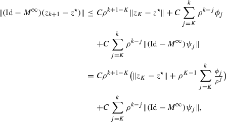  (44)

  By assumption, $\phi _j= C'\eta ^j$, for some constant $C' \ge 0$ and $\eta <\rho$, and we have

  

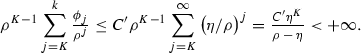
  Setting $C^{''}=C( {||} z_{K}-{z}^\star {||} + \frac{ C' \eta ^{K} }{ \rho - {\eta }}) < +\infty$, we obtain

  $$\begin{aligned} {||} (\mathrm {Id}-M^\infty )({z}_{k+1}-{z}^\star ) {||}&\le C^{''} {\rho }^{k+1-K} + C \sum _{j=K}^{k} {\rho }^{k-j} {||} (\mathrm {Id}-M^\infty )\psi _{j} {||} . \end{aligned}$$

  This, together with the fact that ${||} (\mathrm {Id}-M^\infty )\psi _j {||} = o({||} (\mathrm {Id}-M^\infty )(z_j-{z}^\star ) {||})$ yields the claimed result.

• (iii) From Corollary 6.1(2), we have

  $$\begin{aligned} {z}_{k}- {z}^\star = (M_{\lambda }-M^\infty )^{k+1-K}(z_{K} - {z}^\star ) . \end{aligned}$$

  Moreover, by virtue of Lemma 6.2(iii), $M_\lambda$ is normal and converges linearly to

  $$\begin{aligned} M^\infty =\mathrm {P}_{\left( {T_{x^{\star }}^{J}} \cap T_{x^{\star }}^G\right) \oplus \left( S_{x^{\star }}^J \cap S_{x^{\star }}^G\right) } \end{aligned}$$

  at the optimal rate

  $$\begin{aligned} \rho = {||} M_\lambda - M^\infty {||} = \sqrt{(1-\lambda )^2+\lambda (2-\lambda )\cos ^2\left( \theta _F\left( {T_{x^{\star }}^{J}},T_{x^{\star }}^G\right) \right) }. \end{aligned}$$

  Combining all this then entails

  $$\begin{aligned} \begin{aligned} {||} {z}_{k+1}- {z}^\star {||} \le {||} (M_{\lambda }-M^\infty )^{k+1-K} {||}(z_{K} - {z}^\star )&= {||} M_{\lambda }-M^\infty {||}^{k+1-K}{||} z_{K} - {z}^\star {||} \\&= \rho ^{k+1-K} {||} z_{K} - {z}^\star {||} , \end{aligned} \end{aligned}$$

  which concludes the proof. $\square$

References

Douglas, J., Rachford, H.H.: On the numerical solution of heat conduction problems in two and three space variables. Trans. Am. Math. Soc. 82(2), 421–439 (1956)
Lions, P.L., Mercier, B.: Splitting algorithms for the sum of two nonlinear operators. SIAM J. Numer. Anal. 16(6), 964–979 (1979)
Liang, J., Fadili, M.J., Peyré, G.: Convergence rates with inexact non-expansive operators. Math Program (2015). doi:10.1007/s10107-015-0964-4
Davis, D., Yin, W.: Convergence rate analysis of several splitting schemes. Technical Report arXiv:1406.4834 (2014a)
Davis, D., Yin, W.: Convergence rates of relaxed Peaceman–Rachford and ADMM under regularity assumptions. Technical Report arXiv:1407.5210 (2014b)
Giselsson, P., Boyd, S.: Metric selection in Douglas–Rachford Splitting and ADMM. arXiv preprint arXiv:1410.8479 (2014)
Gabay, D.: Applications of the method of multipliers to variational inequalities. In: Fortin, M., Glowinski, R. (eds.) Augmented Lagrangian Methods: Applications to the Solution of Boundary-Value Problems, pp. 299–331. Elsevier, North-Holland, Amsterdam (1983)
Eckstein, J., Bertsekas, D.P.: On the Douglas–Rachford splitting method and the proximal point algorithm for maximal monotone operators. Math. Program. 55(1–3), 293–318 (1992)
Lewis, A.S.: Active sets, nonsmoothness, and sensitivity. SIAM J. Optim. 13(3), 702–725 (2003)
Demanet, L., Zhang, X.: Eventual linear convergence of the Douglas–Rachford iteration for basis pursuit. Math. Comput. 85(297), 209–238 (2016)
Boley, D.: Local linear convergence of the alternating direction method of multipliers on quadratic or linear programs. SIAM J. Optim. 23(4), 2183–2207 (2013)
Bauschke, H., Cruz, J., Nghia, T., Phan, H., Wang, X.: The rate of linear convergence of the Douglas-Rachford algorithm for subspaces is the cosine of the Friedrichs angle. J. Approx. Theory 185, 63–79 (2014)
Liang, J., Fadili, M.J., Peyré, G., Luke, R.: Activity identification and local linear convergence of Douglas–Rachford/ADMM under partial smoothness. In: Scale Space and Variational Methods in Computer Vision, pp. 642–653. Springer (2015)
Borwein, J.M., Sims, B.: The Douglas-Rachford algorithm in the absence of convexity. In: Bauschke, H.H., Burachik, R.S., Combettes, P.L., Elser, V., Luke, D.R., Wolkowicz, H. (eds.) Fixed-Point Algorithms for Inverse Problems in Science and Engineering, Springer Optimization and Its Applications, vol. 49, pp. 93–109. Springer, New York (2011)
Lewis, A.S., Luke, D.R., Malick, J.: Local linear convergence for alternating and averaged nonconvex projections. Found. Comput. Math. 9(4), 485–513 (2009)
Hesse, R., Luke, D.R., Neumann, P.: Projection methods for sparse affine feasibility: results and counterexamples. Technical Report (2013)
Hesse, R., Luke, D.R.: Nonconvex notions of regularity and convergence of fundamental algorithms for feasibility problems. SIAM J. Optim. 23(4), 2397–2419 (2013)
Phan, H.M.: Linear convergence of the Douglas–Rachford method for two closed sets. Optimization 65(2), 369–385 (2016)
Bauschke, H.H., Dao, M.N., Noll, D., Phan, H.M.: On Slater’s condition and finite convergence of the Douglas–Rachford algorithm for solving convex feasibility problems in Euclidean spaces. J. Global Optim. pp. 1–21 (2015) (In press)
Bauschke, H.H., Combettes, P.L.: Convex Analysis and Monotone Operator Theory in Hilbert Spaces. Springer, Berlin (2011)
Combettes, P.L., Yamada, I.: Compositions and convex combinations of averaged nonexpansive operators. J. Math. Anal. Appl. 425(1), 55–70 (2015)
Bauschke, H.H., Bello Cruz, J.Y., Nghia, T.T.A., Pha, H.M., Wang, X.: Optimal rates of linear convergence of relaxed alternating projections and generalized Douglas-Rachford methods for two subspaces. Numer. Algorithms 73(1), 33–76 (2016). doi:10.1007/s11075-015-0085-4
Combettes, P.L.: Fejér monotonicity in convex optimization. In: Floudas, A.C., Pardalos, M.P. (eds.) Encyclopedia of Optimization, pp. 1016–1024. Springer, Boston (2001). doi:10.1007/978-0-387-74759-0_179
Combettes, P.L.: Solving monotone inclusions via compositions of nonexpansive averaged operators. Optimization 53(5–6), 475–504 (2004)
Bauschke, H.H., Moursi, W.: On the order of the operators in the Douglas–Rachford algorithm. Optim. Lett. (2016). In press (arXiv:1505.02796v1)
Combettes, P.L.: Quasi–Fejérian analysis of some optimization algorithms. Stud. Comput Math 8, 115–152 (2001)
Wright, S.J.: Identifiable surfaces in constrained optimization. SIAM J. Control Optim. 31(4), 1063–1079 (1993)
Lemaréchal, C., Oustry, F., Sagastizábal, C.: The U-lagrangian of a convex function. Trans. Am. Math. Soc. 352(2), 711–729 (2000)
Daniilidis, A., Drusvyatskiy, D., Lewis, A.S.: Orthogonal invariance and identifiability. SIAM J. Matrix Anal. Appl. 35, 580–598 (2014)
Liang, J., Fadili, M.J., Peyré, G.: Activity identification and local linear convergence of Forward–Backward-type methods (2015). Submitted (arXiv:1503.03703)
Hare, W., Lewis, A.S.: Identifying active manifolds. Algorithm. Oper. Res. 2(2), 75–82 (2007)
Rockafellar, R.T., Wets, R.: Variational Analysis, vol. 317. Springer, Berlin (1998)
Rockafellar, R.T.: Convex Analysis, vol. 28. Princeton University Press, Princeton (1997)
Kim, N., Luc, D.: Normal cones to a polyhedral convex set and generating efficient faces in multiobjective linear programming. Acta Math. Vietnam. 25, 101–124 (2000)
Rockafellar, R.T.: Monotone operators and the proximal point algorithm. SIAM J. Control Optim. 14(5), 877–898 (1976)
Luque, F.: Asymptotic convergence analysis of the proximal point algorithm. SIAM J. Control Optim. 22, 277–293 (1984)
Combettes, P.L., Pesquet, J.C.: A proximal decomposition method for solving convex variational inverse problems. Inverse Probl. 24(6), 065,014 (2008). http://stacks.iop.org/0266-5611/24/i=6/a=065014
Raguet, H., Fadili, M.J., Peyré, G.: A generalized forward–backward splitting. SIAM J. Imaging Sci. 6(3), 1199–1226 (2013)
Vaiter, S., Deledalle, C., Fadili, J.M., Peyré, G., Dossal, C.: The degrees of freedom of partly smooth regularizers. Ann. Inst. Stat. Math. (2015) arXiv:1404.5557. To appear
Vaiter, S., Peyré, G., Fadili, M.J.: Model consistency of partly smooth regularizers. Technical Report arXiv:1307.2342, submitted (2015)
Brézis, H.: Opérateurs maximaux monotones et semi-groupes de contractions dans les espaces de Hilbert. In: North-Holland Mathematics Studies. Elsevier, New York (1973)
Hare, W.L., Lewis, A.S.: Identifying active constraints via partial smoothness and prox-regularity. J. Convex Anal. 11(2), 251–266 (2004)
Chavel, I.: Riemannian Geometry: A Modern Introduction, vol. 98. Cambridge University Press, Cambridge (2006)
Miller, S.A., Malick, J.: Newton methods for nonsmooth convex minimization: connections among-Lagrangian, Riemannian Newton and SQP methods. Math. Program. 104(2–3), 609–633 (2005)
Absil, P.A., Mahony, R., Trumpf, J.: An extrinsic look at the Riemannian Hessian. In: Geometric Science of Information, pp. 361–368. Springer (2013)
Lee, J.M.: Smooth Manifolds. Springer, Berlin (2003)
Liang, J., Fadili, M.J., Peyré, G.: Local linear convergence of forward–backward under partial smoothness. In: Advances in Neural Information Processing Systems, pp. 1970–1978 (2014)
Acknowledgements
This work has been partly supported by the European Research Council (ERC project SIGMA-Vision). JF was partly supported by Institut Universitaire de France. The authors would like to thank Russell Luke for helpful discussions.
Author information
Authors and Affiliations
Corresponding author
Additional information
Communicated by Hedy Attouch.