Formal verification of neural agents in non-deterministic environments

Abstract

We introduce a model for agent-environment systems where the agents are implemented via feed-forward ReLU neural networks and the environment is non-deterministic. We study the verification problem of such systems against CTL properties. We show that verifying these systems against reachability properties is undecidable. We introduce a bounded fragment of CTL, show its usefulness in identifying shallow bugs in the system, and prove that the verification problem against specifications in bounded CTL is in coNExpTime and PSpace-hard. We introduce sequential and parallel algorithms for MILP-based verification of agent-environment systems, present an implementation, and report the experimental results obtained against a variant of the VerticalCAS use-case and the frozen lake scenario.

1 Introduction

Forthcoming autonomous and robotic systems, including autonomous vehicles, are expected to use machine learning (ML) methods for some of their components. Differently from more conventional AI systems that are programmed directly by engineers, components based on ML are synthesised from data and implemented via neural networks. In an autonomous system these components could execute functions such as perception [38, 48] and control [30, 33]. Employing ML components has considerable attractions in terms of performance (e.g., image classifiers), and, sometimes, ease of realisation (e.g., non-linear controllers). However, it also raises concerns in terms of overall system safety. Indeed, it is known that neural networks, as presently used, are fragile and hard to understand [52].

If ML components are to be used in safety-critical systems, including various forthcoming autonomous systems, it is essential that they are verified and validated before deployment; standard practice for conventional software. In some areas of AI, notably multi-agent systems (MAS), considerable research has already addressed the automatic verification of AI systems. These concern the validation of either MAS models [20, 35, 41], or MAS programs [8, 14] against expressive AI-inspired specifications, such as those expressible in epistemic and strategy logic. However, with the exceptions discussed below, there is little work addressing the verification of AI systems synthesised from data and implemented via neural networks. This paper makes a contribution in this direction.

Specifically, we formalise and analyse a closed-loop system composed of a reactive neural agent, synthesised from data and implemented by a feed-forward ReLU-activated neural network (ReLU-FFNN), interacting with a non-deterministic environment. Intuitively, the system follows the usual agent-environment loop of observations (of the environment by the agent) and actions (by the agent onto the environment). To model the complexity and partial observability of rich environments, we assume that the neural agent is interacting with a non-deterministic environment, where non-deterministic updates of the environment’s state disallow the agent from fully controlling and fully observing the environment’s state. Under these assumptions, differently from all related work, the system’s evolution is not linear but branching in the future.

We study the verification problem of these systems against a branching time temporal logic. As is known, scalability is a concern in verification and is also an issue in the case of neural systems. To alleviate these difficulties, we are here concerned with a method that is aimed at finding shallow bugs in the system execution, i.e., malfunctions that are realised within a few steps from the system’s initialisation. This kind of analysis has been shown to be of particular importance in applications, see, e.g., bounded model checking (BMC) [12], as, experimentally, bugs are often realised after a limited number of steps. Given this, we focus on a bounded version of CTL, i.e., a language expressing temporal properties realisable in a limited number of execution steps. This allows us to reason about applications where the agents ought to bring about a state of affairs within a finite number of steps, or to verify whether a system remains within safety bounds within a number of steps. This enables us to retain decidability even if we consider infinite domains over the reals for the system’s state variables, whereas the verification problem for plain CTL is undecidable, as we show. To further alleviate the difficulty of the verification problem, we also introduce a novel algorithm that checks for the occurrence of bugs in parallel over the execution paths. As we show, in the case of bounded safety specifications, this enables us to return a bug to the user as soon as a violation is identified on any of the branching paths that are explored in parallel. This gives considerable advantages in applications, as we show in an avionics application.

A key feature of the parallel verification procedure that we introduce lies in its completeness: we can determine with precision when a potentially infinite set of states (up to a number of steps from the system’s initialisation) satisfies a temporal formula. While this results in a heavier computational cost than some incomplete approaches, there are obvious benefits in precise verification, notably the lack of false positives and false negatives. To the best of our knowledge this is the first sound and complete verification framework for closed-loop neural systems that accounts for non-deterministic, branching temporal evolutions.

The rest of the paper is organised as follows. After discussing related work, in Sect. 4 we formally define systems composed by a neural agent, implemented by a ReLU-FFNN, interacting with non-deterministic environments. We analyse the resulting models built on branching executions and define a bounded version of the branching temporal logic CTL to express specifications of these systems. After defining the verification problem, Sect. 5 introduces monolithic and compositional verification algorithms with a complexity study. In this context we show results ranging from undecidability for unbounded reachability, to coNExpTime upper bound for bounded CTL. We present a toolkit for the practical verification of these systems in Sect. 7, implementing said procedure, providing additional functionalities, and reporting the experimental results obtained. We conclude in Sect. 8.

2 Related work

In [3] a closed-loop neural agent-environment system was put forward and analysed. Like the present contribution the agent was modelled via a ReLU-FFNN. However, differently from here, a simple deterministic environment was considered. As a consequence, the system executions were linear and only bounded reachability properties were analysed. [2] extended this work to neural agents formalised via recurrent ReLU-activated neural networks and verified the resulting linear system executions against bounded LTL properties. In contrast, the model put forward here can account for complex, partially observable environments resulting in branching traces, and the strictly more expressive specification language allows for existential and universal quantification over paths. In addition, while the papers above focus on sequential verification procedures, we here develop a parallel approach specifically tailored at identifying shallow bugs efficiently. This requires novel verification algorithms and mixed-integer linear programming [56] (MILP) encodings.

A number of other proposals have also addressed the issue of closed loop systems. For example, [31] presents an approach based on hybrid systems to analyse a control-plant where neural networks are synthesised controllers. Their approach is incomparable with the one here pursued, since they target sigmoidal activation functions (while we focus on ReLU activation functions). Also their verification procedure is not complete, while completeness is a key objective here. Similarly, [15, 28, 32, 57] present work addressing closed loop systems with learned controllers and focus on reachable set estimation and, hence, incomplete techniques for such systems.

Lastly, there has been recent activity on complete approaches for verifying standalone ReLU-FFNNs [6, 9,10,11, 17, 26, 27, 34, 36, 37, 40, 44, 53]. The systems considered in these approaches are not closed-loop and do not incorporate the environment. This makes the problems considered there different from those analysed here; for instance no temporal evolution can be considered for neural network-controlled agents interacting with an environment. We refer to [24, 29, 39] for surveys on the emerging area of verification of neural networks.

In comparison with [1], we here report several novel optimisations in the tool with a more efficient encoding of the discussed aircraft collision avoidance scenario. We also evaluate our tool on an additional reinforcement learning scenario.

More broadly, this line of work is related to long standing efforts in bounded model checking  [7, 47] that are tailored to finding malfunctions easily accessible from the initial states. While our approach is technically different from BMC, it shares with it the characteristic of being more efficient than full exploration methods when only a fraction of the model needs to be explored.

3 Background

In this section we summarise basic concepts pertaining to feed-forward ReLU networks and the formalisation of their verification problem in mixed integer linear programming.

3.1 Feed-forward ReLU networks

A feed-forward neural network (FFNN) [25] is a vector-valued function $\textsf{f} :{\mathbb{R}}^{s_0} \rightarrow {\mathbb{R}}^{s_L}$ that composes a sequence of $L \ge 1$ layers, $\textsf{f}^{1} :{\mathbb{R}}^{s_0} \rightarrow {\mathbb{R}}^{s_1}, \ldots , \textsf{f}^{L} :{\mathbb{R}}^{s_{L-1}} \rightarrow {\mathbb{R}}^{s_L}$. Each layer $\textsf{f}^{i}$, $i \in \left\{ 1,\ldots L \right\}$, composes an affine transformation and an activation function. Formally, we have for $1 \le i \le L$

$$\begin{aligned}&\textsf{f}^{i}(\textsf{x}^{i-1}) \triangleq \textsf{x}^{i}, \\&\quad \textsf{x}^{i} \triangleq \textsf{act}^{i}(\textsf{z}^{i}), \\&\quad \textsf{z}^{i} \triangleq \textsf{W}^{i}\textsf{x}^{i-1} + \textsf{b}^{i}, \end{aligned}$$

where:

• $\textsf{x}^{0}$ is the input to the network and $\textsf{x}^{i}$ is the output of the i-th layer.

• $\textsf{z}^{i}$ is the result of the affine transformation of the i-th layer, known as the pre-activation of the layer, for a weight matrix $\textsf{W}^{i}\in {\mathbb{R}}^{s_i \times s_{i-1}}$ and a bias vector $\textsf{b}^{i}\in {\mathbb{R}}^{s_i}$.

• $\textsf{act}^{i}$ is the activation function of the i-th layer.

Figure 1 gives a graphical representation of a FFNN. Each layer $\textsf{f}^{i}$, $i \in \left\{ 1,\ldots ,L-1 \right\}$, is said to be a hidden layer; the last layer $\textsf{f}^{L}$ of the network is said to be the output layer. Each element of each layer $\textsf{f}^{i}$ is said to be a node (see Fig. 2). The weights and biases of the layers are determined during a training phase which aims at fitting $\textsf{f}$ to a data set consisting of input-output pairs specifying how the network should behave (see, e.g., [21]) for more details).

Here we are only concerned with FFNNs whose hidden layers use the Rectified Linear Unit (ReLU) and the output layer uses the identity function as activation functions; we abbreviate these networks by ReLU-FFNN. The ReLU activation function is widely used in supervised learning tasks because of its effectiveness in training [43]. The function is defined as

$$\begin{aligned} \text{ReLU} (z) \triangleq \max (0,z), \end{aligned}$$

and is applied element-wise to a pre-activation vector $\textsf{z}^{i}$ (see Fig. 3). Since the function consists of two linear parts (0, for $z<0$ and z for $z\ge 0$), it is a piecewise-linear (PWL) function; that is, a function whose input domain can be split into a collection of subdomains on each of which it is an affine function. Consequently, since a ReLU-FFNN composes affine transformations with PWL activation functions, ReLU-FFNNs are also PWL functions.

Fig. 1

A feed-forward neural network of 4 input nodes, 3 hidden layers of 6 nodes each and 4 output nodes

Fig. 2

A node in a feed-forward neural network

Fig. 3

The ReLU activation function

In this paper we are concerned with the reachability problem for ReLU-FFNN. The problem is to establish whether there is an admissible input within a possibly uncountable set of inputs for which a given ReLU-FFNN computes an output within a given set of outputs (see e.g., [4, 5, 16, 34])). Formally, we have

Definition 1

(ReLU-FFNN reachability problem) Given a ReLU-FFNN $\textsf{f}:{\mathbb{R}}^{s_0} \rightarrow {\mathbb{R}}^{s_k}$, a set of inputs ${\mathscr{X}} \subset {\mathbb{R}}^{s_0}$ and a set of outputs ${\mathscr{Y}} \subset {\mathbb{R}}^{s_k}$, the neural network reachability problem is to determine whether

$$\begin{aligned} \text{there exists } \textsf{x} \in {\mathscr{X}} \text{ such that } \textsf{f}(\textsf{x}) \in {\mathscr{Y}}. \end{aligned}$$

The neural network reachability problem is known to be NP-complete [34].

3.2 Mixed integer linear programming

A mixed integer linear programming (MILP) is an optimisation problem whereby a linear objective function over real- and integer-valued variables is sought to be minimised subject to a set of linear constraints. Formally, we have

$$\begin{aligned} \min _{\textsf{x},\textsf{y}} \qquad&c^T \textsf{x} + d^T \textsf{y} \\ \textit{subject} \; to \quad&A \textsf{x} + B \textsf{y} \ge b \\&(\textsf{x}, \textsf{y}) \in {\mathbb{R}}^n \times {\mathbb{Z}}^p, \end{aligned}$$

where $c \in {\mathbb{R}}^n$, $d \in {\mathbb{R}}^p$, $A \in {\mathbb{R}}^{m \times n}$, $B \in {\mathbb{R}}^{m \times p}$ and $b \in {\mathbb{R}}^m$.

For the purposes of this paper, we are interested in the MILP feasibility problem. This is concerned with checking whether a set of MILP constraints is feasible, i.e., whether there exists an assignment to the variables that satisfies all constraints. Therefore, we hereafter assume that the objective function is constant (i.e., it does not depend on the variables), and associate a MILP with a set of linear and typing constraints. It is known that the feasibility problem of MILP is NP-complete [46].

A PWL function can be MILP-encoded using the “Big-M” method. For instance, the pairs (z, x), where $x = \text{ReLU} (z)$ and $z \in [l, u]$ can be found as solutions to the following set of MILP constraints that use a binary variable $\delta$, real-valued variables z and x and constants l and u:

$$\begin{aligned} x \ge 0, \quad x \ge z, \quad x \le u \cdot \delta , \quad x \le z - l \cdot (1-\delta ). \end{aligned}$$

Here, when $\delta = 1$, the constraints imply that $x=z$ and $z\ge 0$, and when $\delta = 0$, the constraints imply that $x=0$ and $z \le 0$. This approach of “switching off” constraints using large enough constants (l and u in this case) is called the “Big-M” method [22]. Equivalently to this formulation, we can compute the same solutions by making use of indicator constraints. These have the form $(\delta =v) \Rightarrow c$, for a binary variable $\delta$, binary value $v \in \left\{ 0,1 \right\}$ and a linear constraint c:

$$\begin{aligned} & (\delta =1) \Rightarrow z \ge 0,\quad (\delta =0) \Rightarrow z \le 0,\\ &(\delta =1) \Rightarrow x = z,\quad (\delta =0) \Rightarrow x = 0. \end{aligned}$$

The indicator constraints are read as follows: if $\delta = 1$ then $z\ge 0$ and $x=z$ should hold, and if $\delta =0$ then $z\le 0$ and $x=0$ should hold. Indicator constraints are supported by all major commercial MILP solvers and can be seen as syntactic sugar for Big-M constraints, where one does not have to provide the big M constant in advance. In particular, indicator constraints can be used to naturally express disjunctive cases, cf. monolithic encoding in Sect. 5.

Since ReLU-FFNNs are PWL, the ReLU-FFNN reachability problem has an exact MILP representation: a feasible solution of the corresponding MILP can be used to find an input $\textsf{x}^{0}$ from the given set of inputs ${\mathscr{X}}$ so that $\textsf{f}(\textsf{x}^{0})$ belongs to the given set of outputs ${\mathscr{Y}}$ [4, 5, 9, 40, 53]. To define the associated MILP, we assume the following: (i) ${\mathscr{X}}$ and ${\mathscr{Y}}$ can be respectively expressed as sets of linear constraints over variables of the inputs and outputs of the network; (ii) a lower bound $\textsf{l}^{i}_{j}$ and an upper bound $\textsf{u}^{i}_{j}$ for each pre-activation $\textsf{z}^{i}_j$ have been computed (the bounds can be computed from ${\mathscr{X}}$ via bound propagation methods, see, e.g., [50, 55]).

Definition 2

(MILP formulation) The MILP formulation of the ReLU-FFNN reachability problem for a ReLU-FFNN $\textsf{f}$, an input set ${\mathscr{X}}$ and an output set ${\mathscr{Y}}$ is

$$\begin{aligned}&\textsf{x}^{0} \in {\mathscr{X}}&\text{(input)}\\&\textsf{z}^{i} = \textsf{W}^{i} \textsf{x}^{i-1} + \textsf{b}^{i}&\text{(pre-activation)} \\&\textsf{x}^{i}_j \ge 0&\text{(ReLU)}\\&\textsf{x}^{i}_j \ge \textsf{z}^{i}_j&\text{(ReLU)}\\&\textsf{x}^{i}_j \le \textsf{u}^{i}_{j} \cdot \delta ^{i}_{j}&\text{(ReLU)} \\&\textsf{x}^{i}_j \le \textsf{z}^{i}_j - \textsf{l}^{i}_{j} \cdot (1 - \delta ^{i}_{j})&\text{(ReLU)} \\&\delta ^{i}_{j} \in \left\{ 0,1 \right\} \qquad \quad 1 \le i < L,\; 1 \le j \le s_i&\text{(ReLU)} \\&\textsf{x}^{L} = \textsf{W}^{L} \textsf{x}^{L-1} + \textsf{b}^{L}&\text{(output)} \\&\textsf{x}^{L} \in {\mathscr{Y}}&\text{(output)} \end{aligned}$$

There exists an input $\textsf{x}^{0} \in {\mathscr{X}}$ such that $\textsf{f}(\textsf{x}^{0}) \in {\mathscr{Y}}$ iff the MILP above is feasible.

4 Neural agent-environment systems

In this section we introduce systems with a neural agent operating on a non-deterministic environment (NANES ). These are an extension to non-deterministic environments of the deterministic neural agent-environment systems put forward in [3].

In contrast to traditional models of agency, where the agent’s behaviour is given in an agent-based programming language, a NANES accounts for the recent shift to synthesise the agents’ behaviour from data [33]; we consider agent protocol functions implemented via ReLU-FFNNs [25]. Differently from [3], following the dynamism and unpredictability of the environments where autonomous agents are typically deployed [42], a NANES models interactions of an agent with a partially observable environment. In this setting an agent cannot observe the full environment state, and therefore cannot deterministically predict the effect of any of its actions.

We now proceed to give a formal description of NANES components: a neural agent and a non-deterministic environment. The description closely follows the formalism of interpreted systems, a mainstream semantics for multi-agent systems [19]. To this end, we fix a set $\textit{S}\subseteq {\mathbb{R}}^m$ of environment states and a set $\textit{Act}\subseteq {\mathbb{R}}^n$ of actions, for $m, n \in {\mathbb{N}}$. We assume that the agent is stateless and that its protocol (also known as action policy) has already been synthesised, e.g., via reinforcement learning [51], and is implemented via a ReLU-FFNN or via a PWL combination of them.

Definition 3

(Neural Agents) Let $\textit{S}$ be a set of environment states.

A neural agent (or simply an agent) $\textit{Ag}$ acting on an environment is defined as the tuple $\textit{Ag}= (\textit{Act},\textit{prot})$, where:

• $\textit{Act}$ is a set of actions;

• $\textit{prot}: S \rightarrow \textit{Act}$ is a protocol function that determines the action the agent will perform given the current state of the environment. Specifically, given ReLU-FFNNs $\textsf{f}_1,\dots ,\textsf{f}_h$, $h \ge 1$, $\textit{prot}$ is a PWL combination of the latter.

When $h=1$, $\textit{prot}(s)$ can be defined, e.g., as $\textsf{f}_{1}(s)$ for $s\in S$.

The environment is stateful and non-deterministically updates its state in response to the actions of the agent.

Definition 4

(Non-deterministic Environments) An environment is a tuple $\textit{E}= (\textit{S}, t_\textit{E})$, where:

• $\textit{S}\subseteq {\mathbb{R}}^m$ is a set of states.

• $t_\textit{E}: \textit{S}\times \textit{Act}\rightarrow 2^\textit{S}$ is a transition function that determines the temporal evolution of the state of the environment. Specifically, given the current state of the environment and the current action of the agent, the transition function returns the set of next possible environment states.

Given the above we can now define a closed-loop system comprising of an agent interacting with an environment.

Definition 5

(NANES ) A Neural Agent operating on a Non-Deterministic Environment System (NANES) is a tuple ${\mathscr{S}}{}= (\textit{Ag}, \textit{E}, I)$ where $\textit{Ag}= (\textit{Act},\textit{prot})$ is a neural agent, $\textit{E}= (\textit{S},t_\textit{E})$ is an environment, and $I\subseteq \textit{S}$ is a closed set¹ of initial states for the environment.

Hereafter we assume the environment’s transition function is PWL and its set of initial states is expressible as a set of linear constraints over integer and real-valued variables. Also, to enable its finite MILP representation, we assume that the function’s branching factor is bounded, i.e., there is a (arbitrarily large) $b\in {\mathbb{N}}$ such that the cardinality of $t_\textit{E}(s,a)$ is bounded by b for all $s\in \textit{S}$ and $a \in \textit{Act}$.

Example 1

Consider as a running example a variant of the FrozenLake scenario [45], where an agent navigates in a grid world consisting of walkable tiles (frozen surface) and non-walkable ones (holes in the ice) leading to the agent falling into water. The goal of the agent is to reach the goal tile while avoiding the holes. At each step the agent chooses a direction to walk, but since walkable tiles are slippery, the resulting movement direction is uncertain and does not only depend on the agent’s choice. Namely, the agent may result moving in any of the three directions: the chosen one and to ones to its left or right, see Fig. 4 for an illustration. We now formalise this scenario as follows.

The agent is defined as $\textit{Ag}_{{\textsf{f}}{\textsf{l}}} = (\textit{Act}_{{\textsf{f}}{\textsf{l}}}, \textit{prot}_{{\textsf{f}}{\textsf{l}}})$, where

• $\textit{Act}_{{\textsf{f}}{\textsf{l}}} = \{{\textsf{d}}_1, {\textsf{d}}_2, {\textsf{d}}_3, {\textsf{d}}_4\} \subseteq {\mathbb{R}}^4$ encodes the directions left (${\textsf{d}}_1$), down (${\textsf{d}}_2$), right (${\textsf{d}}_3$) and up (${\textsf{d}}_4$), where ${\textsf{d}}_i$ is the vector with 1 at i-th position and 0 everywhere else, and

• $\textit{prot}_{{\textsf{f}}{\textsf{l}}}$ is the protocol function implemented via a FFNN network.

The non-deterministic environment models the slippery nature of ice. Here we assume a $3\times 3$ grid world, so formalise the environment as $\textit{E}_{{\textsf{f}}{\textsf{l}}} = (\textit{S}_{{\textsf{f}}{\textsf{l}}}, t_{\textit{E}_{{\textsf{f}}{\textsf{l}}}} )$, where:

• $\textit{S}_{{\textsf{f}}{\textsf{l}}} = \{{\textsf{e}}_1, {\textsf{e}}_2, \ldots , {\textsf{e}}_9\} \subseteq {\mathbb{R}}^9$, where ${\textsf{e}}_i$ is the vector with 1 at i-th position and 0 everywhere else, and

• $t_{\textit{E}_{{\textsf{f}}{\textsf{l}}}} (s, a) = \{\textit{mv}(s, a_{-1}), \textit{mv}(s, a), \textit{mv}(s, a_{+1})\}$,

where $\textit{mv}(s, d)$ returns the state $s'$ resulting from moving from state s in direction d, $a_{-1}$ is the direction to the right of a and $a_{+1}$ is the direction to the left of a when looking in the direction a (e.g., $a_{-1}={\textsf{d}}_1$ and $a_{+1}={\textsf{d}}_3$ for $a={\textsf{d}}_2$). To see that $\textit{mv}(s,d)$ is a PWL function, note that both $\textit{S}$ and $\textit{Act}$ are finite sets.

Finally, we define the set of initial states as $I_{{\textsf{f}}{\textsf{l}}} = \{{\textsf{e}}_1\}$ and the FrozenLake system as ${\mathscr{S}}_{{\textsf{f}}{\textsf{l}}}=(\textit{Ag}_{{\textsf{f}}{\textsf{l}}}, \textit{E}_{{\textsf{f}}{\textsf{l}}}, I_{{\textsf{f}}{\textsf{l}}})$. $\square$

Fig. 4

The FrozenLake surface

With each NANES ${\mathscr{S}}$ we can associate a temporal model ${\mathscr{M}}_{{\mathscr{S}}}$ that is used to interpret temporal specifications.

Definition 6

(Model) Given a NANES system ${\mathscr{S}}{} = (\textit{Ag}, \textit{E}, I)$, its associated temporal model ${\mathscr{M}}_{{\mathscr{S}}}$ is a pair (R, T) where R is the set of environment states reachable from I via T, and $T \subseteq R \times R$ is the successor relation defined by $(s,s') \in T$ iff $s'\in t_E(s,\textit{prot}(s))$.

Fig. 5

The temporal model of the FrozenLake system ${\mathscr{S}}_{\textsf{fl}}$. Each grid depicts the current position of the agent in the environment marked with red colour. Each arrow represents a transition by means of the action labelling the arrow

Example 2

Figure 5 gives a graphical depiction of the temporal model of the FrozenLake system ${\mathscr{S}}_{\textsf{fl}}$, assuming that $\textit{prot}_{\textsf{fl}}({\textsf{e}}_1) = {\textsf{d}}_2$, $\textit{prot}_{\textsf{fl}}({\textsf{e}}_2) = {\textsf{d}}_1$, $\textit{prot}_{\textsf{fl}}({\textsf{e}}_4) = {\textsf{d}}_4$, $\textit{prot}_{\textsf{fl}}({\textsf{e}}_5) = {\textsf{d}}_3$, $\textit{prot}_{\textsf{fl}}({\textsf{e}}_6) = {\textsf{d}}_2$, $\textit{prot}_{\textsf{fl}}({\textsf{e}}_8) = {\textsf{d}}_3$, and $\textit{prot}_{\textsf{fl}}({\textsf{e}}_9) = {\textsf{d}}_2$. $\square$

In the rest of the paper, we assume to have fixed a NANES  ${\mathscr{S}}$ and the associated model ${\mathscr{M}}_{{\mathscr{S}}}$. An ${\mathscr{M}}_{{\mathscr{S}}}$-path, or simply path, is an infinite sequence of states $s_1s_2 \ldots$ where $s_i \in R$ and $s_{i+1}$ is a successor of $s_i$, i.e. $(s_i,s_{i+1}) \in T$, for each $i \ge 1$. Given a path $\rho$ we use $\rho (i)$ to denote the i-th state in $\rho$. For an environment state $s = (c_1,\ldots ,c_m)$, we write $\textsf{paths}(s)$ to denote the set of all paths originating from s and we use s.d to denote its d-th component $c_d$.

We verify NANES against properties expressed in a bounded variant of the temporal logic CTL [13]. It is also possible to verify NANES against bounded versions of LTL, but not pursued here. Inspired by Real-Time Computation Tree Logic (RTCTL) [18], formulae of bounded CTL build upon temporal modalities indexed with natural numbers denoting the temporal depth up to which the formula is evaluated.

Definition 7

(Bounded CTL) Given a set of environment states $S \subseteq {\mathbb{R}}^m$, the bounded CTL specification language over linear inequalities, denoted $\text{bCTL}_{{\mathbb{R}}^<}$, is defined by the following BNF:

$$\begin{aligned} \begin{array}{rcl} \varphi \! \! \! &{} {::}{=} \! \! \! &{} \alpha \big | \varphi \vee \varphi \big | \varphi \wedge \varphi \big | EX^k \varphi \big | AX^k \varphi , \\ \alpha \! \! \! &{} {::}{=} \! \! \! &{} c_1(d_1)+\cdots +c_l(d_l) \gtrless c, \end{array} \end{aligned}$$

where $\gtrless \in \{<,>\}$, $d_i \in \{1,\ldots ,m\}$, $c_i,c \in {\mathbb{R}}$, and $k \in {\mathbb{N}}$.

Here atomic propositions $\alpha$ are linear constraints on the components of a state. For instance, the atomic proposition $(d_1) + (d_2) < 2$ states that “the sum of the $d_1$-st and $d_2$-nd components is less than 2.” The temporal formula $EX^k \varphi$ stands for “there is a path such that $\varphi$ holds after k time steps”, whereas $AX^k \varphi$ stands for “in all paths $\varphi$ holds after k time steps”. Note that the restriction of $\text{bCTL}_{{\mathbb{R}}^<}$ to strict inequalities is crucial to the verification algorithm introduced in the next section; the algorithm relies on encoding the negation of the specification to check into MILP, which does not support strict inequalities.

Example 3

Consider the FrozenLake scenario from Example 1. We are interested in assessing the safety of the scenario in terms of the following specifications:

$$\begin{aligned} \varphi ^k_{\textsf{safe}} = AX^{1}{} \texttt {ha} \wedge \cdots \wedge \ AX^{k} \texttt {ha} \end{aligned}$$

and

$$\begin{aligned} \varphi ^k_{\textsf{succ}} = AX^1\texttt {ha} \wedge \cdots \wedge AX^{k-1}{} \texttt {ha} \wedge AX^k \texttt {goalreached}, \end{aligned}$$

for various values of k, where $\texttt {ha} \triangleq \bigwedge _{h \in \left\{ 3,7 \right\} } (h) < 0.1$ (i.e., holes voided) and $\texttt {goalreached} \triangleq (9) > 0.9$. The formula $\varphi ^k_{\textsf{safe}}$ states that in every evolution of the system the agent always avoids a hole within the first k steps. The formula $\varphi ^k_{\textsf{succ}}$ states that in every evolution of the system the agent always avoids a hole within the first $k-1$ steps and reaches the goal state at the k-th step. Intuitively, the former means that all k-bounded runs are safe (no hole is reached), while the latter means that all k-bounded runs are safe and successful (the goal is reached in the end state). $\square$

We now define the logic $\text{CTL}_{{\mathbb{R}}^<}$ built from the atoms of $\text{bCTL}_{{\mathbb{R}}^<}$.

Definition 8

(CTL) The branching-time logic $\text{CTL}_{{\mathbb{R}}^<}$ is defined by the following BNF:

$$\begin{aligned} \begin{array}{rcl} \varphi \! \! \!&{::}{=} \! \! \!&\alpha \big | \lnot \varphi \mid \varphi \vee \varphi \big | AX \varphi \big | AF\varphi \big | E(\varphi U \varphi ), \end{array} \end{aligned}$$

where $\alpha$ is an atomic proposition in $\text{bCTL}_{{\mathbb{R}}^<}$.

Comparing $\text{bCTL}_{{\mathbb{R}}^<}$ to $\text{CTL}_{{\mathbb{R}}^<}$, we observe that on the one hand $AX^k\varphi$ and $EX^k\varphi$ are expressible, respectively, as $AX (\cdots (AX \varphi )\cdots )$ and $\lnot AX (\cdots (AX \lnot \varphi )\cdots )$, where AX is applied k times. On the other hand, $\text{CTL}_{{\mathbb{R}}^<}$ includes the AF (“in all paths eventually”) and EU (unbounded until) modalities capable of expressing arbitrary reachability, whereas $\text{bCTL}_{{\mathbb{R}}^<}$ admits bounded specifications only. Note that, while $\text{bCTL}_{{\mathbb{R}}^<}$ is clearly less expressive than $\text{CTL}_{{\mathbb{R}}^<}$, it still captures properties of interest. Notably, bounded safety is expressible in $\text{bCTL}_{{\mathbb{R}}^<}$ as $AG^k \textit{safe}$ stating that every state on every path is safe within the first k steps.

We interpret $\text{bCTL}_{{\mathbb{R}}^<}$ formulae on a temporal model as follows.

Definition 9

(Satisfaction)

For a model ${\mathscr{M}}_{{\mathscr{S}}}$, an environment state s, and a $\text{bCTL}_{{\mathbb{R}}^<}$ formula $\varphi$, the satisfaction of $\varphi$ at s in ${\mathscr{M}}_{{\mathscr{S}}}$, denoted $({\mathscr{M}}_{{\mathscr{S}}},s) \models \varphi$, or simply $s\models \varphi$ when ${\mathscr{M}}_{{\mathscr{S}}}$ is clear from the context, is inductively defined as follows:

$$\begin{aligned} \begin{array}{lll} s \models c_1(d_1)+\cdots +c_l(d_l) \gtrless c &{} iff &{} (\sum _{i=1}^lc_i\cdot s.d_i) \gtrless c; \\ s \models \varphi \vee \psi &{} iff &{} s \models \varphi \text{ or }s \models \psi ; \\ s \models \varphi \wedge \psi &{} iff &{} s \models \varphi \text{ and }s \models \psi ; \\ s \models EX^k \varphi &{}\mathrm{iff }&{}\text{ there is }\rho \in \textsf{paths}(s)\text{ such that }\rho (k) \models \varphi ; \\ s \models AX^k \varphi &{}\text{ iff }&{}\text{ for all }\rho \in \textsf{paths}(s)\text{ we have} \rho (k) \models \varphi . \\ \end{array} \end{aligned}$$

We assume the usual definition of satisfaction for $\text{CTL}_{{\mathbb{R}}^<}$; this can be given as standard by using the atomic case from Definition 9.

Although $\text{bCTL}_{{\mathbb{R}}^<}$ does not include negation, it still allows us to express arbitrary CTL formulae of bounded temporal depth since it supports all Boolean and temporal operators with their duals. Useful abbreviations of $\text{bCTL}_{{\mathbb{R}}^<}$ are the temporal modalities $EF^k \varphi$ (“Possibly $\varphi$ within k steps) and $EG^k \varphi$ (“Possibly $\varphi$ for k steps):

$$\begin{aligned}&EF^k \varphi \triangleq EX^1 \varphi \vee \cdots \vee EX^k \varphi \\&EG^k \varphi \triangleq EX^1 \varphi \text{ if } k =1; EX^1 (\varphi \wedge EG^{k-1} \varphi ) \text{ if } k > 1. \end{aligned}$$

The dual temporal modalities $AG^k \varphi$ and $AF^k \varphi$, prefixed by the universal path quantifier, are analogously defined:

$$\begin{aligned}&AG^k \varphi \triangleq AX^1 \varphi \wedge \cdots \wedge AX^k \varphi \\&AF^k \varphi \triangleq AX^1 \varphi \text{ if } k =1; AX^1 (\varphi \vee AF^{k-1} \varphi ) \text{ if } k > 1. \end{aligned}$$

Moreover, bounded until $E(\varphi U^k \psi )$ (“there is a path such that $\psi$ holds within k time steps, and where $\varphi$ holds up until then”) can be defined by the abbreviations

$$\begin{aligned}&E(\varphi U^1 \psi ) \triangleq \psi \vee (\varphi \wedge EX^1 \psi ), \\&E(\varphi U^k \psi ) \triangleq \psi \vee (\varphi \wedge EX^1 E(\varphi U^{k-1} \psi )) \text{ for }k > 1, \end{aligned}$$

and analogously with $A(\varphi U^k \psi )$.

We also note that the formula $QX^k\varphi$, for $Q \in \{A,E\}$, is equivalent to $QX^1 (\cdots (QX^1 \varphi )\cdots )$, where $QX^1$ is applied k times to $\varphi$.

A specification $\varphi$ is said to be satisfied by ${\mathscr{S}}$ if $({\mathscr{M}}_{{\mathscr{S}}},s) \models \varphi$ for all initial states $s \in I$. We denote this by ${\mathscr{S}}\models \varphi$. It follows that, for example, to check bounded safety we need to verify that from all (possibly infinitely many) initial states no state (out of possibly infinitely many) within the first k evolutions is an unsafe state. This is the basis of the verification problem that we define below.

Definition 10

(Verification problem) Given a NANES ${\mathscr{S}}$ and a formula $\varphi$, determine whether ${\mathscr{S}}{} \models \varphi$.

Remark 1

The verification problem is uniquely associated with a model checking problem which is to check whether ${\mathscr{M}}_{{\mathscr{S}}}\models \varphi$ given ${\mathscr{M}}_{{\mathscr{S}}}$ and $\varphi$.

However, when the input is specified in terms of a NANES ${\mathscr{S}}$ and a specification $\varphi$, generally, the size (of the relevant part) of the model ${\mathscr{M}}_{{\mathscr{S}}}$ grows exponentially in the size of the input.

In the next section we study the decidability and complexity of the verification problem here introduced.

5 The verification problem

In this section we study the verification problem for a NANES against CTL and $\text{bCTL}_{{\mathbb{R}}^<}$ specifications. First, we show that verifying against CTL formulae is undecidable for deterministic environments and simple reachability properties. In the rest of the section, we focus on bounded CTL, where we develop a decision procedure for the verification problem based on producing a single MILP and checking its feasibility. Then we devise a parallelisable version of the procedure that produces multiple MILPs and that can be particularly efficient at finding counter-examples for bounded safety properties. Following this, we analyse the computational complexity of the verification problem against $\text{bCTL}_{{\mathbb{R}}^<}$ formulae.

5.1 Unbounded CTL

In this subsection we show undecidability of the verification problem for deterministic NANES against simple reachability properties, where a deterministic NANES is a tuple $(\textit{Ag}=(\textit{Act}, \textit{prot}), E=(S,t_E), I)$, where $|t_E(s,a)| = 1$ for all $s \in S$ and $a \in \textit{Act}$. The undecidability result for arbitrary NANES and full CTL follows.

Theorem 1

Verifying deterministic NANES against formulae of the form $AF \alpha$ is undecidable.

Proof

We show the result by reduction from the Halting problem which is known to be undecidable. Let $M = \langle Q, \varSigma , \varSigma _0, \delta , q_0, q_a\rangle$ be a Turing machine, where

• $Q=\{1,\dots ,k\}$ is a finite set of states,

• $\varSigma =\{0,1,2\}$ is a finite tape alphabet, where we treat 0 as the blank symbol,

• $\varSigma _0=\{1,2\}$ is the set of input symbols,

• $q_0,q_a \in Q$ are the initial and accepting states, respectively, and

• $\delta : (Q\setminus \{q_a\}) \times \varSigma \mapsto Q \times \varSigma \times \{\text{L},\text{R}\}$ is the transition function such that given a state $q \in Q\setminus \{q_a\}$ and a tape symbol $\sigma$, $\delta (q,\sigma )=(q',\sigma ',m)$ for $q' \in Q$, $\sigma '\in \varSigma$ and $m\in \{\text{L},\text{R}\}$ with the following meaning: if the Turing machine is in the state q and currently reads symbol $\sigma$ (i.e., the content of the cell where the head currently is is $\sigma$), then write in the current cell $\sigma '$, move the head left if $m=\text{L}$ and right if $m=\text{R}$, and change the state to $q'$.

We can assume that the tape of M is open-ended only on the right-hand side, that is, the head never goes to the left of the first cell (cell number 1). The Halting problem defined as “given an input string $\omega _0 \subseteq {\varSigma _0}^h$, decide whether M halts on $\omega _0=a_1\dots a_h$, that is, whether M eventually enters $q_a$” for such Turing machine is known to be undecidable.

We construct a NANES ${\mathscr{S}}=((\textit{Act},\textit{prot}), (S,t_E), I)$ and an unbounded temporal formula $\varphi$ such that ${\mathscr{S}}\models \varphi$ iff M halts on $\omega _0=a_1\dots a_h$.

• each state of ${\mathscr{S}}$ encodes the current configuration of the Turing machine, that is, the current state, the content of the tape and position of the head on the tape. We account for the position of the head implicitly by storing the content of the tape to the left and to the right of the head. Therefore, the state space S consists of tuples $g=(q,\omega _l,\sigma ,\omega _r)$ where

  • $q\in Q$,

  • $\omega _l$ represents the left part of the tape and is a real number from [0, 0.3) whose ith digit after the dot stores the content of the ith cell to the left of the head, and hence is one of 0, 1 or 2.

  • $\sigma \in \varSigma$ is the symbol under the head.

  • $\omega _r$ represents the right part of the tape and is a real number from [0, 0.3) whose ith digit after the dot stores the content of the ith cell to the right of the head, and hence is one of 0, 1 or 2.

  The left $\omega _l$ and right $\omega _r$ parts of the tape can be seen as stacks with the symbols in the top part being closer to the head, while in the lower part further from the head. In what follows, we refer to them as left stack and right stack, respectively. Moving the head to the right then corresponds to popping the top symbol from the right stack and pushing $\sigma$ onto the left stack, and the other way around.

• $I = \{(q_0, 0.0, a_1, 0.a_2\dots a_h)\}$

• $\textit{Act} = \{a\}$ for some $a \in {\mathbb{R}}$.

• the agent’s network N computes the constant (hence, linear) function $\textit{prot}(q, \omega _l, \sigma ,\omega _r) = a$.

• the transition function is deterministic and follows closely the transition function $\delta$ of M. The main technicality here is to implement $\delta$ by suitably updating $\omega _l$, $\sigma$ and $\omega _r$. Specifically, $t_E((q,\omega _l,\sigma ,\omega _r), a) = (q',\omega _l',\sigma ',\omega _r')$ where

  • $\sigma _l = \lfloor \omega _l\cdot 10\rfloor$ and $\sigma _r = \lfloor \omega _r\cdot 10\rfloor$ are the top symbols of $\omega _l$ and $\omega _r$, respectively,

  • there exists $\sigma _n$ and m such that $\delta (q,\sigma ) = (q',\sigma _n,m)$,

  • $\omega _l' = (\sigma _n + \omega _l)\cdot 0.1$, $\sigma '=\sigma _r$ and $\omega _r' = \omega _r\cdot 10 -\sigma _r$ if $m=\text{R}$, that is, we push the new symbol $\sigma _n$ to left stack and pop the top symbol from the right stack, and

  • $\omega _l' = \omega _l\cdot 10 -\sigma _l$, $\sigma '=\sigma _l$ and $\omega _r' = (\omega _r + \sigma _n) \cdot 0.1$ if $m=\text{L}$, that is, we pop the top symbol from the left stack and push $\sigma _n$ onto the right stack.

• $\varphi$ is the reachability specification $EF ((1) > |Q|-1)$, where we assume that all states in Q are numbered from 1 to |Q|, and $q_a$ is the state number |Q|.

It is straightforward to see that ${\mathscr{S}}$ and $\varphi$ are as required.

It can also be seen that $t_E$ is a linearly definable function. We only show an implementation of the function computing the integer part $\lfloor x \rfloor$ of a non-negative real number $x \in [0,3)$ via a ReLU FFNN $N_{\lfloor \cdot \rfloor }$. Then $t_E$ can be computed by combining it with appropriate linear expressions and conditional statements.

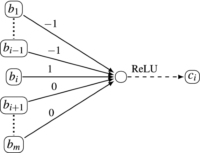
Below we depict the network $N_{\lfloor \cdot \rfloor }$ in which each hidden neuron is split into two nodes, resulting from the linear transformation of the previous layer, and the labelled result of ReLU activation; the weights are drawn on the edges and biases below the nodes. For instance, $y_1$ is computed from x as $\text{ReLU}(3\cdot x - 4)$, while $\lfloor x\rfloor$ is computed from $z_1$ and $z_2$ as $-z_1-z_2+2$.

To see that this network computes what is intended, observe that the intermediate values $y_i$ and $z_i$ are as follows:

• $y_1 > 0$ iff $x \ge 2$

• $z_1 = 0$ if $x \ge 2$, and $z_1 = 1$ if $x < 2$

• $y_2 > 0$ iff $x \ge 1$

• $z_2 = 0$ if $x \ge 1$, and $z_2 = 1$ if $x < 1$

Conversely, we can construct a NANES ${\mathscr{S}}'=((\textit{Act}',\textit{prot}'), (S',t_E'), I')$ where $t_E'$ is a linear function and $\textit{prot}'$ is a PWL function such that ${\mathscr{S}}'\models \varphi$ iff M halts on $\omega _0$. Namely,

• $\textit{Act}' = S' = S$, $I' = I$,

• $t_E'(s,a) = a$, and

• $\textit{prot}'(s) = t_E(s,\_)$.

$\square$

We observe that the above result holds even for strongly restricted NANES where either the protocol or the transition function is linear (but not both at the same time). Intuitively, since every piecewise-linear function can be exactly represented by a ReLU-activated neural network, NANES (even with deterministic environment transition function) are able to simulate recurrent neural networks that are known to be Turing-complete [49].

As a corollary, we obtain undecidability of the verification problem against full CTL.

Corollary 1

Verifying NANES against $\text{CTL}_{{\mathbb{R}}^<}$ formulae is undecidable.

5.2 Bounded CTL

We now proceed to investigate the verification problem for the bounded CTL specification language. We start by showing an auxiliary result that allows us to assume without loss of generality that the cardinality of $t_E(s,a)$ is the same for each state s and action a.

Lemma 1

Given a NANES ${\mathscr{S}}=((\textit{Act},\textit{prot}), (S,t_E), I)$ and specification $\varphi \in \text{bCTL}_{{\mathbb{R}}^<}$, there is a NANES ${\mathscr{S}}' = ((\textit{Act},\textit{prot}'), (S',t_E'), I')$, such that $|t_E'(s_1,a_1)| = |t_E'(s_2,a_2)|$ for all $s_1, s_2 \in S'$, and $a_1, a_2 \in \textit{Act}$, and a specification $\varphi '\in \text{bCTL}_{{\mathbb{R}}^<}$ such that ${\mathscr{S}}\models \varphi$ iff ${\mathscr{S}}' \models \varphi '$.

Proof

Consider $b = \max _{s\in S,a\in \textit{Act}}|t_E(s,a)|$, following the assumption on boundedness of $|t_E(s,a)|$ for all $s\in S$ and $a\in \textit{Act}$. First, we define a NANES ${\mathscr{S}}' = ((\textit{Act},\textit{prot}'), (S',t_E'), I')$ so that $|t_E'(s,a)|=b$ for all $s \in S'$, $a\in \textit{Act}$:

• $S' = S\times \{0,1\}$ and $I'=I \times \{1\}$. The added dimension indicates whether a state is valid (1) or not (0).

• The agent’s protocol function $\textit{prot}'$ is defined as $\textit{prot}'((s,f)) = \textit{prot}(s)$ for each $s\in S$, $f\in \{0,1\}$.

• The transition function $t_E'$ is defined as

  • $t_E'((s,1), a) = t_E(s,a)\times \{1\} \cup \{(s_1,0),\dots ,(s_{b-l},0)\}$,

  • $t_E'((s,0), a) = \{(s_1,0),\dots ,(s_{b},0)\}$

  for $s\in S$, $a\in \textit{Act}$, $|t_E(s,a)| = l$ and $s_1,\dots ,s_{b}$ pairwise distinct states from S.

Now, suppose that $S = {\mathbb{R}}^m$. We set specification $\varphi '$ to be the formula in $\text{bCTL}_{{\mathbb{R}}^<}$ obtained from $\varphi$ by replacing each atomic proposition $\alpha$ with $\alpha \wedge ((m + 1) > 0.9)$. It is straightforward to see that ${\mathscr{S}}\models \varphi$ iff ${\mathscr{S}}'\models \varphi '$, and hence, $\varphi '$ is as required. $\square$

In the rest of this section we assume that $|t_E(s,a)| = b$ for all s and a, and that $t_E$ is given as $b$ piecewise-linear (PWL) functions $t_i:{\mathbb{R}}^{m+n}\rightarrow {\mathbb{R}}^m$. To see that the latter is possible, note that, assuming an ordering (e.g., lexicographical) on the elements of ${\mathbb{R}}^m$, we can define $t_i$ to return the i-th element of the result by $t_E$, which is clearly a PWL function. Also note that this assumption is used when devising the verification procedure presented below.

The procedures that we put forward recast the verification problem to the MILP feasibility problem (see Sect. 3 for preliminaries on MILP). Given a MILP program $\pi$, we use $\textit{vars}(\pi )$ to denote the set of variables in $\pi$. Denote by ${\mathfrak {a}}$ the assignment function ${\mathfrak {a}} : \textit{vars}(\pi ) \rightarrow {\mathbb{R}}$, which defines the specific (binary, integer or real) value assigned to a MILP program variable. We write ${\mathfrak {a}} \models \pi$ if ${\mathfrak {a}}$ satisfies $\pi$, i.e., if ${\mathfrak {a}}(\delta ) \in \{0,1\}$ for each binary variable $\delta$, ${\mathfrak {a}}(\iota ) \in {\mathbb{N}}$ for each integer variable $\iota$, and all constraints in $\pi$ are satisfied. Hereafter, we denote by boldface font tuples $\mathbf {x}$ of MILP variables (of length m for $S \subseteq {\mathbb{R}}^m$ the set of environment states) representing an environment state and call them state variables.

As a stepping stone in our procedures, we encode the computation of a successor environment state as a composition of the protocol function $\textit{prot}$ and of the transition functions $t_i$. By assumption, $\textit{prot}$ and each $t_i$ is a PWL function, and so the predicate $\mathbf {y} = t_i(\mathbf {x}, \textit{prot}(\mathbf {x}))$ is expressible as a set of MILP constraints by means of the Big-M method, which we denote by $C_i(\mathbf {x},\mathbf {y})$ (note that $\mathbf {x}\cup \mathbf {y}\subset \textit{vars}(C_i(\mathbf {x},\mathbf {y}))$). Solutions of $C_i(\mathbf {x},\mathbf {y})$ represent pairs of consecutive environment states:

Lemma 2

Let $C_i(\mathbf {x},\mathbf {y})$ be a MILP program corresponding to $\mathbf {y} = t_i(\mathbf {x}, \textit{prot}(\mathbf {x}))$. Given two states s and $s'$ in ${\mathscr{M}}_{{\mathscr{S}}}$, we have that $s' = t_i(s,\textit{prot}(s))$ iff there is an assignment ${\mathfrak {a}}$ to $\textit{vars}(C_i(\mathbf {x},\mathbf {y}))$ such that $s = {\mathfrak {a}}(\mathbf {x})$, $s'={\mathfrak {a}}(\mathbf {y})$, and ${\mathfrak {a}} \models C_i(\mathbf {x},\mathbf {y})$.

Proof

The result follows from the fact that $t_i(\mathbf {x},\textit{prot}(\mathbf {x}))$ is a PWL function and that every PWL function can be encoded into a set of MILP constraints. Details can be found in [3]. $\square$

Fig. 6

Monolithic encoding $\pi _{{\mathscr{S}}\!\!,\,\varphi }$ for $\varphi \in \text{bCTL}_{{\mathbb{R}}^\le }$, where for a set of constraints $\pi$, $(\delta =v)\Rightarrow \pi$ abbreviates the set of indicator constraints $\{ (\delta =v)\Rightarrow c \big | c\in \pi \}$

5.2.1 Monolithic encoding

First, we devise a recursive encoding of a NANES and a formula into a single MILP, referred to as monolithic encoding, and define the corresponding monolithic verification procedure.

Denote by $\text{bCTL}_{{\mathbb{R}}^\le }$ the bounded CTL language over atomic propositions $\alpha$ where $\gtrless \in \{\le , \ge \}$ (i.e., linear constraints over non-strict inequalities). Given a NANES ${\mathscr{S}}$ and a formula $\varphi \in \text{bCTL}_{{\mathbb{R}}^\le }$, we construct a MILP program $\pi _{{\mathscr{S}}\!\!,\,\varphi }$, whose feasibility corresponds to the existence of a state in ${\mathscr{M}}_{{\mathscr{S}}}$ that satisfies $\varphi$. For ease of presentation, and without loss of generality, we assume that $\varphi$ may contain only the temporal modalities $EX^1$ and $AX^1$, for which we write EX and AX, respectively.

We now define the monolithic encoding $\pi _{{\mathscr{S}}\!\!,\,\varphi }$.

Definition 11

Given a NANES ${\mathscr{S}}$ and a formula $\varphi \in \text{bCTL}_{{\mathbb{R}}^\le }$, their monolithic MILP encoding $\pi _{{\mathscr{S}}\!\!,\,\varphi }$ is defined as the MILP program $\pi _{{\mathscr{S}}\!\!,\,\varphi }(\mathbf {x})$, where $\mathbf {x}$ is a tuple of fresh state variables, and $\pi _{{\mathscr{S}}\!\!,\,\varphi }(\mathbf {x})$ is built inductively using the rules in Fig. 6.

The monolithic encoding creates one single MILP that entirely accounts for the semantics of the formula, and in particular, every kind of disjunction (in $\varphi _1\vee \varphi _2$ and $EX\varphi$) is handled by appropriate MILP constraints. Intuitively, the variables $\mathbf {x}$ in the program $\pi _{{\mathscr{S}}\!\!,\,\varphi }(\mathbf {x})$ refer to the states that satisfy the formula $\varphi$. In Fig. 6, the base case $\pi _{{\mathscr{S}}\!\!,\,\alpha }(\mathbf {x})$ for an atom $\alpha$ produces the MILP program consisting of a single linear constraint corresponding to $\alpha$ and using variables in $\mathbf {x}$. Each inductive case depends on the state variables $\mathbf {x}$ but might in turn generate programs for subformulas which depend on freshly created state variables different to $\mathbf {x}$ (such as $\mathbf {y}$, $\mathbf {y}_1$, $\mathbf {y}_2$, etc). All other auxiliary variables employed in the encoding are also fresh, preventing undesirable interactions between unrelated branches of the program.

• Disjunction uses a binary variable $\delta$ and two sets of indicator constraints. In a feasible assignment ${\mathfrak {a}}$, when $\delta$ is 1, $\varphi _1$ is satisfied and the values of $\mathbf {x}$ are assigned according to $\varphi _1$, while when $\delta$ is 0, $\varphi _2$ holds and the values of $\mathbf {x}$ are assigned as per $\varphi _2$.

• We encode conjunction as the union of the constraints for each of the conjuncts, which all must be satisfied at the same time.

• We encode an operator EX by a $b$-ary disjunction using binary variables $\delta _1,\dots ,\delta _b$. Each of the possible $b$ next states is chosen by activating one of $\delta _i$ hence ensuring that the relevant $C_i(\mathbf {x},\mathbf {y})$ is satisfied. The variables $\mathbf {y}$ refer to the successor state which must satisfy $\varphi$, therefore, the subprogram for $\varphi$ depends on $\mathbf {y}$. Notably, only one copy of $\pi _{{\mathscr{S}}\!\!,\,\varphi }$ is required.

• To satisfy $AX\varphi$, all $b$ possible successor states should satisfy $\varphi$, and so we take the union of all $C_i(\mathbf {x},\mathbf {y}_i)$ and of $b$ copies of $\pi _{{\mathscr{S}}\!\!,\,\varphi }$, each depending on one of the successor state variables $\mathbf {y}_i$.

Note that the size of $\pi _{{\mathscr{S}}\!\!,\,\varphi }$ may grow exponentially due to $b$ repetitions of $\pi _{{\mathscr{S}}\!\!,\,\psi }$ in $\pi _{{\mathscr{S}}\!\!,\,AX\psi }(\mathbf {x})$; for $\varphi = AX^k \alpha$, the size of $\pi _{{\mathscr{S}}\!\!,\,\varphi }$ is $O(k \cdot b^k \cdot |{\mathscr{S}}|)$. The same estimate works in the general case for the temporal bound k of $\varphi$. On the other hand, when $\varphi$ contains no AX operator, the size of $\pi _{{\mathscr{S}}\!\!,\,\varphi }$ remains polynomial $O(k \cdot b\cdot |{\mathscr{S}}|)$.

We can prove that $\pi _{{\mathscr{S}}\!\!,\,\varphi }$ is as intended.

Lemma 3

Given a NANES ${\mathscr{S}}$, a formula $\varphi \in \text{bCTL}_{{\mathbb{R}}^\le }$ and a state s in ${\mathscr{M}}_{{\mathscr{S}}}$, the following are equivalent:

• 1. $s \models \varphi$.

• 2. There exists an assignment ${\mathfrak {a}}$ to $\textit{vars}(\pi _{{\mathscr{S}}\!\!,\,\varphi }(\mathbf {x}))$ such that ${\mathfrak {a}} \models \pi _{{\mathscr{S}}\!\!,\,\varphi }(\mathbf {x})$ and $s = {\mathfrak {a}}(\mathbf {x})$.

Proof

Let s be a state in ${\mathscr{M}}_{{\mathscr{S}}}$. We prove the statement by induction on the structure of $\varphi$. Clearly, the thesis holds when $\varphi$ is an atomic proposition.

Suppose that the thesis holds for $\varphi _1$ and $\varphi _2$. Consider the following cases:

$$\begin{aligned} \varphi= & {} \varphi _1\vee \varphi _2.\text{ Then}\\&s\models \varphi _1\vee \varphi _2 \Leftrightarrow \\&s\models \varphi _1\text{ or }s\models \varphi _2 \Leftrightarrow \end{aligned}$$

there exists ${\mathfrak {a}}_1$ s.t. ${\mathfrak {a}}_1 \models \pi _{{\mathscr{S}}\!\!,\,\varphi _1}(\mathbf {x})$, ${\mathfrak {a}}_1(\delta )=1$ and $s={\mathfrak {a}}_1(\mathbf {x})$, or there exists ${\mathfrak {a}}_2$ s.t. ${\mathfrak {a}}_2 \models \pi _{{\mathscr{S}}\!\!,\,\varphi _2}(\mathbf {x})$, ${\mathfrak {a}}_1(\delta )=0$ and $s={\mathfrak {a}}_2(\mathbf {x})$ $\Leftrightarrow$

there exists ${\mathfrak {a}}$ s.t. ${\mathfrak {a}}\models \pi _{{\mathscr{S}}\!\!,\,\varphi _1\vee \varphi _2}(\mathbf {x})$, and $s = {\mathfrak {a}}(\mathbf {x})$.

$$\begin{aligned} \varphi= & {} \varphi _1\wedge \varphi _2.\text{ Then}\\&s\models \varphi _1\wedge \varphi _2 \Leftrightarrow \\&s\models \varphi _1\text{ and }s\models \varphi _2 \Leftrightarrow \end{aligned}$$

there exists ${\mathfrak {a}}_1$ s.t. ${\mathfrak {a}}_1 \models \pi _{{\mathscr{S}}\!\!,\,\varphi _1}(\mathbf {x})$ and $s={\mathfrak {a}}_1(\mathbf {x})$, and there exists ${\mathfrak {a}}_2$ s.t. ${\mathfrak {a}}_2 \models \pi _{{\mathscr{S}}\!\!,\,\varphi _2}(\mathbf {x})$ and $s={\mathfrak {a}}_2(\mathbf {x})$ $\Leftrightarrow ^{\textit{vars}(\pi _{{\mathscr{S}}\!\!,\,\varphi _1}(\mathbf {x})) \cap \textit{vars}(\pi _{{\mathscr{S}}\!\!,\,\varphi _2}(\mathbf {x})) = \mathbf {x}}$

$$\begin{aligned} {\mathfrak {a}}_1\cup {\mathfrak {a}}_2 \models \pi _{{\mathscr{S}}\!\!,\,\varphi _1}(\mathbf {x}) \cup \pi _{{\mathscr{S}}\!\!,\,\varphi _2}(\mathbf {x}).\end{aligned}$$

$$\begin{aligned} \varphi= & {} EX\varphi _1.\text{ Then}\\&s\models EX\varphi _1 \Leftrightarrow \end{aligned}$$

there exists a successor $s'$ of s in ${\mathscr{M}}_{{\mathscr{S}}}$ s.t. $s'\models \varphi _1$ $\Leftrightarrow$

there exists $i\in \{1,\dots ,k\}$ and an assignment ${\mathfrak {a}}_i$ such that ${\mathfrak {a}}_i(\delta _i)=1$, ${\mathfrak {a}}_i(\delta _j)=0$ for $j\ne i$, ${\mathfrak {a}}_i\models C_i(\mathbf {x},\mathbf {y})$, ${\mathfrak {a}}_i(\mathbf {x})=s$ and ${\mathfrak {a}}_i(\mathbf {y})=s'$, and there exists an assignment ${\mathfrak {a}}'$ s.t. ${\mathfrak {a}}'\models \pi _{{\mathscr{S}}\!\!,\,\varphi _1}(\mathbf {y})$ and ${\mathfrak {a}}'(\mathbf {y})=s'$ $\Leftrightarrow$

there exists ${\mathfrak {a}}$ s.t. ${\mathfrak {a}}\models \pi _{{\mathscr{S}}\!\!,\,EX\varphi _1}(\mathbf {x})\text{ and } {\mathfrak {a}}(\mathbf {x})=s.$

$$\begin{aligned} \varphi= & {} AX\varphi _1.\text{ Then}\\&s\models AX\varphi _1 \Leftrightarrow \end{aligned}$$

for every successor $s_i$ of s in ${\mathscr{M}}_{{\mathscr{S}}}$ it holds that $s_i\models \varphi _1$, $i=1,\dots ,k$, $\Leftrightarrow$

for every successor $s_i$ of s in ${\mathscr{M}}_{{\mathscr{S}}}$ it holds that there exists ${\mathfrak {a}}_i$ s.t. ${\mathfrak {a}}_i\models \pi _{{\mathscr{S}}\!\!,\,\varphi _1}(\mathbf {y}_i)$ and ${\mathfrak {a}}_i(\mathbf {y}_i)=s_i$, $i=1,\dots ,k$, $\Leftrightarrow$

there exists ${\mathfrak {a}}$ s.t. ${\mathfrak {a}}\models \pi _{{\mathscr{S}}\!\!,\,AX\varphi _1}(\mathbf {x})\text{ and } {\mathfrak {a}}(\mathbf {x})=s.$ $\square$

Finally, we are ready to devise a procedure that solves the verification problem by checking feasibility of the monolithic MILP encoding for the negation of the property to be verified together with a restriction to the initial states of ${\mathscr{S}}$, $\pi _{{\mathscr{S}}\!\!,\,\textsf{NNF}(\lnot \varphi ) \wedge \varphi _I}$. The idea here is to look for a proof that the property is not satisfied by a state $s\in I$. A feasible solution to $\pi _{{\mathscr{S}}\!\!,\,\textsf{NNF}(\lnot \varphi )\wedge \varphi _I}$ then provides such a proof in the form of a counter-example. Conversely, infeasibility implies that no counter-example could be found, and so the property is satisfied.

The procedure is given by Algorithm 1. Recall that strict inequalities are not supported in the MILP solver. Note that by our assumption the set I of initial states is closed and expressible as a set of linear constraints. Therefore, we can represent I by a Boolean formula from $\text{bCTL}_{{\mathbb{R}}^\le }$ (i.e., a formula without temporal operators). For instance, the hyper-rectangle $[l_1,u_1]\times \cdots \times [l_m,u_m]$ is represented by the formula

$$\begin{aligned} (1)\ge l_1 \wedge (1)\le u_1 \wedge \cdots \wedge (m)\ge l_m \wedge (m)\le u_m. \end{aligned}$$

Further note that we only pass $\lnot \varphi$ (the negation of the specification) to the encoding in negation normal form (NNF). In this process, negation is eliminated by pushing it down and through the atoms resulting in all strict inequalities of atoms of the original specification $\varphi$ being converted to non-strict inequalities. Therefore, $\varphi '=\textsf{NNF}(\lnot \varphi ) \wedge \varphi _I$ is a formula from $\text{bCTL}_{{\mathbb{R}}^\le }$, so $\pi _{{\mathscr{S}}\!\!,\,\varphi '}$ is well-defined and can be processed by an MILP solver.

Soundness and completeness of the verification procedure relies on Lemma 3 and is shown by the following.

Theorem 2

Given a NANES ${\mathscr{S}}$ and a formula $\varphi \in \text{bCTL}_{{\mathbb{R}}^<}$, Algorithm 1 returns False iff ${\mathscr{S}}\not \models \varphi$.

Proof

Suppose that Algorithm 1 returns False. It follows that $\pi _{{\mathscr{S}}\!\!,\,\lnot \varphi \wedge \varphi _I}(\mathbf {x})$ is feasible, and there exists an assignment ${\mathfrak {a}}$ to $\textit{vars}(\pi _{{\mathscr{S}}\!\!,\,\lnot \varphi \wedge \varphi _I}(\mathbf {x}))$ such that ${\mathfrak {a}}\models \pi _{{\mathscr{S}}\!\!,\,\lnot \varphi \wedge \varphi _I}(\mathbf {x})$. Take $s={\mathfrak {a}}(\mathbf {x})$. Since $\varphi _I$ is a Boolean formula (without temporal operators), it is straightforward to see that $s\in I$. Therefore s is a state in ${\mathscr{M}}_{{\mathscr{S}}}$, and by Lemma 3 we have that $s\models \varphi _I$ and $s\models \lnot \varphi$. It follows that $s\not \models \varphi$, and consequently, ${\mathscr{S}}\not \models \varphi$. Conversely, if there exists $s \in I$ such that $s\not \models \varphi$, we obtain that there is an assignment satisfying $\pi _{{\mathscr{S}}\!\!,\,\lnot \varphi \wedge \varphi _I}(\mathbf {x})$, and therefore Algorithm 1 returns False. $\square$

5.2.2 Compositional encoding

Observe that due to its handling of disjunctions, the previously introduced monolithic encoding $\pi _{{\mathscr{S}}\!\!,\,\varphi }$ might result in excessively large programs whose feasibility is a computationally expensive task. We now propose a different encoding that instead of delegating disjunction to the MILP solver (the $\varphi _1\vee \varphi _2$ and $EX\varphi$ cases) creates a separate program for each disjunct, whose feasibility results can be combined to solve the verification problem. More specifically, for a formula $\varphi$, we define a set $\varPi _{{\mathscr{S}},\varphi }$ of MILP programs with the property that there exists a state s in ${\mathscr{M}}_{{\mathscr{S}}}$ such that $s \models \varphi$ iff at least one of the programs in $\varPi _{{\mathscr{S}},\varphi }$ is feasible.

Below, given a set C of linear constraints, we write [C] to denote the respective MILP program. Given sets $A = \{[A_1],\dots ,[A_p]\}$ and $B = \{[B_1],\dots ,[B_q]\}$ of MILP programs, we write $A \times B$ to denote the product of A and B computed as $\{ [A_i \cup B_j] \big | i=1,..,p,\, j=1,..,q\}$.

Definition 12

Given a NANES ${\mathscr{S}}$ and a formula $\varphi \in \text{bCTL}_{{\mathbb{R}}^\le }$, their compositional MILP encoding $\varPi _{{\mathscr{S}},\varphi }$ is defined as the set of MILP programs $\varPi _{{\mathscr{S}},\varphi }(\mathbf {x})$, where $\mathbf {x}$ is a tuple of fresh state variables, and $\varPi _{{\mathscr{S}},\varphi }(\mathbf {x})$ is built inductively using the rules in Fig. 7.

Fig. 7

Compositional encoding $\varPi _{{\mathscr{S}},\varphi }$ for $\varphi \in \text{bCTL}_{{\mathbb{R}}^\le }$

Following the monolithic encoding in Fig. 6, in Fig. 7$C_\alpha (\mathbf {x})$ is the linear constraint corresponding to the atomic proposition $\alpha$ defined over $\mathbf {x}$. We use the same convention regarding the state and auxiliary variables of subprograms. In $\varPi _{{\mathscr{S}},\varphi }$ every program $\pi$ represents one of the encodings of $\varphi$.

• For disjunction we take the union of the two sets of encodings.

• Every encoding of $\varphi _1\wedge \varphi _2$ consists of an encoding of $\varphi _1$ and of an encoding of $\varphi _2$, therefore we take the product of the two sets.

• Every encoding of $EX\varphi$ is an encoding of $\varphi$ extended with the constraints $C_i(\mathbf {x},\mathbf {y})$ for a single i.

• Every encoding of $AX\varphi$ consists of $b$ (possibly different) encodings of $\varphi$ extended with the constraints $C_i(\mathbf {x},\mathbf {y}_i)$ for $i=1,\dots ,b$.

The set $\varPi _{{\mathscr{S}},\varphi }$ grows exponentially with the temporal depth of $\varphi$; however each program in the set can be smaller than the monolithic MILP $\pi _{{\mathscr{S}}\!\!,\,\varphi }$.

Similarly to Lemma 3 we can prove that $\varPi _{{\mathscr{S}},\varphi }$ is as intended.

Lemma 4

Given a NANES ${\mathscr{S}}$, a formula $\varphi \in \text{bCTL}_{{\mathbb{R}}^\le }$ and a state s in ${\mathscr{M}}_{{\mathscr{S}}}$, the following are equivalent:

• 1. $s \models \varphi$.

• 2. There is a MILP $\pi (\mathbf {x})\in \varPi _{{\mathscr{S}},\varphi }(\mathbf {x})$ and an assignment ${\mathfrak {a}}$ to $\textit{vars}(\pi (\mathbf {x}))$ such that $s = {\mathfrak {a}}(\mathbf {x})$ and ${\mathfrak {a}} \models \pi (\mathbf {x})$.

Proof

Let s be a state in ${\mathscr{M}}_{{\mathscr{S}}}$. We prove the statement by induction on the structure of $\varphi$.

Suppose that the thesis holds for $\varphi _1$ and $\varphi _2$. Consider the following cases:

$$\begin{aligned} \varphi= & {} \varphi _1\vee \varphi _2.\text{ Then}\\&s\models \varphi _1\vee \varphi _2 \Leftrightarrow \\&s\models \varphi _1\text{ or }s\models \varphi _2 \Leftrightarrow \end{aligned}$$

there exist $\pi (\mathbf {x})\in \varPi _{{\mathscr{S}},\varphi _1}(\mathbf {x})$ and an assignment ${\mathfrak {a}}_1$ such that ${\mathfrak {a}}_1 \models \pi (\mathbf {x})$ and $s={\mathfrak {a}}_1(\mathbf {x})$, or there exist $\pi (\mathbf {x})\in \varPi _{{\mathscr{S}},\varphi _2}(\mathbf {x})$ and an assignment ${\mathfrak {a}}_2$ such that ${\mathfrak {a}}_2 \models \pi (\mathbf {x})$ and $s={\mathfrak {a}}_2(\mathbf {x})$ $\Leftrightarrow$

there exist $\pi (\mathbf {x})\in \varPi _{{\mathscr{S}},\varphi _1}(\mathbf {x})\cup \varPi _{{\mathscr{S}},\varphi _2}(\mathbf {x})$ and an assignment a such that ${\mathfrak {a}}\models \pi (\mathbf {x})$ and ${\mathfrak {a}}(\mathbf {x}) = s$ $\Leftrightarrow$

there exist $\pi (\mathbf {x})\in \varPi _{{\mathscr{S}},\varphi _1\vee \varphi _2}(\mathbf {x})$ and an assignment ${\mathfrak {a}}$ such that ${\mathfrak {a}}\models \pi (\mathbf {x})$ and ${\mathfrak {a}}(\mathbf {x}) = s$.

$$\begin{aligned} \varphi= & {} \varphi _1\wedge \varphi _2.\text{ Then}\\&s\models \varphi _1\wedge \varphi _2 \Leftrightarrow \\&s\models \varphi _1\text{ and }s\models \varphi _2 \Leftrightarrow \end{aligned}$$

there exist $\pi _1(\mathbf {x})\in \varPi _{{\mathscr{S}},\varphi _1}(\mathbf {x})$ and an assignment ${\mathfrak {a}}_1$ such that ${\mathfrak {a}}_1 \models \pi _1(\mathbf {x})$ and $s={\mathfrak {a}}_1(\mathbf {x})$, and there exist $\pi _2(\mathbf {x})\in \varPi _{{\mathscr{S}},\varphi _2}(\mathbf {x})$ and an assignment ${\mathfrak {a}}_2$ such that ${\mathfrak {a}}_2 \models \pi _2(\mathbf {x})$ and $s={\mathfrak {a}}_2(\mathbf {x})$ $\Leftrightarrow ^{\textit{vars}(\pi _1(\mathbf {x})) \cap \textit{vars}(\pi _2(\mathbf {x})) = \mathbf {x}}$

there exist $\pi _1(\mathbf {x})\in \varPi _{{\mathscr{S}},\varphi _1}(\mathbf {x})$ and an assignment ${\mathfrak {a}}_1$, $\pi _2(\mathbf {x})\in \varPi _{{\mathscr{S}},\varphi _2}(\mathbf {x})$ and an assignment ${\mathfrak {a}}_2$ such that ${\mathfrak {a}}_1\cup {\mathfrak {a}}_2 \models \pi _1(\mathbf {x})\cup \pi _2(\mathbf {x})$ and $s={\mathfrak {a}}_1(\mathbf {x})={\mathfrak {a}}_2(\mathbf {x})$ $\Leftrightarrow$

there exists an assignment ${\mathfrak {a}}$ and $\pi (\mathbf {x}) \in \varPi _{{\mathscr{S}},\varphi _1\wedge \varphi _2}$ such that ${\mathfrak {a}}\models \pi (\mathbf {x})$ and $s={\mathfrak {a}}(\mathbf {x})$.

$$\begin{aligned} \varphi= & {} EX\varphi _1.\text{ Then}\\&s\models EX\varphi _1 \Leftrightarrow \end{aligned}$$

there exists a successor $s'$ of s in ${\mathscr{M}}_{{\mathscr{S}}}$ such that $s'\models \varphi _1$ $\Leftrightarrow$

there exists $i\in \{1,\dots ,k\}$ and an assignment ${\mathfrak {a}}_i$ such that ${\mathfrak {a}}_i(\delta _i)=1$, ${\mathfrak {a}}_i(\delta _j)=0$ for $j\ne i$, ${\mathfrak {a}}_i\models C_i(\mathbf {x},\mathbf {y})$, ${\mathfrak {a}}_i(\mathbf {x})=s$ and ${\mathfrak {a}}_i(\mathbf {y})=s'$, and there exist $\pi (\mathbf {y})\in \varPi _{{\mathscr{S}},\varphi _1}$ and an assignment ${\mathfrak {a}}'$ such that ${\mathfrak {a}}'\models \pi (\mathbf {y})$ and ${\mathfrak {a}}'(\mathbf {y})=s'$ $\Leftrightarrow$

there exist $\pi (\mathbf {x})\in \varPi _{{\mathscr{S}},EX\varphi _1}$ and an assignment ${\mathfrak {a}}$ such that ${\mathfrak {a}}\models \pi (\mathbf {x})$ and ${\mathfrak {a}}(\mathbf {x})=s$.

$$\begin{aligned} \varphi= & {} AX\varphi _1.\text{ Then}\\&s\models AX\varphi _1 \Leftrightarrow \end{aligned}$$

for every successor $s_i$ of s in ${\mathscr{M}}_{{\mathscr{S}}}$ it holds that $s_i\models \varphi _1$ $\Leftrightarrow$

for each $i=1,\dots ,k$, it holds that there exists an assignment ${\mathfrak {a}}_i$ such that ${\mathfrak {a}}_i\models C_i(\mathbf {x},\mathbf {y}_i)$, ${\mathfrak {a}}_i(\mathbf {x})=s$, ${\mathfrak {a}}_i(\mathbf {y}_i)=s_i$, and there exist $\pi _i(\mathbf {y_i})\in \varPi _{{\mathscr{S}},\varphi _1}$ and an assignment ${\mathfrak {a}}_i'$ such that ${\mathfrak {a}}_i'\models \pi _i(\mathbf {y}_i)$ and ${\mathfrak {a}}_i'(\mathbf {y}_i)=s_i$ $\Leftrightarrow ^{\begin{array}{c} \textit{vars}(\pi _i(\mathbf {y}_i)) \cap \textit{vars}(\pi _j(\mathbf {y}_j)) = \emptyset \\ \textit{vars}(C_i(\mathbf {x},\mathbf {y}_i)) \cap \textit{vars}(C_j(\mathbf {x},\mathbf {y}_j)) = \mathbf {x}\\ \textit{vars}(C_i(\mathbf {x},\mathbf {y}_i)) \cap \textit{vars}(\pi _i(\mathbf {y}_i)) = \mathbf {y}_j\\ \textit{vars}(C_i(\mathbf {x},\mathbf {y}_i)) \cap \textit{vars}(\pi _j(\mathbf {y}_j)) = \emptyset \end{array} }$

there exist $\pi (\mathbf {x})\in \varPi _{{\mathscr{S}},AX\varphi _1}$ and an assignment ${\mathfrak {a}}$ such that ${\mathfrak {a}}\models \pi (\mathbf {x})$ and ${\mathfrak {a}}(\mathbf {x})=s$. $\square$

We now devise a compositional verification procedure that searches for a feasible MILP in the set of MILPs generated by the compositional encoding. Similarly to the monolithic procedure, we pass the negation of the property to be verified together with a restriction to the initial states of ${\mathscr{S}}$ to the compositional encoding. If all problems in $\varPi _{{\mathscr{S}},\textsf{NNF}(\lnot \varphi )\wedge \varphi _I}$ are infeasible, no initial state $s\in I$ and no possible evolution of the system from s could be found that would make $\lnot \varphi$ true; therefore, the property is satisfied and the procedure returns True. However, if at least one of the programs has a solution, from the solution we can extract the counterexample for the specification in question, so the procedure returns False. The procedure is presented in Algorithm 2.

Since the feasibility checks of the generated programs can be executed independently of each other, they naturally lend themselves to parallelisation. The compositional procedure can thus be particularly efficient at finding bugs that can be reached within a few steps along some of the paths from the initial states. This has parallels with bounded model checking [12] since, once a bug has been detected, the whole procedure can be terminated. As we will see in the next section, this is particularly useful when verifying bounded safety.

6 Computational complexity of the verification problem

In this section we study the complexity of the verification problem for $\text{bCTL}_{{\mathbb{R}}^<}$. The upper bound follows from the monolithic verification procedure and the lower bound can be obtained by reduction from the validity problem of QBF.

Theorem 3

Verifying NANES against $\text{bCTL}_{{\mathbb{R}}^<}$ is in coNExpTime and PSpace-hard in combined complexity.

Proof

The coNExpTime upper bound follows from the fact the MILP program in Algorithm 1 takes exponential time to construct and is of exponential size, and that infeasibility of MILP is a coNP-complete problem.

The PSpace lower bound can be shown by adapting the lower bound proof in [34]. The idea is to represent the full binary tree of variable assignments in the temporal model of NANES and then to use a $\text{bCTL}_{{\mathbb{R}}^<}$-specification to check validity of the QBF.

Let $\varPhi$ be a QBF of the form ${\textsf{Q}}_1x_1 \dots {\textsf{Q}}_mx_m \varphi$, where $\varphi$ is in 3CNF. We now construct a NANES ${\mathscr{S}}= ((\textit{Act}, \textit{prot}), (S, t_E), I)$ and a $\text{bCTL}_{{\mathbb{R}}^<}$-specification $\psi$ such that ${\mathscr{S}}\models \psi$ iff $\varPhi$ is valid.

Let n be the number of clauses in $\varphi$.

• the state space $S\subseteq {\mathbb{R}}^{m+1}$ is $[-1,1]^m\times [-1,n]$, where in a state $(a_1,\dots ,a_{m+1})$, $a_i$, $i\le m$, encodes an assignment to the variable $x_i$ with -1 being the value not yet set, and 0 and 1 being False and Truth respectively, and $a_{m+1}$ holds the number of satisfied clauses in $\varphi$ under the given assignment, or -1 if the assignment has not been set yet.

• the set $\textit{Act}\subseteq {\mathbb{R}}^{m+1}$ of actions is $\{(b_1,\dots ,b_{m+1}) \big | \exists i, b_j\ne 0 \text{ iff }j=i\text{ and } b_i = 1 \text{ if }i\le m\}$

• the transition function $t_E$,

  • given a state $(v_1,\dots ,v_{m+1})$ and an action $(0,\dots ,1,\dots ,0)$ with 1 at position $i\le m$, returns two states: $(v_1,\dots ,v_{i-1},0,v_{i+1},\dots ,v_{m+1})$ and $(v_1,\dots ,v_{i-1},1,v_{i+1},\dots ,v_{m+1})$;

  • given a state $(v_1,\dots ,v_m,v_{m+1})$ and an action $(0,\dots ,0,v)$ returns state $(v_1,\dots ,v_{m},v)$.

• the neural agent performs two different tasks depending on the input. Let $(a_1,\dots ,a_{m+1}) \in S$. If at least one of $a_1,\dots ,a_m$ is $-1$, the network returns the vector $(0,\dots ,1,\dots ,0)$ with 1 at position i where i is the minimal index with $a_i = -1$. Otherwise, the network computes the value of $\varphi$ for the assignment given by $a_1,\dots ,a_m$. N is defined in detail below.

• I consists of one initial state $(-1,\dots ,-1)$, and

• the specification property Q is defined as ${\textsf{P}}_1X^1\dots {\textsf{P}}_mX^1\big ( (m+1) = n\big )$, where ${\textsf{P}}_i = A$ if ${\textsf{Q}}_i = \forall$, ${\textsf{P}}_i = E$ if ${\textsf{Q}}_i = \exists$.

One can show that the agent’s protocol function and the environment transition function are PWL. It is straightforward to see that ${\mathscr{S}}$ and $\psi$ are as required. Observe that PSpace-hardness holds already for a single initial state, i.e., when I is a singleton set.

We show how to construct the agent’s neural network N. We do so by defining a number of gadgets that will constitute N.

• The undefined gadget, given a node $a_i \in \{-1,0,1\}$ outputs a node $b_i$ that is 1 if $a_i=-1$ (i.e., the value of variable $X_i$ is not set), and 0 otherwise.

  

• The i first undefined gadget, which given nodes $b_1,\dots ,b_{m} \in \{0,1\}$ outputs a node $c_i$ that is 1 if $b_i = 1$ and for $1\le j<i$, $b_j=0$, and 0 otherwise.

  

• The SAT gadget evaluates $\varphi$ for the assignment provided by the values of $a_1,\dots ,a_m$, and outputs a node y (see [34] for details). If the assignment is valid (i.e., all $a_i$ are from $\{0,1\}$, the value of y is n iff it is a satisfying assignment.

  

• We are going to output y but only if all $a_i$s, $1\le i\le m$, have been assigned a value, and hence $c_i$s are all 0. Otherwise, the value of y will be discarded with the help of the following evaluation result gadget.

  

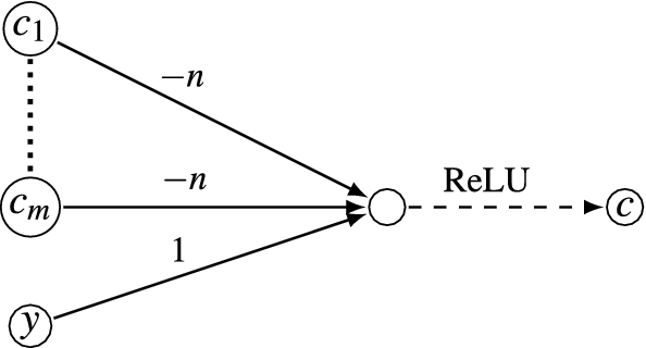
To conclude with N, the output nodes of N are $c_1,\dots ,c_m,c$. We can schematically depict N as follows:

$\square$

We also show that the complexity of the verification problem is reduced to coNP for the bounded safety fragment of $\text{bCTL}_{{\mathbb{R}}^<}$.

Corollary 2

Verifying NANES against bounded safety properties is coNP-complete in combined complexity.

Proof

The upper bound follows from the fact that we can check whether a property $\varphi = A G^k \textit{safe}$ is not satisfied by ${\mathscr{S}}$ by guessing an initial state s and a path $\rho$ of length k originating from s, and by verifying that $\rho (i) \not \models \textit{safe}$ for some $i=1,\dots ,k$. If such an initial state s exists, then there exists an initial state $s'$ with the same properties of polynomial size. This follows from the encoding into MILP and the fact that if a MILP instance is feasible, there is a solution of polynomial size.

The lower bound can be adapted from the NP lower bound of the satisfiability problem of neural networks properties [34], and holds already for one-step formulae. $\square$

Table 1 Verification times for the ${\mathscr{L}}$ properties $\varphi _{\textsf{safe}}^k$ and $\varphi _{\textsf{succ}}^k$ for different values of k on the FrozenLake scenario encoded as a NANES

7 Implementation and experiments

We have implemented the verification procedures described in the previous section in an open source toolkit called VENMAS [54]. The tool takes as input a $\text{bCTL}_{{\mathbb{R}}^<}$ specification $\varphi$ and a NANES  ${\mathscr{S}}$. The top-level call to the tool returns $\texttt {True}$ if $\varphi$ is satisfied by ${\mathscr{S}}$, and returns $\texttt {False}$ if $\varphi$ is not satisfied at some initial state of ${\mathscr{S}}$. In the latter case, a trace in the form of state-action pairs is produced, giving an example run of the system which failed to satisfy the specification.

The user provides a parameter to determine whether the monolithic or compositional procedure with parallel or sequential execution is to be used. For monolithic verification VENMAS follows Algorithm 1. For compositional verification VENMAS performs the computation in line 7 of Algorithm 2 in a splitting process that adds subprograms to a jobs queue. The computation in line 9 is performed asynchronously across a specified number of worker processes (executing on the same machine) retrieving tasks from the jobs queue: one worker process under sequential execution and multiple worker processes under parallel execution (the default in the implementation is 8). The main process finishes either when a MILP query terminates with a feasible solution (i.e., a counter-example), or all the jobs return infeasible results, or no result is returned within a given time limit.

In order to produce stronger MILP formulations, both in the case of monolithic and compositional encodings, we compute lower and upper bounds for all state and action variables. These are computed by propagating through the networks the bounds of the input states given by $I$ using symbolic interval propagation.² The bounds are used in the Big-M encoding of the ReLU nodes (see Sect. 3.2). For other kind of constraints (e.g., those expressing the transition function), the bounds are propagated using standard interval arithmetic. The bounds of the EX successor state variables are taken as the widest bounds among all possible $b$ successors.

We observe that the compositional encoding in Fig. 7 requires computing the whole set $\varPi _{{\mathscr{S}},\varphi }$ in memory, before the individual jobs can become available to the worker processes. This presents several drawbacks. First, it requires exponential memory and can be infeasible for large networks and big values of temporal depth. Second, the workers are idle at the beginning of the process. Therefore, for the experiments below, we have implemented and used a version of the compositional encoding that accepts the fragment of $\text{bCTL}_{{\mathbb{R}}^\le }$ that consists of (arbitrary) disjunctions, conjunctions over atomic propositions, and the existential path quantifier EX. The compositional encoding computes the programs in $\varPi _{{\mathscr{S}},\varphi }$ and adds them to the jobs queue one by one in a depth-first fashion. The worker processes then can start to solve verification queries as soon as individual jobs become available. If a counter-example has been detected in one of the first jobs, the whole verification procedure can terminate without computing all subproblems. Additionally, we integrated a further optimisation whereby we may discard particular jobs by examining the bounds of the state variables when encoding an atomic proposition: if the bounds (e.g., $x_1 \in [-116,-112]$) contradict the atomic formula (e.g, $(1) \ge -100$), then the whole MILP instance is trivially infeasible and no verification job is created. Finally, disjunction of atomic propositions is handled as in the monolithic case; this limits the blow-up on the number of MILPs generated whilst not hindering the efficiency of the verification procedure.

The tool is implemented in Python and uses Gurobi ver. 9.1[23] as a back-end to solve the generated MILP problems. To evaluate our tool, we performed experiments on a machine equipped with an Intel Core i7-7700K CPU @ 4.20GHz with 16GB of RAM, running Ubuntu 20.04, kernel version 5.8.

We now describe the experimental results obtained on two scenarios.

7.1 FrozenLake scenario

We started by validating VENMAS on the FrozenLake scenario from Example 1 against the specifications reported in Example 3. We considered the grid world as in Fig. 4: there are two holes – tiles ${\textsf{e}}_3$ and ${\textsf{e}}_7$, tile ${\textsf{e}}_1$ is the initial state, and tile ${\textsf{e}}_9$ is the goal.

We trained the agent’s neural network using an actor-critic approach [51]. Each training episode ends when the agent reaches the goal or falls in a hole. A reward of 1 is received if the agent reaches the goal, otherwise no reward is given. So, the agent is trained to maximise the chance of reaching the goal, including avoiding the holes. The resulting network is a ReLU-FFNN with 2 hidden layers both consisting of 32 neurons, 9 inputs and 4 outputs. The environment transition function was implemented using appropriate MILP constraints.

To evaluate how apt the agent was at realising safe and successful runs, we verified the FrozenLake system ${\mathscr{S}}_{{\textsf{f}}{\textsf{l}}}$ against the specifications $\varphi ^k_{\textsf{safe}}$ and $\varphi ^k_{\textsf{succ}}$ previously defined in Example 3, stating, respectively, that all k-bounded runs are safe and all k-bounded runs are safe and successful. To derive more optimal encodings, the specifications were equivalently formulated to minimise the number of AX operators:

$$\begin{aligned} \varphi ^k_{\textsf{safe}}= & {} \underbrace{AX \left( \texttt {ha} \ \wedge \ AX \left( \texttt {ha} \ \wedge \cdots \left( \texttt {ha} \ \wedge \ AX\texttt {ha} \right) \right) \right) }_{ k\ AX \text{'s}},\\ \varphi ^k_{\textsf{succ}}= & {} \underbrace{AX \left( \texttt {ha} \ \wedge \ AX \left( \texttt {ha} \ \wedge \cdots \left( \texttt {ha} \ \wedge \ AX\texttt {goalreached} \right) \right) \right) }_{ k\ AX \text{'s}}, \end{aligned}$$

The experiments showed that the agent was always able to avoid holes, hence to realise safe runs; however the agent was shown to be unable to ensure that the goal was reached in a given number of time steps.

Table 1 reports the time (in seconds) taken to resolve the specifications $\varphi ^{k}_{\textsf{safe}}$ and $\varphi ^{k}_{\textsf{succ}}$ for $k \in \{1, \ldots , 10\}$ for each of the execution modes. The results for the monolithic procedure are denoted Monolithic, and the results for the compositional procedure with parallel and sequential execution are denoted Comp-Par and Comp-Seq, respectively. All cases use a fixed timeout of one hour. Here we see that the compositional procedure, regardless of the execution mode, was very efficient both at finding counter-examples to $\varphi ^k_{\textsf{succ}}$ and at proving that $\varphi ^k_{\textsf{safe}}$ is satisfied. There was no difference between the sequential and parallel executions when verifying $\varphi ^k_{\textsf{safe}}$ because all jobs have been discarded by the splitting process.

The monolithic procedure also managed to locate counter-examples quickly. As for proving safety, it was significantly slower than the compositional procedure for $k \ge 6$. The main reason for this is that it produced very loose MILP formulations due to over-approximated bounds. Note that in this scenario we start from a single state; so for every program in the compositional encoding we are able to compute each next state exactly. However, in the monolithic procedure we are forced to over-approximate the bounds of the state variables $\mathbf {y}$ when encoding $EX\varphi$ since we do not know in advance which of the $b$ successors they refer to. This difficulty is further exacerbated by the discrete nature of the state space in this scenario. To see this, assume that we are in the state ${\textsf{e}}_5$, the chosen direction is down, and $\mathbf {x}$ has exact bounds (0, 0, 0, 0, 1, 0, 0, 0, 0). Then the possible successors are ${\textsf{e}}_8$, ${\textsf{e}}_4$ and ${\textsf{e}}_6$, and the bounds become very large: the upper bounds of the state variables $\mathbf {y}$ become (0, 0, 0, 1, 0, 1, 0, 1, 0) and the lower bounds all zeros. These bounds are further loosened as they are propagated through the network resulting in MILP formulations that are hard to solve.

7.2 The aircraft collision avoidance system VerticalCAS

For the second set of experiments, we consider a scenario involving two aircraft, the ownship and the intruder, where the ownship is equipped with a collision avoidance system VerticalCAS [32]. The intruder is assumed to follow a constant horizontal trajectory. Every second VerticalCAS issues vertical climbrate advisories to the ownship pilot. This is to avoid a near mid-air collision (NMAC), a region where the ownship and intruder are separated by less than 100ft vertically and 500ft horizontally. The possible advisories are:

• (1) COC: Clear Of Conflict.

• (2) DNC: Do Not Climb.

• (3) DND: Do Not Descend.

• (4) DES1500: Descend at least 1500 ft/s.

• (5) CL1500: Climb at least 1500 ft/s.

• (6) SDES1500: Strengthen Descent to at least 1500 ft/s.

• (7) SCL1500: Strengthen Climb to at least 1500 ft/s.

• (8) SDES2500: Strengthen Descent to at least 2500 ft/s.

• (9) SCL2500: Strengthen Climb to at least 2500 ft/s.

The advisories instruct the pilot to accelerate until the vertical climbrate of the ownship complies with the advisory. For some advisories, e.g. DND, the pilot can choose any acceleration in $[\frac{g}{4}, \frac{g}{3}]$, where g represents the gravitational constant 32.2 ft/s$^2$. In what follows, with slight abuse of notation, we refer to advisories using both their human readable and the corresponding numeric notation.

We hereafter denote by [m] the set $\{ 1,\ldots ,m\}$. Consider the set $\textit{S}_{\textsf{vcas}} = [-3000,3000] \times [-2500, 2500] \times [0, 40] \times [9]$. A tuple $( h, {\dot{h}}_0, \tau , \text{adv}) \in \textit{S}_{\textsf{vcas}}$ describes an ownship–intruder encounter, where:

• 1) h (ft) is the intruder altitude relative to ownship.

• 2) ${\dot{h}}_0$ (ft/s) is the ownship vertical climbrate.

• 2) $\tau$ (s) is the time to loss of horizontal separation.

• 4) $\text{adv}$ is the previous advisory issued by VerticalCAS.

Figure 8 illustrates the vertical geometry of the encounter, which is given by h and ${\dot{h}}_0$, and the time $\tau$ until the ownship (black) and intruder (red) are no longer horizontally separated.

Fig. 8

VerticalCAS encounter geometry

The VerticalCAS system is composed of nine ReLU-FFNNs $F = \left\{ \left( f_{i} : {\mathbb{R}}^3 \rightarrow {\mathbb{R}}^9 \right) : i \in [9]\right\}$, one for each advisory, with three inputs $(h,{\dot{h}}_0,\tau )$, five fully-connected hidden layers of 20 units each, and nine outputs representing the score of each possible advisory.

Table 2 Verification times for a VerticalCAS system against the property $\varphi ^k$ for different values of k and ${\dot{h}}_0$

7.2.1 NANES encoding and specification

We now formalise the VerticalCAS scenario as a NANES ${\mathscr{S}}_{\textsf{vcas}} = (\textit{Ag}_{\textsf{vcas}}, \textit{E}_{\textsf{vcas}}, I_{\textsf{vcas}})$. We model VerticalCAS as the neural agent $\textit{Ag}_{\textsf{vcas}}=(\textit{Act}_{\textsf{vcas}},\textit{prot}_{\textsf{vcas}})$ with the set of actions $\textit{Act}_{\textsf{vcas}} = [9]$ and the protocol function producing an action corresponding to the highest-scoring advisory formally defined as $\textit{prot}_{\textsf{vcas}}(s) = {{\,\mathrm{arg\,max}\,}}(\textsf{apply}(\textsf{select}(s), s))$, where for a state $s = (h, {\dot{h}}_0, \tau , \text{adv}) \in \textit{S}_{\textsf{vcas}}$:

• $\textsf{select}:\textit{S}_{\textsf{vcas}} \rightarrow F$ selects the neural network corresponding to the previous advisory $\text{adv}$, $\textsf{select}(s) = f_{\text{adv}}$;

• $\textsf{apply}:F \times {\mathbb{R}}^4 \rightarrow {\mathbb{R}}^9$ computes the output of a neural network for a given state, $\textsf{apply}(f, s) = f(h, {\dot{h}}_0, \tau )$,

• ${{\,\mathrm{arg\,max}\,}}:{\mathbb{R}}^9 \rightarrow [9]$ returns the index of the score with highest value from a neural network’s output.

Since each of the above functions and the ReLU-FFNNs are PWL, the composition $\textit{prot}$ is also PWL.

We model the ownship pilot’s non-deterministic behaviour in the environment of ${\mathscr{S}}_{\textsf{vcas}}$, defined as $\textit{E}_{\textsf{vcas}} = (\textit{S}_{\textsf{vcas}}, t_{\textit{E}_{\textsf{vcas}}})$. Thus, the environment transition function $t_{E_{\textsf{vcas}}}$ “chooses” an acceleration and determines the next state of the environment through the state transition dynamics.

The acceleration chosen by the pilot depends on the issued advisory $\text{adv}'$ and the current vertical climbrate ${\dot{h}}_0$ of the ownship. We bound the number of possible successor states of $t_{E_{\textsf{vcas}}}$ by 3, that is $b=3$, so the set of next possible accelerations is $\textit{Acc}_{\text{adv}'}^{{\dot{h}}_0} = \{\ddot{h}_0^{(1)}, \ddot{h}_0^{(2)}, \ddot{h}_0^{(3)}\}$ defined as follows. If the current vertical climbrate ${\dot{h}}_0$ of the ownship is compliant with the advisory, the pilot maintains a constant climbrate, i.e., $\ddot{h}_0^{(i)} = 0$ for $i \in [b]$. Otherwise, the pilot chooses acceleration from the continuous interval defined for each advisory. We discretise the set of possible accelerations into $b$ equally spaced cells, so for instance, $\textit{Acc}_{\text{DND}}^{{\dot{h}}_0} = \{ \frac{g}{4}, \frac{7g}{24}, \frac{g}{3} \}$.

Given the current state $s \in \textit{S}_{\textsf{vcas}}$, the issued advisory $\text{adv}' = \textit{prot}_{\textsf{vcas}}(s)$, and the set of next possible accelerations $\textit{Acc}_{\text{adv}'}^{{\dot{h}}_0} = \{\ddot{h}_0^{(i)} : i \in [b]\}$, we define each of the transition functions $t_1,\dots ,t_b$ for $t_{E_{\textsf{vcas}}}$ as:

$$\begin{aligned} t_i\left( \begin{bmatrix} h \\ {\dot{h}}_0\\ \tau \\ \text{adv} \\ \end{bmatrix}, \ \text{adv}' \right) = \begin{bmatrix} h - {\dot{h}}_0\varDelta \tau - 0.5 \ddot{h}_0^{(i)} \varDelta \tau ^2 \\ {\dot{h}}_0+ \ddot{h}_0^{(i)} \varDelta \tau \\ \tau - \varDelta \tau \\ \text{adv}' \end{bmatrix}, \end{aligned}$$

where $\varDelta \tau = 1$ and $i \in [b]$. Thus, each $t_i$ simulates a possible choice of acceleration by the pilot and computes the next state by taking into account the state transition dynamics.

The set $I_{\textsf{vcas}}$ of initial states is defined as

$$\begin{aligned} {[}-133,-129]\times {\dot{H}}_0\times \{25\}\times \{\text{COC}\}, \end{aligned}$$

where ${\dot{H}}_0 = \{-19.5 - 3k\big | k=0,\dots ,8\} \cup \{-39, -39.5, -40\}$ the set of all initial climbrates. This is a potentially risky encounter with the intruder initially below the ownship, but with the ownship descending towards the intruder.

We are interested in checking whether by following the advisories issued by VerticalCAS and independently of the acceleration chosen by the pilot, the ownship can manage to stay outside of the unsafe region ($|h| \le 100$), entering which may potentially lead to an NMAC for small values of $\tau$. So we consider the safety specifications

$$\begin{aligned} \varphi ^{k} = AX^{k} \, ((1) > 100 \ \vee \ (1) < -100) \end{aligned}$$

for various values of k. Recall that the term (1) represents the first component of the state s and so refers to h, the intruder altitude relative to ownship. Thus, the formula $\varphi ^{k}$ states that in every evolution of the system starting from every initial state in $I_{\textsf{vcas}}$ after k time steps the absolute value of vertical separation is greater than 100 ft.

7.2.2 Implementation and experiments

Our implementation of VerticalCAS system aims to compute tightest possible bounds for all states and intermediate variables in an effort to produce efficient MILP encodings.

We implemented the agent as a combination of custom MILP constraints and of NN MILP encodings. Note that in the worst case we need to choose between 9 networks to compute the action (next advisory), requiring 9 additional binary variables (similarly to encoding EX) and the constraints for each of the 9 networks. We keep the number of MILP constraints as low as possible, by avoiding to include the encodings of the networks $f_{\text{adv}}$ for advisory values that lie outside of the current bounds of the (previous) advisory variable. For instance, if these bounds identify advisory as being COC (i.e., lower and upper bounds are 1), then only the encoding of $f_{1}$ is included. This also enables computing tighter bounds for the new advisory.

The environment is implemented via a set of custom MILP constraints. Given a new advisory by the agent, we need to choose the acceleration depending on 9 possible values of the advisory. Again, we compute tight acceleration bounds by considering the bounds of the new advisory. In particular, when the latter are exact (i.e., the exact value of the advisory is known), the former are exact as well. Tight acceleration bounds allow for computing tight bounds for the next state, and so on.

We verified the VerticalCAS system ${\mathscr{S}}_{\textsf{vcas}}$ against the specifications $\varphi ^k$ for various values of k. The experiments showed that for high values of descent rate the ownship enters the unsafe region for a number of steps, eventually managing to recover. As the descent rate decreases, the time spent in the unsafe region decreases, until for the lowest value of $-19.5$ where the ownship remains safe for the entire period. For instance, the trace produced by VENMAS for ${\dot{h}}_0=-22.5$ and $k=3$ shows that the agent issues the advisory CL1500 at each time step, thereby causing the pilot to accelerate at $\frac{g}{4}$ft/s$^2$ so as to climb to avoid collision with the intruder. The descent rate was not reduced quickly enough to avoid the unsafe state $(h, {\dot{h}}_0, \tau , \text{adv}) = (-97.725,\,1.65,\,22,\,\text{CL1500})$ being reached by the third timestep.

Table 2 reports the performance of the tool in terms of time (in seconds) taken to resolve the specification $\varphi ^{k}$ for $k \in \{1, \ldots , 10\}$ with initial climbrates ${\dot{h}}_0\in {\dot{H}}_0$ for each of the execution modes. For all cases we use a fixed timeout of one hour. Here we see that the monolithic procedure is the most performant method, both for proving safety and for finding counter-examples. We attribute this to the fact that, unlike in the FrozenLake scenario, here it was possible to compute tight bounds for the state variables even after 10 time steps, resulting in tight MILP formulations whose (in)feasibility can be solved efficiently by a MILP solver. The compositional procedure was penalised as it had to construct an exponential number of programs and analyse each of them for the configurations where the property was satisfied. As before, there is no difference between sequential and parallel executions when all created subproblems have been discarded early.

We have also identified several more challenging configurations that are likely to lie close to the boundary between the safe and unsafe initial positions, such as for ${\dot{h}}_0\in \{-39, -39.5, -40, -40.5\}$ for $k\in \{9,10\}$. Because of the uncertainty, the bounds become looser. As a result, not all problems are discarded during the compositional encoding and the workers are assigned MILP problems; in this case the parallel execution is approximately twice as fast as the sequential execution. Instead, the monolithic procedure required more branch and bound iterations to find a feasible assignment or to rule out its existence. Among these initial states we also found few cases where compositional procedure was more efficient than the monolithic one (${\dot{h}}_0=-39$, $k=9$; ${\dot{h}}_0=-39.5$, $k=10$; and ${\dot{h}}_0=-40.5$, $k=9$).

Lastly, we note that we used double-precision floating point numbers for representing real values. Gurobi, the back-end MILP solver that we used, uses a default tolerance of $10^{-6}$, representing the amount of numerical error allowed on a constraint while still considering it “satisfied”. We relied on Gurobi for dealing with any further numerical issues. Finally, note that the encoding here presented is more efficient than [3], which does not compute variable bounds for their MILP encoding.

In terms of comparisons, we are unable to present an evaluation with other tools because, as far as we are aware, no other tool supports branching models and CTL specifications as we do here.

8 Conclusions

As we argued in Sect. 1, forthcoming autonomous systems will make greater use of machine learning methods; therefore there is an urgent need to develop techniques aimed at providing guarantees on the resulting behaviour of such systems. While the benefits of formal methods have long been recognised, and they have found large adoption in safety-critical systems as well as in industrial-scale software, there have been few efforts to introduce verification techniques for systems driven by neural networks.

In this paper we defined a system composed of a neural agent driven by deep feed-forward neural networks interacting with a non-deterministic environment. The resulting system displays branching evolutions. We defined and studied the resulting verification problem. While the problem is undecidable for full reachability, we isolated a fragment of the temporal language and showed that its corresponding verification problem is in coNExpTime. We developed and reported on a toolkit which includes a novel parallel algorithm to verify temporal properties of the complex environment defined in the VerticalCAS scenario. As demonstrated, while the parallel algorithm remains complete, it offers considerable advantages over its sequential counterpart when searching for counterexamples to bounded safety specifications in concrete examples.

In future work we plan to tackle scalability issues by developing alternative encodings to the ones here presented.

References

Akintunde, M., Botoeva, E., Kouvaros, P., & Lomuscio, A. (2020). Formal verification of neural agents in non-deterministic environments. In Proceedings of the 19th international conference on autonomous agents and multi-agent systems (AAMAS20) (pp. 25–33). IFAAMAS.
Akintunde, M., Kevorchian, A., Lomuscio, A., & Pirovano, E. (2019). Verification of RNN-based neural agent-environment systems. In Proceedings of the 33rd AAAI conference on artificial intelligence (AAAI19) (pp. 6006–6013). AAAI Press.
Akintunde, M., Lomuscio, A., Maganti, L., & Pirovano, E. (2018). Reachability analysis for neural agent-environment systems. In Proceedings of the 16th international conference on principles of knowledge representation and reasoning (KR18) (pp. 184–193). AAAI Press.
Anderson, R., Huchette, J., Ma, W., Tjandraatmadja, C., & Vielma, J. (2020). Strong mixed-integer programming formulations for trained neural networks. Mathematical Programming pp. 1–37.
Bastani, O., Ioannou, Y., Lampropoulos, L., Vytiniotis, D., Nori, A., & Criminisi, A. (2016). Measuring neural net robustness with constraints. In Proceedings of the 30th international conference on neural information processing systems (NIPS16) (pp. 2613–2621).
Battern, B., Kouvaros, P., Lomuscio, A., & Y. Zheng. (2021). Efficient neural network verification via layer-based semidefinite relaxations and linear cuts. In Proceedings of the 30th international joint conference on artificial intelligence (IJCAI21). To Appear. ijcai.org.
Biere, A., Cimatti, A., Clarke, E., Strichman, O., & Zhu, Y. (2003). Bounded model checking. In Highly dependable software. Advances in computers (Vol. 58). Academic Press. Pre-print.
Bordini, R., Fisher, M., Visser, W., & Wooldridge, M. (2006). Verifying multi-agent programs by model checking. Autonomous Agents and Multi-Agent Systems, 12(2), 239–256.
Botoeva, E., Kouvaros, P., Kronqvist, J., Lomuscio, A., & Misener, R. (2020). Efficient verification of neural networks via dependency analysis. In Proceedings of the 34th AAAI conference on artificial intelligence (AAAI20) (pp. 3291–3299). AAAI Press.
Bunel, R., Lu, J., Turkaslan, I., Kohli, P., Torr, P., & Mudigonda, P. (2020). Branch and bound for piecewise linear neural network verification. Journal of Machine Learning Research, 21(42), 1–39.
Cheng, C., Nührenberg, G., & Ruess, H. (2017). Maximum resilience of artificial neural networks. In International symposium on automated technology for verification and analysis (ATVA17) (pp. 251–268). Springer.
Clarke, E., Biere, A., Raimi, R., & Zhu, Y. (2001). Bounded model checking using satisfiability solving. Formal Methods in System Design, 19(1), 7–34.
Clarke, E., Grumberg, O., & Peled, D. (1999). Model checking. The MIT Press.
Doan, T., Yao, Y., Alechina, N., & Logan, B. (2014). Verifying heterogeneous multi-agent programs. In Proceedings of the 13th international conference on autonomous agents and multi-agent systems (AAMAS14) (pp. 149–156).
Dutta, S., Chen, X., & Sankaranarayanan, S. (2019). Reachability analysis for neural feedback systems using regressive polynomial rule inference. In Proceedings of the 22nd ACM international conference on hybrid systems: Computation and control (HSCC19) (pp. 157–168). ACM.
Dvijotham, K., Stanforth, R., Gowal, S., Mann, T., & Kohli, P. (2018). A dual approach to scalable verification of deep networks. arXiv preprint arXiv:1803.06567.
Ehlers, R. (2017). Formal verification of piece-wise linear feed-forward neural networks. In Proceedings of the 15th international symposium on automated technology for verification and analysis (ATVA17). Lecture notes in computer science (Vol. 10482, pp. 269–286). Springer.
Emerson, E., Mok, A., Sistla, A., & Srinivasan, J. (1992). Quantitative temporal reasoning. Real-Time Systems, 4(4), 331–352.
Fagin, R., Halpern, J., Moses, Y., & Vardi, M. (1995). Reasoning about knowledge. MIT Press.
Gammie, P., & van der Meyden, R. (2004). MCK: Model checking the logic of knowledge. In Proceedings of 16th international conference on computer aided verification (CAV04). Lecture notes in computer science (Vol. 3114, pp. 479–483). Springer.
Goodfellow, A., Bengio, Y., & Courville, A. (2016). Deep learning (Vol. 1). Cambridge: MIT press.
Griva, I., Nash, S., & Sofer, A. (2009). Linear and nonlinear optimization (Vol. 108). Siam.
Gu, Z., Rothberg, E., & Bixby, R. (2020). Gurobi optimizer reference manual. http://www.gurobi.com
Guidotti, R., Monreale, A., Ruggieri, S., Turini, F., Giannotti, F., & Pedreschi, D. (2019). A survey of methods for explaining black box models. ACM Computing Surveys, 51(5), 93:1-93:42.
Haykin, S. (1999). Neural networks: A comprehensive foundation. Prentice Hall.
Henriksen, P., & Lomuscio, A. (2020). Efficient neural network verification via adaptive refinement and adversarial search. In Proceedings of the 24th European conference on artificial intelligence (ECAI20) (pp. 2513–2520). IOS Press.
Henriksen, P., & Lomuscio, A. (2021). DEEPSPLIT: An efficient splitting method for neural network verification via indirect effect analysis. In Proceedings of the 30th international joint conference on artificial intelligence (IJCAI21). To Appear. ijcai.org.
Huang, C., Fan, J., Li, W., Chen, X., & Zhu, Q. (2019). ReachNN: Reachability analysis of neural-network controlled systems. ACM Transactions on Embedded Computing Systems (TECS), 18(106), 1–22.
Huang, X., Kroening, D., Ruan, W., Sharp, J., Sun, Y., Thamo, E., Wu, M., & Yi, X. (2020). A survey of safety and trustworthiness of deep neural networks: Verification, testing, adversarial attack and defence, and interpretability. Computer Science Reviews, 37, 100270.
Hunt, K., Sbarbaro, D., Zbikowski, R., & Gawthrop, P. (1992). Neural networks for control systems: A survey. Automatica, 28(6), 1083–1112.
Ivanov, R., Weimer, J., Alur, R., Pappas, G., & Lee, I. (2019). Verisig: Verifying safety properties of hybrid systems with neural network controllers. In Proceedings of the 22nd ACM international conference on hybrid systems: Computation and control (HSCC19) (pp. 169–178).
Julian, K., & Kochenderfer, M. (2019). A reachability method for verifying dynamical systems with deep neural network controllers. arXiv preprint arXiv:1903.00520.
Julian, K., Lopez, J., Brush, J., Owen, M., & Kochenderfer, M. (2016). Policy compression for aircraft collision avoidance systems. In Proceedings of the 35th digital avionics systems conference (DASC16) (pp. 1–10).
Katz, G., Barrett, C., Dill, D., Julian, K., & Kochenderfer, M. (2017). Reluplex: An efficient SMT solver for verifying deep neural networks. In Proceedings of the 29th international conference on computer aided verification (CAV17). Lecture notes in computer science (Vol. 10426, pp. 97–117). Springer.
Kouvaros, P., & Lomuscio, A. (2016). Parameterised verification for multi-agent systems. Artificial Intelligence, 234, 152–189.
Kouvaros, P., & Lomuscio, A. (2018). Formal verification of cnn-based perception systems. arXiv preprint arXiv:1811.11373.
Kouvaros, P., & Lomuscio, A. (2021). Towards scalable complete verification of relu neural networks via dependency-based branching. In Proceedings of the 30th international joint conference on artificial intelligence (IJCAI21). To Appear. ijcai.org.
Krizhevsky, A., Sutskever, I., & Hinton, G. (2012). Imagenet classification with deep convolutional neural networks. In Proceedings of the 25th international conference on neural information processing systems (NIPS12) (pp. 1097–1105). Curran Associates, Inc.
Liu, C., Arnon, T., Lazaru, C., Barrett, C., & Kochenderfer, M. (2019). Algorithms for verifying deep neural networks. arXiv preprint arXiv:1903.06758.
Lomuscio, A., & Maganti, L. (2017). An approach to reachability analysis for feed-forward relu neural networks. arXiv:1706.07351.
Lomuscio, A., Qu, H., & Raimondi, F. (2017). MCMAS: A model checker for the verification of multi-agent systems. Software Tools for Technology Transfer, 19(1), 9–30.
Maes, P. (1993). Modeling adaptive autonomous agents. Artificial Life, 1(1–2), 135–162.
Nair, V., & Hinton, G. (2010). Rectified linear units improve restricted Boltzmann machines. In Proceedings of the 27th international conference on machine learning (ICML10) (pp. 807–814). Omnipress.
Narodytska, N. (2018). Formal analysis of deep binarized neural networks. In Proceedings of the 27th international joint conference on artificial intelligence, (IJCAI18) (pp. 5692–5696).
OpenAI: Frozenlake-v0. https://gym.openai.com/envs/FrozenLake-v0/ (2019).
Papadimitriou, C. H., & Steiglitz, K. (1982). Combinatorial optimization: Algorithms and omplexity. Prentice-Hall Inc.
Penczek, W., & Lomuscio, A. (2003). Verifying epistemic properties of multi-agent systems via bounded model checking. Fundamenta Informaticae, 55(2), 167–185.
Redmon, J., Divvala, S., Girshick, R., & Farhadi, A. (2016). You only look once: Unified, real-time object detection. In Proceedings of the IEEE conference on computer vision and pattern recognition (CVPR16) (pp. 779–788).
Siegelmann, H., & Sontag, E. (1995). On the computational power of neural nets. Journal of Computer and System Sciences, 50(1), 132–150.
Singh, G., Gehr, T., Püschel, M., & Vechev, P. (2019). An abstract domain for certifying neural networks. In ACM on programming languages (Vol. 3, pp. 1–30). ACM Press.
Sutton, R., & Barto, A. (1998). Reinforcement learning: An introduction. MIT Press.
Szegedy, C., Zaremba, W., Sutskever, I., Bruna, J., Erhan, D., Goodfellow, I., & Fergus, R. (2014). Intriguing properties of neural networks. In Proceedings of the 2nd international conference on learning representations (ICLR14).
Tjeng, V., Xiao, K., & Tedrake, R. (2019). Evaluating robustness of neural networks with mixed integer programming. In Proceedings of the 7th international conference on learning representations (ICLR19).
VENMAS: VErification of Neural Multi-Agent Systems. https://vas.doc.ic.ac.uk/software/neural (2020).
Wang, S., Pei, K., Whitehouse, J., Yang, J., & Jana, S. (2018). Efficient formal safety analysis of neural networks. In Advances in neural information processing systems (NeurIPS18) (pp. 6367–6377).
Winston, W. (1987). Operations research: Applications and algorithms. Duxbury Press.
Xiang, W., H., Rosenfeld, J., & Johnson, T. (2018). Reachable set estimation and safety verification for piecewise linear systems with neural network controllers. In 2018 Annual American control conference (ACC) (pp. 1574–1579). AACC.
Acknowledgements
This work was partly funded by DARPA under the Assured Autonomy programme (FA8750-18-C-0095). Alessio Lomuscio is supported by a Royal Academy of Engineering Chair in Emerging Technologies.
Author information
Authors and Affiliations
Corresponding author
Additional information
Publisher's Note
Springer Nature remains neutral with regard to jurisdictional claims in published maps and institutional affiliations.
Rights and permissions
Open Access This article is licensed under a Creative Commons Attribution 4.0 International License, which permits use, sharing, adaptation, distribution and reproduction in any medium or format, as long as you give appropriate credit to the original author(s) and the source, provide a link to the Creative Commons licence, and indicate if changes were made. The images or other third party material in this article are included in the article's Creative Commons licence, unless indicated otherwise in a credit line to the material. If material is not included in the article's Creative Commons licence and your intended use is not permitted by statutory regulation or exceeds the permitted use, you will need to obtain permission directly from the copyright holder. To view a copy of this licence, visit http://creativecommons.org/licenses/by/4.0/.
About this article
Cite this article
Akintunde, M.E., Botoeva, E., Kouvaros, P. et al. Formal verification of neural agents in non-deterministic environments. Auton Agent Multi-Agent Syst 36, 6 (2022). https://doi.org/10.1007/s10458-021-09529-3
Accepted:
Published:
DOI: https://doi.org/10.1007/s10458-021-09529-3