Sedimentological data-driven bottom friction parameter estimation in modelling Bristol Channel tidal dynamics

Abstract

Accurately representing the bottom friction effect is a significant challenge in numerical tidal models. Bottom friction effects are commonly defined via parameter estimation techniques. However, the bottom friction coefficient (BFC) can be related to the roughness of the sea bed. Therefore, sedimentological data can be beneficial in estimating BFCs. Taking the Bristol Channel and Severn Estuary as a case study, we perform a number of BFC parameter estimation experiments, utilising sedimentological data in a variety of ways. Model performance is explored through the results of each parameter estimation experiment, including applications to tidal range and tidal stream resource assessment. We find that theoretically derived sediment-based BFCs are in most cases detrimental to model performance. However, good performance is obtained by retaining the spatial information provided by the sedimentological data in the formulation of the parameter estimation experiment; the spatially varying BFC can be represented as a piecewise-constant field following the spatial distribution of the observed sediment types. By solving the resulting low-dimensional parameter estimation problem, we obtain good model performance as measured against tide gauge data. This approach appears well suited to modelling tidal range energy resource, which is of particular interest in the case study region. However, the applicability of this approach for tidal stream resource assessment is limited, since modelled tidal currents exhibit a strong localised response to the BFC; the use of piecewise-constant (and therefore discontinuous) BFCs is found to be detrimental to model performance for tidal currents.

1 Introduction

Numerical modelling of tides in coastal and estuarine regions has applications in a wide variety of areas. An application of particular interest is marine renewable energy, with tidal modelling central to resource assessment for both tidal range (Adcock et al. 2015; Neill et al. 2018; Mackie et al. 2020) and tidal stream-based energy projects (Vazquez and Iglesias 2015; Wang and Yang 2020; Warder et al. 2021). With other applications of tidal models including sediment and pollutant transport (Periáñez et al. 2013; Li et al. 2018), fisheries and ecosystems (Marshall et al. 2017; Whomersley et al. 2018) and hazards such as storm surge (Flather 2000; Horsburgh and Wilson 2007; Warder et al. 2021), accurate numerical modelling of tides is highly valuable.

However, such models are subject to a variety of uncertainty sources. Modelling errors arise from assumptions and simplifications in the governing equations, as well as discretisation errors, limitations in model resolution and imperfect model inputs. One particular source of uncertainty, which is commonly addressed within the literature using parameter estimation methods, is the bottom friction coefficient (BFC). Friction between the ocean and the sea floor arises due to a boundary layer at the sea bed, and form drag due to bathymetry fluctuations. The process is not explicitly resolved in numerical models, and is instead treated as a parameterised process, via any of several formulations (Zhang et al. 2011). The value of the BFC therefore cannot be directly measured in the field, but can under certain assumptions be related to the roughness of the sea floor surface (Soulsby 1990). However, in addition to spatial variation due to bottom roughness, bottom friction parameters can also vary temporally (e.g. due to morphological changes (Davies and Robins 2017) or seasonal changes in hydrological conditions (Huybrechts et al. 2021)), as well as with mesh resolution, and a number of other physical or numerical variables (Fringer et al. 2019). For these reasons, bottom friction parameters are commonly treated via model calibration methods, where their value is determined by minimising the misfit between model outputs and observations, typically using data from tide gauges, acoustic Doppler current profilers (ADCPs) or satellite altimetry.

Approaches to model calibration within the literature vary widely in their complexity. Excluding studies dedicated to parameter estimation, the most common approach is to apply a spatially uniform BFC. In contrast, the highest-complexity approach is to allow the BFC to vary freely over the whole domain, and in this case, it is common to supplement the observation data with a form of regularisation, to avoid the problem of over-fitting (Maßmann 2010). Intermediate complexity in the friction coefficient can be achieved via several approaches. Heemink et al. (2002) divide their model domain into regions of similar influence on the model-observation misfit using an adjoint gradient-based method, also taking into account the physical properties of the system. Another more common approach is the so-called independent points scheme, where the friction coefficient field is specified by interpolation between a selected set of ‘independent points’ (Zhang et al. 2011; Chen et al. 2014). The locations of these points can be distributed uniformly or according to physical features such as the bathymetry gradient (Lu and Zhang 2006). Similarly, Sraj et al. (2014) divide their model domain by bathymetry contours in order to select a low-dimensional parameter space for their spatially varying BFC, while Mayo et al. (2014) propose the use of land use data to inform the BFC.

Alternatively, sedimentological data can be used for the purpose of constraining the spatial variation of the BFC, due to the underlying physical relationship between sediment type and the roughness of the sea bed, and hence the value of the friction coefficient. Mackie et al. (2021) directly apply Manning coefficients derived from sedimentological data within a model of the Irish Sea, supplemented by a localised BFC enhancement around a region of interest which they tune for optimal model performance. Similarly, Guillou and Thiébot (2016) utilise sedimentological data to derive a spatially varying quadratic drag parameter for a tidal stream power application off the coast of Brittany, and subsequently perform a sensitivity analysis with respect to the roughness length assigned to one of the sediment types.

Within this study, we explore the use of sedimentological data within a BFC parameter estimation problem. We perform a number of parameter estimation experiments, utilising such data in different ways. By comparing model performance using the results of each parameter estimation experiment, the objective is to arrive at recommendations regarding the use of sedimentological data in informing bottom friction parameters.

A description of the case study region, numerical model and data sources can be found in Section 2. Section 3 presents the Bayesian inference parameter estimation method used, which is based on M2 and S2 harmonic amplitude and phase data at 15 tide gauges within the model domain. Calibration and validation results can be found in Sections 4 and 5, respectively. In Section 6, we apply the calibrated model to the estimation of tidal range energy resource. The case study is primarily motivated by tidal range energy, and hence the main focus is on model comparisons with tide gauge data. However, in Section 7, we explore model performance using tidal current observations from an ADCP, as a step towards application of the calibrated model to tidal stream resource assessment. Finally, a discussion and conclusions can be found in Sections 8 and 9, respectively.

2 Description of model and data

2.1 Model study region

The model study region consists of the Bristol Channel and Severn Estuary, situated to the south-west of the UK, as shown in Fig. 1. A macrotidal inlet offering significant tidal range energy resource (Angeloudis and Falconer 2017), the Bristol Channel is also of interest for tidal stream energy (Vazquez and Iglesias 2015). Accurate tidal models of the region are also relevant to flood risk studies (e.g. Lyddon et al. (2018)) due to its susceptibility to storm surge (Proctor and Flather 1989; Williams and Horsburgh 2013). A number of flooding events have occurred in the area in recent years, for example in the Somerset Levels (Smith et al. 2017), and future flood risk is linked to climate change (Quinn et al. 2013). The region is also to be used as a case study for a calibration and validation phase of the forthcoming SWOT mission (NERC 2021).

Fig. 1

Mesh used for all simulations within this paper. Red circles: locations where harmonic analysis data are available. M2 and S2 harmonic data at these locations are used within this work for model calibration, and N2 and M4 data for validation. Yellow circles: BODC tide gauge locations, where timeseries data is available. M2 and S2 data derived from these timeseries are used within this work for validation. The coloured region of the mesh indicates where a spatially variable friction coefficient is applied

The tidal dynamics in the region are dominated by the M2 and S2 constituents, whose average amplitudes within the Bristol Channel are around 3.5 m and 1.2 m, respectively. Within this work we also utilise observations of the N2 and M4 constituents, whose amplitudes are around 0.6 and 0.2 m, respectively.

2.2 The Thetis numerical model

Within this work we use Thetis, an unstructured-mesh finite element coastal ocean model (Kärnä et al. 2018) which utilises the Firedrake finite element code generation framework (Rathgeber et al. 2016). We employ Thetis in its two-dimensional configuration (as in Vouriot et al. (2019)), which solves the nonlinear shallow water equations given by

$$ \frac{\partial \eta}{\partial t} + \nabla \cdot (H \mathbf{u}) = 0, $$

(1a)

$$ \frac{\partial \mathbf{u}}{\partial t} + \mathbf{u} \cdot \nabla \mathbf{u} + \mathbf{F_{C}} + g \nabla \eta = - \frac{\boldsymbol{\tau}_{b}}{\rho H} + \nabla \cdot (\nu (\nabla \mathbf{u} + \nabla \mathbf{u}^{T})), $$

(1b)

where η is the free surface elevation, H = η + h is the total water depth, h is the bathymetry, u is the two-dimensional depth-averaged velocity, F_C is the Coriolis force, g is the acceleration due to gravity, ρ is the water density (which is taken as a constant), τ_b is the bottom stress due to friction between the ocean and sea bed, and ν is the eddy viscosity (which we assign a constant value of 1m²s^− 1). We parameterise the bottom friction τ_b via a Manning’s n formulation

$$ \frac{\boldsymbol{\tau}_{b}}{\rho} = \frac{g n^{2}} {H^{\frac{1}{3}}}|\mathbf{u}|\mathbf{u}, $$

(2)

where n is the Manning coefficient (units s m^1/3). For the purposes of model calibration within this work, n depends on the sediment type found on the ocean bed (see Section 2.3).

Since the Bristol Channel and Severn Estuary contain significant intertidal regions, we include wetting and drying within Thetis using the scheme of Kärnä et al. (2011), which we summarise here. Under this scheme, a modification is applied dynamically to the bathymetry in order to avoid negative water depth. The modified bathymetry is given by

$$ \tilde{h} = h + f(H), $$

(3)

such that the modified water depth is similarly given by

$$ \tilde{H} = H + f(H). $$

(4)

The implementation of this scheme simply requires this modified depth $\tilde {H}$ to be substituted for H in Eq. (1a). The function f(H) is chosen such that the modified water depth $\tilde {H}$ is always positive. Following Kärnä et al. (2011), we use

$$ f(H) = \frac{1}{2} \left( \sqrt{H^{2} + \alpha^{2}} - H \right), $$

(5)

where α is a wetting-drying parameter which controls the transition from wet to dry regions, and is user defined. In general, smaller values of α result in more accurate results, but there exists a minimum stable value which is related to the mesh element size. In all Thetis simulations presented herein, α is taken to be 1 m; this value was found through preliminary experiments (not shown) to be close to the minimum stable value for the selected mesh.

Mesh generation was performed using the Python package qmesh (Avdis et al. 2018), which interfaces the mesh generator Gmsh (Geuzaine and Remacle 2009). The mesh, shown in Fig. 1, adopts a UTM30 coordinate projection, and uses a variable mesh element size from 250 m in the inner Bristol Channel, to 8 km in open regions, resulting in a total of 42,862 triangular elements. Coastline data for mesh generation is from the Global Self-consistent, Hierarchical, High-resolution Geography Database (GSHHG) (Wessel and Smith 1996). Thetis is run using a $\text {P}_{1}^{\text {DG}}$–$\text {P}_{1}^{\text {DG}}$ discretisation, with a Crank-Nicolson timestepping scheme with a timestep Δt = 100 s. The bathymetry is from 6-arcsecond resolution data available from Digimap (Digimap 2016), and is shown in Fig. 2.

Fig. 2

Top: Bathymetry over the full model domain. Bottom: Bathymetry within the Bristol Channel and Severn Estuary. Coordinates are in the UTM30 projection

Tidal dynamics are introduced through a Dirichlet boundary condition for the surface elevation η at the ocean boundary, extracted from the TPXO database (Egbert and Erofeeva 2002). The location of the ocean boundary of the model domain was selected to be in reasonably deep water, to minimise the influence of errors in this tidal boundary forcing data. The tidal dynamics within the Bristol Channel are dominated by the M2 and S2 constituents (with amplitudes in excess of 1 m), with some contribution from the N2, K2 and M4 constituents (amplitudes in the 10s of cm), and no other constituents above 10-cm amplitude. Due to their similar frequencies and the constraints of the Rayleigh criterion, the K2 and S2 constituents require long periods of observation/simulation to be resolved, and we therefore neglect the K2 constituent. The M2, S2, N2 and M4 constituents are therefore the focus of model-observation comparisons we perform within this study, and thus we use the same four constituents to force the model at its boundaries. The shallow-water M4 constituent is mostly generated within the model domain and has small amplitude on the boundaries, but is nevertheless included in the boundary forcing. Model runs span a 5-day spinup period, followed by two full spring-neap cycles (approximately 1 month).

2.3 Parameterising the Manning coefficient

We employ a parameter estimation method in order to calibrate the model with respect to the spatially varying Manning coefficient, n. In order to constrain the parameter’s spatial variation, we use sediment maps within the model domain. In an approach similar to Mackie et al. (2021), we use data from the British Geological Survey (British Geological Survey 2021), which indicates the type of sediment found at each point in the domain. The distribution of sediment types is shown in Fig. 3 and summarised in Table 1.

Fig. 3

Spatial distribution of sediment types within the Bristol Channel, from the British Geological Survey (British Geological Survey 2021). See also Table 1

Table 1 Sediment types defined by the British Geological Survey (British Geological Survey 2021), sorted by roughness length

The Manning coefficient can in principle be determined directly from the sediment type found at a given location, via a lookup table for the median sediment grain size for the corresponding sediment type. Denoting the median grain size d₅₀ (in m), the corresponding theoretical Manning coefficient is given by

$$ n(d_{50}) = 0.04 \sqrt[6]{2.5 d_{50}} $$

(6)

(Soulsby 1990). This results in the set of Manning coefficients detailed in Table 1, which are consistent with standard sediment-based values from other sources (e.g. Arcement and Schneider (1989)). Throughout this paper, we refer to the set of Manning coefficients computed via Eq. 6 as the ‘standard’ or ‘theoretical’ sediment-based parameters.

However, there is uncertainty inherent in the direct application of Manning coefficients computed as above. The bed friction term in the model governing equations must ideally account for unresolved bathymetry and bedforms, which are not accounted for within Eq. 6. Additionally, due to numerical dissipation, it may be the case that the optimal friction coefficients within a numerical model are smaller than those corresponding to the true properties of the sea bed (Fringer et al. 2019). Therefore, even when sediment data is available (as is the case here), it is common within the numerical modelling literature to perform model calibration with respect to the bottom friction coefficient. Nevertheless, the availability of sediment data can be used to constrain the spatial variation of the bottom friction parameter, in order to reduce the dimension of the parameter space for parameter estimation.

Within this work, we perform several parameter estimation experiments labelled A, B, C1 and C2 and described below. In each case, the Manning coefficient in the outer region of the model domain, indicated by the white region of the mesh in Fig. 1, is held constant at n = 0.025 sm^1/3. Since model-observation comparisons are made only within the Bristol Channel, the value for n within this outer region was found to have only a very weak influence on the model performance metrics, and a value of n = 0.025 sm^1/3 was found through preliminary experiments (not shown) to produce adequate results. The value for n inside the Bristol Channel (coloured region in Fig. 1) is described below for each experiment:

Experiment A::

Estimation of a spatially uniform Manning coefficient.

The simplest approach is to discard the sediment data entirely, and estimate only a spatially uniform Manning coefficient (i.e. a single value), n₀. This is a commonly taken approach within the literature, especially where more advanced model calibration is not directly the focus of the work.

Experiment B::

Estimation of a scaling factor for the standard sediment-based Manning coefficients.

An alternative is to scale the Manning coefficients given by Eq. 6 by a spatially uniform factor γ, such that

$$ n(d_{50}) = 0.04 \gamma \sqrt[6]{2.5 d_{50}}. $$

(7)

The parameter estimation problem is to determine the optimal value for γ. The motivation

for this approach is that the sediment-based Manning coefficient is likely to overestimate the required bottom friction, due to the presence of numerical dissipation, but that the relative values of the Manning coefficients based on the sediment data may still be appropriate. This approach results in the same number of degrees of freedom (one) in the parameter estimation problem as experiment A, but incorporates a priori knowledge about the physical process of bottom friction.

Experiment C::

Direct estimation of a small number of Manning coefficients corresponding to groups of sediment classes.

The third approach we take within this work is to estimate three Manning coefficients (n₁,n₂,n₃), each corresponding to a group of sediment types. We choose to group the sediment types into approximately equal area (see Table 1), such that n₁ corresponds to sediment types 1–4, n₂ to types 5–8, and n₃ to types 9–13. This grouping is shown in Fig. 4. While we could have used the sediment data to divide the domain into more than three subdomains, this would result in large variation in subdomain area, with parameters corresponding to small domain areas unlikely to be well constrained by the observations.

Fig. 4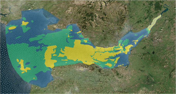

Grouping of sediment classes for the purposes of parameter estimation experiments C1 and C2. Yellow corresponds to parameter n₁, green n₂ and blue n₃. In any regions where sediment data is unavailable, the default Manning coefficient of n = 0.025 sm^1/3 is applied

We further subdivide this experiment into two. In experiment C1, we use uniform priors for each parameter within the Bayesian inference parameter estimation algorithm we employ. In experiment C2, we use the standard sediment-derived Manning coefficients to construct Gaussian prior distributions for each parameter.

Alongside the results of each of the above parameter estimation experiments, we also present results based on a uniform Manning coefficient of 0.025 sm^1/3 throughout the model domain. This value is somewhat arbitrary, but falls within the commonly used range of uniform Manning coefficients within the literature. Results using this uniform BFC represent a useful benchmark against which to compare the performance resulting from each of the above parameter estimation experiments.

2.4 Observation data

We use data from two sources for the purposes of model calibration and validation, as indicated in Fig. 1:

• 1. 15 locations at which tidal harmonic data is available (National Oceanography Centre, personal communication 2018), which are shown as red circles in Fig. 1. We use the M2 and S2 harmonic amplitudes and phases at these locations for the model calibration. N2 and M4 data at these locations are used for model validation. The tidal harmonics at each observation location were computed from tide gauge records between 1 month and 1 year in length, between 1960 and 1980.

• 2. Five tide gauges where quality controlled timeseries surface elevation data are available from the British Oceanographic Data Centre (BODC). These locations are shown in Fig. 1 by yellow circles. The tidal constituent data we use at these locations is from a harmonic analysis of observations spanning a 10-year period from 1997. We use M2 and S2 amplitude and phase observations at these locations for further validation of the calibrated models.

3 Parameter estimation method

There exist a large number of algorithms within the literature for estimating unknown bottom friction parameters. In the simple one-dimensional case (i.e. using a spatially uniform BFC), it is common to employ a simple grid search. This involves simply running the numerical model with a small number of different BFC values, and selecting the value which minimises a given measure of model-observation misfit. However, this approach scales poorly with the number of parameters to be estimated. The high-complexity approach (estimating an independent BFC value at every mesh node) typically requires numerical adjoint models, which constitute an efficient technique for evaluating gradients of model outputs (typically a functional representing the model-observation misfit) with respect to the control parameters, thus facilitating the use of gradient-based optimisation methods for performing model calibration (Maßmann 2010). The use of intermediate-complexity BFC parameterisations is compatible with a number of approaches, with adjoint (Zhang et al. 2011) or other gradient-based methods (Sraj et al. 2014), Kalman filters (Mayo et al. 2014; Siripatana et al. 2017) and Markov Chain Monte Carlo (MCMC) methods (Hall et al. 2011; Sraj et al. 2014) all employed within the literature.

Within this work, we take a Bayesian inference approach via an MCMC algorithm. We utilise a Gaussian process emulator as an efficient surrogate for the full numerical model. This is necessary because the MCMC algorithm requires large numbers of model runs (typically $\mathcal {O}(10^{6})$), which is not feasible with the full numerical model. While our numerical model does have an adjoint model available, the size of the parameter estimation problems we solve within this work is relatively small and does not warrant adjoint methods. Kalman filter approaches typically require some tuning of algorithm parameters for optimal performance (Siripatana et al. 2017). The MCMC approach however is fairly straightforward and well suited to the size of the problem considered here. Its results are simple to interpret, and also yield a direct estimate of the uncertainty in the estimated parameters.

The following exposition of the Bayesian inference algorithm proceeds for parameter estimation experiment C, since this is the most general case (estimating the greatest number of parameters). The application of the method to experiments A and B requires only minor adaptation.

3.1 Bayesian inference

Within this work, the observation data we use for calibration consists of M2 and S2 harmonic amplitudes and phases at 15 tide gauge locations (as indicated by the red circles in Fig. 1).

We denote these four observations types by j = 1,2,3,4, corresponding to M2 amplitude, S2 amplitude, M2 phase and S2 phase, respectively. The observation data is thus represented by four vectors y_j, each of length N = 15. For compactness, we denote the full set of observations Y, a matrix with shape (4 × N), whose rows are given by the vectors y_j. The corresponding model outputs for observation type j are denoted f_j(n). Bayes’ theorem gives

$$ {\Pi}(\mathbf{n}|Y) \propto L(Y|\mathbf{n}) \prod\limits_{i=1}^{3} q_{i}(n_{i}), $$

(8)

where π is the posterior distribution of the parameters n = (n₁,n₂,n₃) given the observed data Y, L is the likelihood of observing the outputs Y given the parameters n and q_i is the prior distribution for each of the parameters n_i.

The likelihood L is estimated from the numerical model. For observation type j, we assume that the model-observation discrepancies, which are the components of the vector y_j −f_j(n), are independent and identically distributed variables with zero mean and variance ${\sigma _{j}^{2}}$. The likelihood L(Y |n) is then given by

$$ L(Y|\mathbf{n}) = \prod\limits_{j=1}^{4} \left[ (2 \pi {\sigma_{j}^{2}})^{-N/2} \exp{\left( -\frac{1}{2} \frac{|\mathbf{y}_{j} - \mathbf{f}_{j}(\mathbf{n})|^{2}}{{\sigma_{j}^{2}}}\right)} \right]. $$

(9)

Since the ${\sigma _{j}^{2}}$ values are unknown a priori, they are treated as hyperparameters, i.e. they are included as additional parameters to be inferred by the inversion algorithm. We denote the full vector of unknowns $\boldsymbol {\theta } = (n_{1}, n_{2}, n_{3}, \log {{\sigma _{1}^{2}}}, \log {{\sigma _{2}^{2}}}, \log {{\sigma _{3}^{2}}}, \log {{\sigma _{4}^{2}}})$, and the full posterior distribution is therefore given by

$$ \begin{array}{@{}rcl@{}} {\Pi}(\boldsymbol{\theta}|Y) \propto && \prod\limits_{j=1}^{4} \left[ (2 \pi {\sigma_{j}^{2}})^{-N/2} \exp{\left( -\frac{1}{2} \frac{|\mathbf{y}_{j} - \mathbf{f}_{j}(\mathbf{n})|^{2}}{{\sigma_{j}^{2}}}\right)} \right] \\ && \prod\limits_{i=1}^{3} q_{i}(n_{i}) \prod\limits_{j=1}^{4} q_{j}({\log\sigma_{j}^{2}}), \end{array} $$

(10)

where $q_{j}({\log \sigma _{j}^{2}})$ is the prior distribution of ${\log \sigma ^{2}_{j}}$.

3.1.1 Priors

For parameter estimation experiments A, B and C1, we use uniform priors for the corresponding control parameters. This is equivalent to setting q_i(n_i) = 1 in Eq. 10 (the normalisation is not important). For parameter estimation experiment C2, we use the ‘standard’ sediment-based Manning coefficients of Table 1 to construct

Gaussian priors for each of the Manning coefficients. That is, the priors are given by

$$ q_{i}(n_{i}) = \frac{1}{s_{i} \sqrt{2\pi}} \exp{\left( -\frac{1}{2} \frac{(n_{i} - \mu_{i})^{2}}{{s_{i}^{2}}}\right)}, $$

(11)

where μ_i and s_i are the mean and standard deviation of the prior distributions, whose values are summarised in Table 2.

Table 2 Mean (μ) and standard deviation (s) for the Manning coefficient priors in experiment C2

For the unknown variances ${\sigma _{j}^{2}}$, the only prior constraint is that they must be positive. For all parameter estimation experiments within this study, we follow the approach of Sraj et al. (2014) and assume Jeffreys priors (Sivia and Skilling 2006), such that

$$ q_{j}({\log\sigma_{j}^{2}})= \frac{1}{{\sigma_{j}^{2}}}. $$

(12)

3.2 Markov Chain Monte Carlo algorithm

A technique for sampling the posterior distribution given by Eq. 10 is the Markov Chain Monte Carlo (MCMC) method, which has the advantage that the constant of proportionality in the equation need not be determined. We use an implementation of the Random Walk Metropolis Hastings MCMC algorithm (Hastings 1970), which is given by Algorithm 1. The algorithm requires the selection of an appropriate proposal distribution covariance matrix, Σ_step, governing the size of the random steps within the parameter space. We set

$$ {\Sigma}_{\text{step}} = \text{diag}(0.001^{2}, 0.001^{2}, 0.001^{2}, 0.1^{2}, 0.1^{2}, 0.1^{2}, 0.1^{2}) $$

(13)

so that the random steps in each of the Manning coefficients have zero mean and a standard deviation of 0.001 sm^1/3, and the random steps in each value of $\log {{\sigma _{j}^{2}}}$ have zero mean and a standard deviation of 0.1. These step sizes were found to give satisfactory results, without the need for an adaptive MCMC algorithm.

In the results presented here, we take M = 10⁶ samples, discarding the first 2 × 10⁵ as a burn-in period, and the resulting chain of values n^[k] generated by the MCMC algorithm constitute samples from the posterior distribution. The mean of these samples is taken as the best estimate of the parameter values.

3.3 Gaussian process emulation

We employ a Gaussian process emulator (GPE) as a computationally inexpensive surrogate for the full numerical model. For parameter estimation experiment C, this GPE is trained using 40 model runs with Manning coefficient samples drawn from uniform prior distributions in the range [0.01, 0.05], using Latin Hypercube Sampling to evenly sample the three-dimensional parameter space. Experiment A is a simplified version of experiment C, and can therefore utilise the same GPE. For experiment B, where the objective is to estimate the scaling parameter γ (see Eq. 7), the GPE is trained using 10 samples for γ drawn uniformly between 0.55 and 1.0, inclusive. Values for γ smaller than 0.55 resulted in model instabilities due to the very low friction coefficients in some regions. Once trained, the GPE is substituted for f(n) within the MCMC algorithm described above. Within this study, we use the Python package GPy (GPy since 2012) for the construction of GPEs.

The use of a GPE in place of the full Thetis model introduces additional uncertainty. However, this uncertainty can be directly estimated by the GPE. The GPE-introduced covariances were typically around 10^− 6 m² for emulated amplitudes, and 2 × 10^− 3∘2 for emulated phases. Since the model-observation variances (${\sigma _{j}^{2}}$ in the above description of the Bayesian inference) were typically around 25 cm² for amplitudes, and 6.25^∘2 for phases, the additional uncertainty introduced by the GPEs is small, and can be neglected.

4 Calibration results

4.1 Optimal parameters

The optimal Manning coefficient fields for each parameter estimation experiment are shown in Fig. 5. Note that in all cases, the value of the Manning coefficient outside the Bristol Channel takes a fixed value of n = 0.025 s m^1/3, as described in Section 2.3. We make further comments on the results from each experiment below.

Fig. 5

Manning coefficient fields used for model validation. a Standard sediment-based parameters. b Result of experiment A. c Result of experiment B. d Result of experiment C1. e Result of experiment C2

Experiment A::

Uniform parameter inside Bristol Channel

The optimal uniform parameter within the Channel (and its uncertainty) is given by n₀ = 0.0274 ± 0.0003. This value lies within the range of commonly used uniform parameter values in the literature.

Experiment B::

Scaling of ‘standard’ sediment-based parameters

The MCMC algorithm returns a scaling parameter γ = 0.813 ± 0.013. This is consistent with the expectation that the ‘standard’ sediment-based parameters are too strongly dissipative, due to the presence of numerical dissipation.

Experiment C1::

Three-dimensional parameter space, uniform priors

The values for each Manning coefficient returned by the MCMC algorithm are n₁ = 0.032 ± 0.002, n₂ = 0.021 ± 0.007, n₃ = 0.025 ± 0.003. The marginal posterior distributions for each parameter are shown in Fig. 6. Each marginal distribution is obtained by integrating the full posterior distribution over two of the parameters, leaving the marginal PDF for each parameter individually. The relative magnitudes of the Manning coefficients returned by this experiment are unexpected; given the sediment types corresponding to each parameter, we would expect n₁ > n₂ > n₃. We note that the posterior distribution for n₂ is very broad. The parameter estimation results are therefore not necessarily inconsistent with this expectation, but the means of the distributions do not fall in the expected order.

Experiment C2::

Three-dimensional parameter space, Gaussian priors

The values for each Manning coefficient returned by the MCMC algorithm are n₁ = 0.0317 ± 0.0016, n₂ = 0.024 ± 0.004 and n₃ = 0.0222 ± 0.0019. The marginal posterior distributions for each parameter are shown in Fig. 7, along with the prior distributions. The prior distribution for n₁ is very broad, with the observation data able to achieve a far tighter constraint. For all three parameters, the posterior distributions are narrower than for experiment C1, due to the additional constraints provided by the priors. Note also that the influence of the priors is sufficient for the parameters to fall in the expected order (n₁ > n₂ > n₃), in contrast to experiment C1.

Fig. 6

Marginal posterior distributions for each parameter n_i, from experiment C1

Fig. 7

Marginal posterior distributions for each parameter n_i, from experiment C2. Dotted lines indicate the prior distributions for each parameter

4.2 Performance against calibration dataset

In this section, we summarise the performance of the model with the Manning coefficient field resulting from each parameter estimation experiment, as measured against the calibration dataset (locations indicated by red circles in Fig. 1). Results presented here are based on runs of the full numerical model (not the GPE). The M2 and S2 amplitude and phase RMSEs achieved with each coefficient field are summarised in Table 3.

Table 3 Root mean squared errors (RMSEs) of the modelled M2 and S2 amplitudes (α) and phases (ϕ), for each Manning coefficient field, aggregated across the calibration tide gauges (red circles in Fig. 1)

As described in Section 2.3, the uniform BFC of 0.025 s m^1/3 is used as a benchmark, with which we can compare model performance using the other BFC fields. The ‘standard’ sediment-based parameters perform very poorly, with significantly greater RMSEs than the benchmark run. Experiment A (optimal uniform BFC) performs well and achieves the overall lowest amplitude and phase RMSEs for the S2 constituent, while the greatest improvement over the benchmark run is for the M2 amplitude. Experiment B does not perform as well as experiment A, suggesting that the direct use of sediment-derived coefficients (even when scaled) is detrimental to model performance. Experiments C1 and C2 both perform well. Experiment C1 performs best overall, since its RMSEs are all within 0.1 cm or 0.1^∘ of the lowest achieved in all cases. This is to be expected, since experiment C1 uses the greatest number of degrees of freedom in representing the Manning coefficient, with the fewest additional constraints (whereas experiment C2 includes Gaussian priors for the unknown parameters).

Figure 8 compares the modelled and observed M2 and S2 amplitudes and phases for both the ‘standard’ and experiment C1 cases. These results demonstrate the excessive dissipation due to the ‘standard’ friction coefficients, resulting in underestimated amplitudes. Figure 9 indicates the spatial distribution of the M2 amplitude errors within the Bristol Channel using the ‘standard’ parameters, and shows the increasing magnitude of the model errors further into the channel, where the amplitude increases due to resonance. The result of experiment C1 exhibits significantly reduced scatter in Fig. 8, corresponding to the reduced RMSEs summarised in Table 3.

Fig. 8

Scatter plots of modelled M2 and S2 amplitude and phase, against observed values. Top: using ‘standard’ sediment-based parameters. Bottom: using result from experiment C1. The ‘standard’ parameters systematically underestimate the observed amplitudes

Fig. 9

Map of M2 amplitude model errors, using the ‘standard’ parameters. The errors increase in magnitude further into the channel

5 Validation of calibrated models

Section 4.2 summarised model performance against the set of data which was used directly within the model calibration. In this section, we make additional model-observation comparisons in order to validate the calibrated models resulting from each parameter estimation experiment.

5.1 Validation using additional harmonic constituents

The parameter estimation algorithm used only the M2 and S2 amplitude and phase data at the locations indicated by red circles in Fig. 1. As described in Section 2.2, the N2 and M4 constituents have amplitudes in the

10s of cm within the model domain. These constituents are included in the model boundary condition, and can be resolved by harmonic analysis based on the 1-month model runs. We can therefore make additional comparisons between the modelled and observed amplitudes and phases for these two constituents. These RMSEs are summarised in Table 4.

Table 4 Root mean squared errors of the modelled N2 and M4 amplitudes and phases, for each Manning coefficient field, aggregated across the calibration tide gauges (red circles in Fig. 1)

The ‘standard’ sediment-based friction field produces the smallest N2 amplitude RMSE, in contrast with its poor performance on all other error metrics. The benchmark run (with uniform n = 0.025 sm^1/3) produces the smallest N2 phase errors. Experiment B produces the smallest RMSEs for the M4 amplitude, while experiment C2 produces the smallest M4 phase RMSE. As was the case for the error metrics against the calibration data, experiments C1 and C2 produce similar RMSEs. Overall, the N2 and M4 validation metrics do not strongly favour a particular parameter estimation experiment, and the N2 amplitude in particular appears difficult to model accurately.

5.2 Validation using additional tide gauge locations

In this section, we compare model outputs with data from the five BODC tide gauge locations (indicated by yellow circles in Fig. 1). Data at these locations were not used in the parameter estimation experiments.

The M2 and S2 amplitude and phase RMSEs aggregated across these five tide gauges are summarised in Table 5 for each BFC field. We find that experiment C1 produces the smallest values for all four RMSEs. Experiments A and C2 also perform well. Experiment B produces a relatively high M2 amplitude RMSE, but is still an improvement on the benchmark n = 0.025 s m^1/3 run. Model performance for the N2 and M4 constituents at these validation tide gauges follows a similar pattern to the performance at the calibration gauges, and is therefore not shown.

Table 5 Root mean squared errors of the modelled M2 and S2 amplitudes and phases, for each Manning coefficient field, aggregated across the validation tide gauges (yellow circles in Fig. 1)

These results suggest that over-fitting has not been an issue in any of the parameter estimation experiments. The N2 and M4 error metrics do not strongly favour any particular BFC configuration, while the M2 and S2 error metrics at new locations show improvements which are consistent with the corresponding error metrics against the calibration data.

Due to the similarity in the results of experiments C1 and C2, throughout the remainder of this paper, we limit our analysis to the ‘standard’ sediment-based parameters, and the results from parameter estimation experiments A, B and C1.

6 Implications for tidal range energy

In this section, we consider the mean modelled tidal range energy, and its sensitivity to the bottom friction parameterisation. At a given location, the mean tidal range energy density (or potential energy density, PED) is computed as

$$ \text{PED} = \frac{1}{M} \sum\limits_{i=1}^{M} \frac{1}{2} \rho g (HW_{i} - LW_{i})^{2}, $$

(14)

where the sum is over M = 28 semidiurnal tidal periods spanning a single complete spring-neap cycle, ρ is the density of water and HW_i and LW_i are the high and low water surface elevations from each semidiurnal cycle i, respectively. The result has units of J m^− 2 per tidal cycle.

We compute the mean tidal range energy density at each of the tide gauge locations shown in Fig. 1, using both the model (with various friction parameters) and observations. This energy density is computed

from surface elevation timeseries reconstructed from the M2 and S2 harmonic constituents, since these constituents dominate the tidal dynamics in the region and are well captured by the model. A comparison between these modelled and observed values is presented in Fig. 10. The ‘standard’ sediment parameters result in a severe underestimate of the tidal range energy density, while the other parameter sets all perform reasonably well. As shown in Table 6, experiment C1 produces the smallest tidal range energy density RMSE; this is to be expected, since it also performs best in terms of M2 and S2 amplitude and phase RMSEs.

Fig. 10

Comparison of modelled and observed mean tidal range energy density over a spring-neap cycle. The names of each tide gauge location are indicated

Table 6 Root mean squared errors (RMSEs) of the modelled mean tidal range energy densities, compared with observations at the tide gauge locations

Figure 11 shows the modelled mean tidal range energy density, computed over the entire Bristol Channel, using the BFC field from experiment C1. Figure 12 shows the difference between the modelled mean tidal range energy density for each other BFC field, and the result from BFC field C1 (we use the model result from experiment C1 as a central value for these different plots since it has the lowest RMSE with respect to the available observations). The results are consistent with those of Fig. 10, and the spatial patterns can be explained by the BFC distributions shown in Fig. 5. Figure 12a again demonstrates the under-estimation of the available tidal range energy when using the ‘standard’ sediment-based parameters. Figure 12b shows that the uniform parameter tends to overestimate the tidal range energy density compared with parameters C1, particularly in the central part of the channel. This central region largely coincides with the presence of bedrock, i.e. where the BFC within experiment A is smaller than within C1, leading to the observed difference. This pattern is largely reversed in Fig. 12c, corresponding to the difference between experiments B and C1; experiment B produces larger values for the BFC in the central rocky region than experiment C1, and therefore produces smaller modelled sea surface elevations. Towards the east end of the model domain (further upstream), the relative values of the BFCs are reversed, leading to a change in sign in the tidal range energy difference plots. Overall, these results reveal that the BFC has a somewhat localised effect on the modelled tidal range energy density, although the long tidal wavelength means that the differences in tidal range energy are much smoother than the differences between the BFC fields themselves (which are piecewise-constant and discontinuous).

Fig. 11

Mean tidal range energy density per tidal cycle, computed over the entire Bristol Channel, using friction field C1 (spatially varying calibrated parameter). This field results in the smallest RMSEs vs observed tidal range energy density, and is therefore the best estimate of the tidal range energy resource across the Bristol Channel

Fig. 12

Difference between modelled tidal range energy density: a with ‘standard’ parameters and parameters from experiment C1; b with parameters from experiments A and C1; c with parameters from experiments B and C1. Note the different colour bar ranges in each figure. We again observe that the ‘standard’ sediment-based parameters underestimate the energy density compared with the calibrated parameters, by an increasing amount further into the Channel. In contrast, the uniform coefficient produces higher energy densities in the central bedrock region of the channel, since it does not impose higher friction here

7 Modelling tidal currents

In this section, we perform further model validation using available tidal current observations, and discuss the application of the calibrated model to tidal stream resource assessment. Freely available ADCP data is relatively scarce within the study region, but here we make comparisons with ADCP data collected at Minehead (shown as a purple diamond in Fig. 14), on 30th July and 1st August 2001 (Stapleton et al. 2007; Liang et al. 2014). The ADCP measured velocity at 6 depths, and has been depth-averaged for numerical model comparisons.

Figure 13 compares modelled and observed current speeds at the ADCP deployment location, for the four model BFC configurations. In all cases, the model overestimates the current speeds. One surprising result is that the ‘standard’ sediment parameters, which previous results suggest overestimate the bottom friction, produce the greatest modelled velocity magnitudes at the ADCP location. This can be explained by inspecting the friction coefficient distributions of Fig. 5. The sediment types within the region are shown in Fig. 14, with the ADCP location indicated. The large region of high friction coefficient in the centre of the channel (corresponding to bedrock, sediment ID 1) acts to block the flow, driving higher currents along the southern edge of the model domain, where the sediments are finer and the BFC therefore smaller. This blockage effect depends on the relative friction coefficients between the bedrock region and the southern lower-friction area. Since the ADCP is situated within this lower friction region, the modelled velocities here are amplified by higher values for the bedrock friction coefficient. This explains why both the ‘standard’ sediment-based friction parameters, and the result of experiment B, produce the highest velocities at the ADCP location. For the parameters resulting from experiment C1, the BFC values are less extreme, and the blockage effect is therefore somewhat reduced. The parameters from experiment A, corresponding to a uniform BFC within the Bristol Channel, result in the best performance at the ADCP location, because the uniform BFC removes the blockage effect altogether.

Fig. 13

Comparison between models with various friction parameters, and depth-averaged current speed data at Minehead ADCP, from (Liang et al. 2014)

Fig. 14

Sediment zones, zoomed in to the central part of the channel. The purple diamond indicates the ADCP location, which lies within a region of relatively fine sediment

This is further demonstrated by Figs. 15 and 16. Figure 15 shows the mean modelled kinetic power density across the model domain, using the C1 parameters, and exhibits small-scale variability in the tidal stream resource, due mostly to bathymetric and coastline features. Similar to Fig. 12 for mean tidal range energy, Fig. 16 shows the differences between the modelled mean tidal stream power density for each BFC field, compared with the result from BFC field C1. There is high spatial correlation between these differences and the differences in the BFC fields (see Fig. 5), revealing a strongly localised effect of the BFC on the modelled tidal stream resource. In particular, Fig. 16b shows the difference in modelled mean tidal stream power density between parameters A (uniform BFC) and C1, and demonstrates the blockage effect described above, with the uniform BFC producing lower velocities in regions of finer sediment at the southern edge of the model domain.

Fig. 15

Mean tidal stream kinetic power density, computed over the entire Bristol Channel, using friction parameters from experiment C1

Fig. 16

a Difference in modelled mean tidal stream power density between ‘standard’ parameters and parameters C1. b Difference for parameters A and C1. c Difference for parameters B and C1. Similarly to the tidal range energy density, the tidal stream power density is mostly underestimated by the ‘standard’ sediment-based parameters compared with the calibrated parameters, with a particularly strong local effect in the region of bedrock in the channel centre. However, due to the blockage effect of increased friction in the centre of the channel, the kinetic energy increases at the southern edge, where the friction coefficient is smaller

Overall, the results of this section demonstrate the increased complexity of tidal currents compared with tidal elevations, with both the bathymetry and BFC having a strong localised effect on model velocities. We therefore conclude that calibration for tidal stream resource assessment requires further work. Tidal current observations spanning a broader spatial region are essential, and since currents are typically influenced by localised features that may well be underestimated in the interpolation of the bathymetry data to the unstructured mesh, the use of higher resolution in both the model mesh and the bathymetry may be needed. Furthermore, while the use of two-dimensional models is not uncommon for tidal stream energy studies (e.g. (Serhadlıoğlu et al. 2013; Mejia-Olivares et al. 2018)), the use of a three-dimensional model may be a prerequisite to capture the key dynamics governing tidal currents at energetic sites (Stansby 2006; Adcock et al. 2021).

8 Discussion

This study has compared various uses of sedimentological data within BFC parameter estimation, using the Bristol Channel and Severn Estuary as a case study region. We have performed a number of parameter estimation experiments, utilising the sedimentological data in different ways. These calibration experiments can be considered to be zero-, one- and three-dimensional parameter estimation problems.

The use of ‘standard’ sediment-derived BFC parameters can be considered zero-dimensional, since this approach does not involve the use of any tide gauge data to infer any model parameters. Instead, theoretical values for the BFC were applied directly to the numerical model, based on the median grain size of the sediment found at each point within the model domain. This resulted in excessive friction parameters, leading to underestimation of tidal amplitudes. This is consistent with the presence of numerical diffusion within the model in addition to the bottom friction term within the governing equations; the optimal model BFCs are smaller than would be expected from the physics of the bottom friction effect (Fringer et al. 2019).

Parameter estimation experiments A and B are both one-dimensional problems, but they take differing approaches. In experiment A, a spatially uniform BFC was inferred, whereas in experiment B, we took the sediment-derived BFC as a starting point, scaling the BFC by a uniform factor which was determined via the parameter estimation algorithm. Between these experiments, the uniform BFC (experiment A) produced better model performance, as measured against both the calibration and validation tide gauge data, than experiment B. This implies that scaling by a constant factor is not sufficient to compensate for the shortcomings of the theoretical sediment-derived parameters, and therefore in modelling applications where there is insufficient data for estimating more than one parameter, or such calibration is considered unnecessary, the commonly taken approach of a uniform BFC is most suitable. There may exist some function of the theoretical sediment-derived BFC (more complex than simple scaling as performed here) which can produce better model performance than a uniform BFC, but this would amount to the estimation of more than one parameter. The model performance with the optimal uniform BFC meets the recommended accuracy criteria of Williams and Esteves (2017), and we therefore conclude that the estimation of a spatially uniform BFC is sufficient for many practical purposes. This may particularly be the case when using a calibration algorithm whose computational cost increases with the number of parameters to be estimated (such as the algorithm we use in this study), and given that reducing model errors under one metric may be liable to increase errors under another metric (such as is observed in this study, where the spatially varying BFCs, calibrated using tidal elevation data alone, perform worse in terms of tidal currents).

In experiments C1 and C2, the sedimentological data was used to divide the Channel into three subdomains, corresponding to groups of sediment types, and a Bayesian inference algorithm employed to estimate the optimal BFC corresponding to each sediment group. Experiments C1 and C2 differed in their choice of prior within the Bayesian inference; experiment C1 used a uniform prior, whereas experiment C2 used Gaussian priors based on the theoretical sediment-derived BFC values. Due to the increased dimension of the parameter space for experiments C, their performance against both the calibration and validation tide gauge data was better than experiments A and B. Overall, experiment C1 produced slightly better performance than experiment C2; this is further evidence that the theoretical BFC values derived from the sediment data are spurious in the context of numerical model BFCs, which may be due to the presence of other modelling errors. Nevertheless, the sediment data provides a physically motivated decomposition of the model domain for constraining the spatial variation of the friction parameter, for applications where there is sufficient observation data to calibrate the model with more than one degree of freedom.

This study did not investigate the use of BFC parameterisations with more than three degrees of freedom. Doing so could result in greater model performance, but could encounter overfitting issues, and is ultimately limited by the available observation data. Furthermore, since calibration implicitly compensates for a broad variety of modelling errors, calibration with respect to a greater number of degrees of freedom will arguably become increasingly disconnected from the underlying physics of the bottom friction effect, thus making the sedimentological data less useful in constraining the spatial variation of the BFC. The results of this study suggest that, for small-dimensional parameter estimation problems, the use of sediment data for subdividing the model domain constitutes a practical approach.

However, we acknowledge that even for the low-dimensional parameter spaces we considered here, the calibration problem will be affected by the presence of a variety of sources of error (Green and McCave 1995; Waldman et al. 2017). These sources include assumptions made within the governing equations (e.g. the choice between two- and three-dimensional models, barotropic vs baroclinic models), discretisation errors, mesh resolution (Hasan et al. 2012), unresolved bathymetry (e.g. sandbars (Leuven et al. 2016)), other imperfect model inputs and other unresolved or parameterised processes. However, reductions in each of these uncertainties typically incur additional computational cost, and/or require a greater volume of observation/survey data. The modelling approach and assumptions we have taken in this work are typical of many tidal range energy studies (including several utilising the same Thetis numerical model (Angeloudis et al. 2018; Harcourt et al. 2019; Mackie et al. 2020; Baker et al. 2020)), and we have sought to make the most of the available data. This study has also neglected temporal dependence of the BFC, e.g. within the spring-neap cycle, and has assumed calm conditions with no wind or atmospheric pressure forcing, or the propagation of storm surges from outside the model domain. On longer time scales, differences in the timing of observations may also be significant. For example, the sedimentological data used within this study was collected between 1977 and 1993, with the tide gauge observations also spanning multiple decades, whereas the bathymetry is likely to change on time scales of years to decades due to both anthropogenic and natural causes. Any calibrated BFC field is always specific to the model configuration with which it was derived, and model calibration should always be interpreted within the context of these other sources of model error. However, the use of spatially dependent BFC is common within the literature (including within this model domain (Mackie et al. 2021)). This study has attempted to make the most of limited data, demonstrating that sedimentological data can be an effective basis for constraining spatially varying BFCs.

Within this work, we utilised M2 and S2 harmonic constituent data for model calibration. We acknowledge that the model-observation errors for these constituents are already small prior to calibration with a spatially varying BFC, given the broader context of the other modelling errors discussed above. However, this work has demonstrated that small changes in the BFC can correspond to changes in the tidal resonance, which is critical for the tidal dynamics and hence the tidal renewable energy resource. N2 and M4 data were withheld from the calibration, for the purposes of model validation. It is likely that incorporating all available data within the parameter estimation process would be beneficial, and may facilitate the estimation of a greater number of unknown parameters. We also note that the use of N2 data for validation was inconclusive in terms of differentiating model performance with each BFC field. Since the calibrated BFC fields will in part be compensating for imperfect model boundary conditions, the failure of M2- and S2-based calibration to improve the modelled N2 constituent may suggest the presence of errors in the boundary condition. It is certainly likely that calibration with respect to the boundary condition could produce additional improvements in model performance, but further investigation of this aspect is left to future work.

The results of Section 6 reveal a somewhat localised effect of the BFC on the tidal range energy resource. This highlights the need for observations in regions of interest, although this is mitigated by the relatively smooth variation of tidal sea surface elevations. However, in an application to modelling tidal stream resource, the highly spatially variable nature of currents, which are affected by local coastline and bathymetry features, exacerbates this issue. Reliable tidal stream resource assessment therefore requires higher-density observations in regions of interest. The results of this study also suggest that the use of sediment types to parameterise the spatial variation of the friction parameter may not be appropriate when tidal currents are of interest. This is because the tidal currents are affected on small spatial scales by rapid changes in the BFC. We have also observed the BFC exerting a non-local effect on the tidal currents, where the use of high values for the BFC in the centre of the Channel drives higher currents along the southern edge of the Channel, where the BFC is lower. This blockage effect results in the counter-intuitive result that the ‘standard’ sediment-based BFC field, which results in underestimated sea surface heights, actually produces the highest current speeds at an ADCP situated near the southern edge of the Channel. Model calibration for tidal currents may require an alternative approach to BFC parameterisation which avoids sharp changes in the coefficient, e.g. via smoothing of the BFC field, or avoiding piecewise-constant BFC fields entirely. This aspect requires further work, and more extensive tidal current data.

The primary focus of this study was on model calibration for tidal elevations, with an application to tidal range energy. As noted above, the modelling approach taken in this work is typical of many tidal range energy studies. However, although two-dimensional models are commonly used for tidal stream modelling (e.g. (Serhadlıoğlu et al. 2013; Mejia-Olivares et al. 2018)), we note that the accurate representation of tidal currents within and around candidate sites for marine energy (e.g. in highly energetic sites), warrants the use of three-dimensional models (Stansby 2006; Adcock et al. 2021). A direct comparison of two- and three-dimensional models for representing tidal currents in the Bristol Channel is beyond the scope of this study, and would be limited by the present availability of tidal current observation data, and in particular data that encompasses both horizontal and vertical variations in currents. Since the reduced computational cost of two-dimensional models offers a significant advantage to calibration studies, further work investigating the applicability of calibrated BFC fields between two- and three-dimensional models might be valuable. However, since calibration in part implicitly compensates for unresolved dynamics and modelling errors, any such applicability is likely to be limited. However, the methodology of this work, based on the use of sedimentological data for informing the spatial distribution of BFC parameters, may be applicable to three-dimensional models. Given the multiple scales that must be accounted for in marine energy hydrodynamics, the calibration of far-field two-dimensional models is also likely to maintain a role as we move to 3D, in providing boundary conditions for more computationally intensive assessments, which may need to be reserved for near-field simulations.

9 Conclusions

This study has utilised sedimentological data within a numerical model of the Bristol Channel and Severn Estuary, in order to calibrate the model against available tide gauge data. The direct use of theoretical Manning coefficient values corresponding to the median grain size for each sediment type results in severe underestimates of the sea surface height, and consequently the tidal range energy resource. This can be improved by the reduction of these theoretical BFCs by scaling with a uniform factor, with the factor determined via a Bayesian inference algorithm. However, the resulting model performance can be further improved by the use of a well-selected spatially uniform BFC, confirming that when the data or computational resources permit the solution of only a one-dimensional parameter estimation problem, the spatially uniform BFC approach remains the best option.

However, the results have demonstrated that the sedimentological data can be used to produce a piecewise-constant BFC according to three groups of sediment types. The solution of the resulting three-dimensional parameter estimation problem results in significant improvements in model performance over the uniform-BFC case, as measured against both the calibration and validation tide gauge data.

The application of the numerical model to tidal range resource assessment reveals a somewhat localised sensitivity to the BFC, highlighting the need for observation data in regions of interest. Due to the smaller-scale spatial variation in tidal currents, this issue is greater for tidal stream resource assessment, and we have also identified a non-local effect where excessive BFC values in the centre of the channel drive spuriously high currents in other regions. Further work is required for tidal stream energy applications. Such studies will require a greater volume of ADCP data that is strategically acquired. Alongside this direction, we also identify two key aspects of future modelling work which should be undertaken for tidal stream energy applications, namely the use of higher resolution in both the model mesh and bathymetry data, and further exploration of two- and three-dimensional approaches.

References

Adcock TAA, Draper S, Nishino T (2015) Tidal power generation–A review of hydrodynamic modelling. Proceedings of the Institution of Mechanical Engineers, Part A: Journal of Power and Energy 229 (7):755–771. https://doi.org/10.1177/0957650915570349
Adcock TAA, Draper S, Willden RHJ, Vogel CR (2021) The fluid mechanics of tidal stream energy conversion. Ann Rev Fluid Mech 53:287–310. https://doi.org/10.1146/annurev-fluid-010719-060207
Angeloudis A, Falconer RA (2017) Sensitivity of tidal lagoon and barrage hydrodynamic impacts and energy outputs to operational characteristics. Renew Energy 114:337–351. https://doi.org/10.1016/j.renene.2016.08.033
Angeloudis A, Kramer SC, Avdis A, Piggott MD (2018) Optimising tidal range power plant operation. Applied Energy 212:680–690. https://doi.org/10.1016/j.apenergy.2017.12.052
Arcement GJ, Schneider VR (1989) Guide for selecting Manning’s roughness coefficients for natural channels and flood plains
Avdis A, Candy AS, Hill J, Kramer SC, Piggott MD (2018) Efficient unstructured mesh generation for marine renewable energy applications. Renew Energy 116:842–856. https://doi.org/10.1016/j.renene.2017.09.058
Baker AL, Craighead RM, Jarvis EJ, Stenton HC, Angeloudis A, Mackie L, Avdis A, Piggott MD, Hill J (2020) Modelling the impact of tidal range energy on species communities. Ocean & Coastal Management 193:105221. https://doi.org/10.1016/j.ocecoaman.2020.105221
British Geological Survey (2021) Seabed sediments 250K https://www.bgs.ac.uk/datasets/marinesediments-250k/
Chen H, Cao A, Zhang J, Miao C, Lv X (2014) Estimation of spatially varying open boundary conditions for a numerical internal tidal model with adjoint method. Math Comput Simul 97:14–38. https://doi.org/10.1016/J.MATCOM.2013.08.005
Davies AG, Robins PE (2017) Residual flow, bedforms and sediment transport in a tidal channel modelled with variable bed roughness. Geomorphology 295:855–872. https://doi.org/10.1016/j.geomorph.2017.08.029
Digimap (2016) Marine themes digital elevation model 1 arc second [ASC geospatial data], Scale 1:50000, Tiles: 5050510045, 5050510050, 5051010030, 5051010035, 5051010040, 5051010045, 5051010050, 5051510025, 5051510030, 5051510035, 5051510040, 5051510045, 5051510050, Updated: 9 September 2016, OceanWise, Using: EDINA Marine Digimap Service, https://digimap.edina.ac.uk
Egbert GD, Erofeeva SY (2002) Efficient inverse modeling of barotropic ocean tides. Journal of Atmospheric and Oceanic Technology 19(2):183–204. https://doi.org/10.1175/1520-0426(2002)019<0183:EIMOBO>2.0.CO;2
Flather RA (2000) Existing operational oceanography. Coast Eng 41(1–3):13–40. https://doi.org/10.1016/S0378-3839(00)00025-9
Fringer OB, Dawson CN, He R, Ralston DK, Zhang YJ (2019) The future of coastal and estuarine modeling: findings from a workshop. Ocean Modelling 143:101458. https://doi.org/10.1016/j.ocemod.2019.101458
Geuzaine C, Remacle JF (2009) Gmsh: A 3-D finite element mesh generator with built-in pre- and post-processing facilities. Int J Numer Methods Eng 79(11):1309–1331. https://doi.org/10.1002/nme.2579, available at 1010.1724
GPy (since 2012) GPy: a Gaussian process framework in python. http://github.com/SheffieldML/GPy
Green MO, McCave IN (1995) Seabed drag coefficient under tidal currents in the eastern Irish Sea. Journal of Geophysical Research: Oceans 100(C8):16057–16069. https://doi.org/10.1029/95JC01381
Guillou N, Thiébot J (2016) The impact of seabed rock roughness on tidal stream power extraction. Energy 112:762–773. https://doi.org/10.1016/j.energy.2016.06.053
Hall JW, Manning LJ, Hankin RKS (2011) Bayesian calibration of a flood inundation model using spatial data. Water Resour Res 47(5):1–14. https://doi.org/10.1029/2009WR008541
Harcourt F, Angeloudis A, Piggott MD (2019) Utilising the flexible generation potential of tidal range power plants to optimise economic value. Appl Energy 237:873–884. https://doi.org/10.1016/j.apenergy.2018.12.091
Hasan GJ, van Maren DS, Cheong HF (2012) Improving hydrodynamic modeling of an estuary in a mixed tidal regime by grid refining and aligning. Ocean Dyn 62(3):395–409. https://doi.org/10.1007/s10236-011-0506-4
Hastings WK (1970) Monte Carlo sampling methods using Markov chains and their applications. Biometrika 57(1):97–109
Heemink AW, Mouthaan EEA, Roest MRT, Vollebregt EAH, Robaczewska KB, Verlaan M (2002) Inverse 3D shallow water flow modelling of the continental shelf. Cont Shelf Res 22:465–484. https://doi.org/10.1016/S0278-4343(01)00071-1
Horsburgh KJ, Wilson C (2007) Tide-surge interaction and its role in the distribution of surge residuals in the North Sea. J Geophys Res 112:8. https://doi.org/10.1029/2006JC004033
Huybrechts N, Smaoui H, Orseau S, Tassi P, Klein F (2021) Automatic calibration of bed friction coefficients to reduce the influence of seasonal variation: case of the Gironde estuary. J Waterw Port Coast Ocean Eng 147(3):05021004. https://doi.org/10.1061/(ASCE)WW.1943-5460.0000632
Kärnä T, de Brye B, Gourgue O, Lambrechts J, Comblen R, Legat V, Deleersnijder E (2011) A fully implicit wetting-drying method for DG-FEM shallow water models, with an application to the Scheldt Estuary. Comput Methods Appl Mech Eng 200(5–8):509–524. https://doi.org/10.1016/j.cma.2010.07.001
Kärnä T, Kramer SC, Mitchell L, Ham DA, Piggott MD, Baptista AM (2018) Thetis coastal ocean model: Discontinuous Galerkin discretization for the three-dimensional hydrostatic equations. Geosci Model Dev 11(11):4359–4382. https://doi.org/10.5194/gmd-11-4359-2018
Leuven JRFW, Kleinhans MG, Weisscher SAH, Van der Vegt M (2016) Tidal sand bar dimensions and shapes in estuaries. Earth-science reviews 161:204–223. https://doi.org/10.1016/j.earscirev.2016.08.004
Li X, Plater A, Leonardi N (2018) Modelling the transport and export of sediments in macrotidal estuaries with eroding salt marsh. Estuar Coasts 41(6):1551–1564. https://doi.org/10.1007/s12237-018-0371-1
Liang D, Xia J, Falconer RA, Zhang J (2014) Study on tidal resonance in Severn Estuary and Bristol Channel. Coast Eng J 56(01):1450002. https://doi.org/10.1142/S0578563414500028
Lu X, Zhang J (2006) Numerical study on spatially varying bottom friction coefficient of a 2D tidal model with adjoint method. Cont Shelf Res 26(16):1905–1923. https://doi.org/10.1016/J.CSR.2006.06.007
Lyddon C, Brown JM, Leonardi N, Plater AJ (2018) Uncertainty in estuarine extreme water level predictions due to surge-tide interaction. PloS ONE 13(10):e0206200. https://doi.org/10.1371/journal.pone.0206200
Mackie L, Coles D, Piggott M, Angeloudis A (2020) The potential for tidal range energy systems to provide continuous power: a UK case study. Journal of Marine Science and Engineering 8(10):780. https://doi.org/10.3390/jmse8100780
Mackie L, Evans PS, Harrold MJ, Tim ODoherty, Piggott MD, Angeloudis A (2021) Modelling an energetic tidal strait: investigating implications of common numerical configuration choices. Appl Ocean Res 108:102494. https://doi.org/10.1016/j.apor.2020.102494
Marshall KN, Kaplan IC, Hodgson EE, Hermann A, Busch DS, McElhany P, Essington TE, Harvey CJ, Fulton EA (2017) Risks of ocean acidification in the California Current food web and fisheries: ecosystem model projections. Glob Chang Biol 23(4):1525–1539. https://doi.org/10.1111/gcb.13594
Maßmann S (2010) Tides on unstructured meshes, Ph.D. Thesis, Universitat Bremen
Mayo T, Butler T, Dawson C, Hoteit I (2014) Data assimilation within the advanced circulation (ADCIRC) modeling framework for the estimation of Manning’s friction coefficient. Ocean Modelling 76:43–58. https://doi.org/10.1016/j.ocemod.2014.01.001
Mejia-Olivares CJ, Haigh ID, Wells NC, Coles DS, Lewis MJ, Neill SP (2018) Tidal-stream energy resource characterization for the Gulf of California, Mexico. Energy 156:481–491. https://doi.org/10.1016/j.energy.2018.04.074
Neill SP, Angeloudis A, Robins PE, Walkington I, Ward SL, Masters I, Lewis MJ, Piano M, Avdis A, Piggott MD, et al. (2018) Tidal range energy resource and optimization–Past perspectives and future challenges. Renew Energy 127:763–778. https://doi.org/10.1016/j.renene.2018.05.007
NERC (2021) Surface Water and Ocean Topography (SWOT) satellite calibration and validation (cal/val). https://nerc.ukri.org/research/funded/programmes/surface-water-and%-ocean-topography-swot/, accessed 17/06/2021
Periáñez R, Casas-Ruíz M, Bolívar JP (2013) Tidal circulation, sediment and pollutant transport in Cádiz Bay (SW Spain): a modelling study. Ocean Eng 69:60–69. https://doi.org/10.1016/j.oceaneng.2013.05.016
Proctor R, Flather RA (1989) Storm surge prediction in the Bristol Channel–the floods of 13 December 1981. Cont Shelf Res 9(10):889–918. https://doi.org/10.1016/0278-4343(89)90064-2
Quinn N, Bates PD, Siddall M (2013) The contribution to future flood risk in the Severn Estuary from extreme sea level rise due to ice sheet mass loss. Journal of Geophysical Research: Oceans 118 (11):5887–5898. https://doi.org/10.1002/jgrc.20412
Rathgeber F, Ham DA, Mitchell L, Lange M, Luporini F, McRae ATT, Bercea GT, Markall GR, Kelly PHJ (2016) Firedrake: automating the finite element method by composing abstractions. ACM Trans Math Softw 43:3. https://doi.org/10.1145/2998441, available at 1501.01809
Serhadlıoğlu S, Adcock Thomas AA, Houlsby GT, Draper S, Borthwick AGL (2013) Tidal stream energy resource assessment of the Anglesey Skerries. International Journal of Marine Energy 3:e98–e111. https://doi.org/10.1016/j.ijome.2013.11.014
Siripatana A, Mayo T, Sraj I, Knio O, Dawson C, Le Maitre O, Hoteit I (2017) Assessing an ensemble Kalman filter inference of Manning’s n coefficient of an idealized tidal inlet against a polynomial chaos-based MCMC. Ocean Dyn 67(8):1067–1094. https://doi.org/10.1007/s10236-017-1074-z
Sivia D, Skilling J (2006) Data analysis: a Bayesian tutorial, OUP Oxford
Smith A, Porter JJ, Upham P (2017) We cannot let this happen again: reversing UK flood policy in response to the Somerset Levels floods, 2014. J Environ Plan Manag 60(2):351–369. https://doi.org/10.1080/09640568.2016.1157458
Soulsby RL (1990) Tidal current boundary layers, The Sea, Part 1, Edited by: B. Le Méhauté, University of Miami, USA, John Wiley & Sons Inc., Printed in USA, ISBN: 0 471 63393 3
Sraj I, Iskandarani M, Carlisle Thacker W, Srinivasan A, Knio OM (2014) Drag parameter estimation using gradients and hessian from a polynomial chaos model surrogate. Mon Weather Rev 142(2):933–941. https://doi.org/10.1175/MWR-D-13-00087.1
Sraj I, Mandli KT, Knio OM, Dawson CN, Hoteit I (2014) Uncertainty quantification and inference of Manning’s friction coefficients using DART buoy data during the Tōhoku tsunami. Ocean Modelling 83:82–97. https://doi.org/10.1016/j.ocemod.2014.09.001
Stansby PK (2006) Limitations of depth-averaged modeling for shallow wakes. J Hydraul Eng 132(7):737–740. https://doi.org/10.1061/(ASCE)0733-9429(2006)132:7(737)
Stapleton CM, Wyer MD, Kay D, Bradford M, Humphrey N, Wilkinson J, Lin B, Yang L, Falconer RA, Watkins J, et al. (2007) Fate and transport of particles in estuaries: Volume iv: Numerical modelling for bathing water enterococci estimation in the severn estuary
Vazquez A, Iglesias G (2015) LCOE (levelised cost of energy) mapping: a new geospatial tool for tidal stream energy. Energy 91:192–201. https://doi.org/10.1016/j.energy.2015.08.012
Vouriot CVM, Angeloudis A, Kramer SC, Piggott MD (2019) Fate of large-scale vortices in idealized tidal lagoons. Environmental Fluid Mechanics 19(2):329–348. https://doi.org/10.1007/s10652-018-9626-4
Waldman S, Baston S, Nemalidinne R, Chatzirodou A, Venugopal V, Side J (2017) Implementation of tidal turbines in MIKE 3 and Delft3D models of Pentland Firth & Orkney Waters. Ocean & Coastal Management 147:21–36. https://doi.org/10.1016/j.ocecoaman.2017.04.015
Wang T, Yang Z (2020) A tidal hydrodynamic model for Cook Inlet, Alaska, to support tidal energy resource characterization. Journal of Marine Science and Engineering 8(4):254. https://doi.org/10.3390/jmse8040254
Warder SC, Kramer SC, Piggott MD (2021) Non-deterministic effects in modelling the tidal currents in a high-energy coastal site
Warder SC, Horsburgh KJ, Piggott MD (2021) Adjoint-based sensitivity analysis for a numerical storm surge model. Ocean Modelling 160:101766. https://doi.org/10.1016/j.ocemod.2021.101766
Wessel P, Smith WHF (1996) A global, self-consistent, hierarchical, high-resolution shoreline database. Journal of Geophysical Research: Solid Earth 101(B4):8741–8743. https://doi.org/10.1029/96JB00104
Whomersley P, Van der Molen J, Holt D, Trundle C, Clark S, Fletcher D (2018) Modeling the dispersal of spiny lobster (Palinurus elephas) larvae: implications for future fisheries management and conservation measures. Frontiers in Marine Science 5:58. https://doi.org/10.3389/fmars.2018.00058
Williams JA, Horsburgh KJ (2013) Evaluation and comparison of the operational Bristol Channel model storm surge suite, National Oceanography Centre
Williams JJ, Esteves LS (2017) Guidance on setup, calibration, and validation of hydrodynamic, wave, and sediment models for shelf seas and estuaries. Advances in Civil Engineering. https://doi.org/10.1155/2017/5251902
Zhang J, Lu X, Wang P, Wang YP (2011) Study on linear and nonlinear bottom friction parameterizations for regional tidal models using data assimilation. Cont Shelf Res 31(6):555–573. https://doi.org/10.1016/J.CSR.2010.12.011
Acknowledgements
We acknowledge the Research Computing Service at Imperial College London for HPC resources and support. This study uses data from the National Tidal and Sea Level Facility, provided by the British Oceanographic Data Centre and funded by the Environment Agency.
Funding
We acknowledge funding from the EPSRC, through the Centre for Doctoral Training in Fluid Dynamics across Scales (Grant EP/L016230/1), and grants EP/R029423/1 and EP/R511547/1. A. Angeloudis acknowledges the support of the NERC Industrial Innovation fellowship grant NE/R013209/2.
Author information
Authors and Affiliations
Corresponding author
Ethics declarations
Conflict of interest
The authors declare no competing interests.
Additional information
Responsible Editor: Zhiyu Liu
Publisher’s Note
Springer Nature remains neutral with regard to jurisdictional claims in published maps and institutional affiliations.
Rights and permissions
Open Access This article is licensed under a Creative Commons Attribution 4.0 International License, which permits use, sharing, adaptation, distribution and reproduction in any medium or format, as long as you give appropriate credit to the original author(s) and the source, provide a link to the Creative Commons licence, and indicate if changes were made. The images or other third party material in this article are included in the article's Creative Commons licence, unless indicated otherwise in a credit line to the material. If material is not included in the article's Creative Commons licence and your intended use is not permitted by statutory regulation or exceeds the permitted use, you will need to obtain permission directly from the copyright holder. To view a copy of this licence, visit http://creativecommons.org/licenses/by/4.0/.
About this article
Cite this article
Warder, S.C., Angeloudis, A. & Piggott, M.D. Sedimentological data-driven bottom friction parameter estimation in modelling Bristol Channel tidal dynamics. Ocean Dynamics 72, 361–382 (2022). https://doi.org/10.1007/s10236-022-01507-x
Received:
Accepted:
Published:
Issue Date:
DOI: https://doi.org/10.1007/s10236-022-01507-x