Flops and clusters in the homological minimal model programme

Abstract

Suppose that $f:X\rightarrow \mathrm{Spec}\,R$ is a minimal model of a complete local Gorenstein 3-fold, where the fibres of f are at most one dimensional, so by Van den Bergh (Duke Math J 122(3):423–455, 2004) there is a noncommutative ring $\Lambda$ derived equivalent to X. For any collection of curves above the origin, we show that this collection contracts to a point without contracting a divisor if and only if a certain factor of $\Lambda$ is finite dimensional, improving a result of Donovan and Wemyss (Contractions and deformations, arXiv:1511.00406). We further show that the mutation functor of Iyama and Wemyss (Invent Math 197(3):521–586, 2014, §6) is functorially isomorphic to the inverse of the Bridgeland–Chen flop functor in the case when the factor of $\Lambda$ is finite dimensional. These results then allow us to jump between all the minimal models of $\mathrm{Spec}\,R$ in an algorithmic way, without having to compute the geometry at each stage. We call this process the Homological MMP. This has several applications in GIT approaches to derived categories, and also to birational geometry. First, using mutation we are able to compute the full GIT chamber structure by passing to surfaces. We say precisely which chambers give the distinct minimal models, and also say which walls give flops and which do not, enabling us to prove the Craw–Ishii conjecture in this setting. Second, we are able to precisely count the number of minimal models, and also give bounds for both the maximum and the minimum numbers of minimal models based only on the dual graph enriched with scheme theoretic multiplicity. Third, we prove a bijective correspondence between maximal modifying R-module generators and minimal models, and for each such pair in this correspondence give a further correspondence linking the endomorphism ring and the geometry. This lifts the Auslander–McKay correspondence to dimension three.

1 Introduction

1.1 Setting

One of the central problems in the birational geometry of 3-folds is to construct, given a suitable singular space $\mathrm{Spec}\,R$, all its minimal models $X_i\rightarrow \mathrm{Spec}\,R$ and to furthermore pass between them, via flops, in an effective manner.

The classical geometric method of producing minimal models is to take Proj of an appropriate graded ring. It is known that the graded ring is finitely generated, so this method produces a variety equipped with an ample line bundle. However, for many purposes this ample bundle does not tell us much information, and one of the themes of this paper, and also other homological approaches in the literature, is that we should be aiming for a much larger (ideally tilting) bundle, one containing many summands, whose determinant bundle recovers the classically obtained ample bundle. These larger bundles, and their noncommutative endomorphism rings, encode much more information about the variety than simply the ample bundle does.

At the same time, passing between minimal models in an effective way is also a rather hard problem in general. There are various approaches to this; one is to hope for some form of GIT chamber decomposition in which wandering around, crashing through appropriate walls, eventually yields all the projective minimal models. Another is just to find a curve, flop, compute all the geometry explicitly, and repeat. Neither is ideal, since both usually require a tremendous amount of calculation. For example the GIT method needs first a calculation of the chamber structure, then second a method to determine what happens when we pass through a wall. Without additional information, and without just computing both sides, standing in any given chamber it is very hard to tell which wall to crash through next in order to obtain a new minimal model.

The purpose of this paper is to demonstrate, in certain cases where we have this larger tilting bundle, that the extra information encoded in the endomorphism ring can be used to produce a very effective homological method to pass between the minimal models, both in detecting which curves are floppable, and also in producing the flop. As a consequence, this then supplies us with the map to navigate the GIT chambers, and the much finer control that this map gives means that our results imply (but are not implied by) many results in derived category approaches to GIT, braiding of flops, and faithful group actions. We outline only some in this paper, as there are a surprising number of other corollaries.

1.2 Overview of the algorithm

We work over $\mathop {{}_{}\mathbb {C}}\nolimits$. Throughout this introduction, for simplicity of the exposition, the initial geometric input is a crepant projective birational morphism $X\rightarrow \mathrm{Spec}\,R$, with one dimensional fibres, where R is a three dimensional normal Gorenstein complete local ring and X has only Gorenstein terminal singularities. This need not be a flopping contraction, X need not be a minimal model, and R need not have isolated singularities. We remark that many of our arguments work much more generally than this, see Sect. 1.5.

Given this input, we associate a noncommutative ring $\Lambda :=\mathrm{End}_R(N)$ for some reflexive R-module N, and a derived equivalence

$$\begin{aligned} \Psi _X :\mathrm{{D}^b}(\mathrm{coh}\,X)\rightarrow \mathrm{{D}^b}(\hbox {mod}\,\Lambda ) \end{aligned}$$

(1.A)

as described in [49, §3].

It is not strictly necessary, but it is helpful to keep in mind, that a presentation of $\Lambda$ as a quiver with relations can be obtained by replacing every curve above the origin by a dot ($=$vertex), and just as in the two-dimensional McKay correspondence we add an additional vertex corresponding to the whole scheme–theoretic fibre. We draw arrows between the vertices if the curves intersect, and there are rules that establish how the additional vertex connects to the others. The loops on vertices correspond to self-extension groups, and so in the case that X is smooth, the loops encode the normal bundle of the curves. This is illustrated in Fig. 1, but for details see Sect. 2.2.

Fig. 1

From geometry to algebra

At its heart, this paper contains two key new ideas. The first is that certain factors of the algebra $\Lambda$ encode noncommutative deformations of the curves, and thus detects which curves are floppable. The second is that when curves flop we should not view the flop as a variation of GIT, rather we should view the flop as a change in the algebra (via a universal property) whilst keeping the GIT stability constant. See 1.3. Specifically, we prove that the mutation functor of [23, §6] is functorially isomorphic to the inverse of the Bridgeland–Chen flop functor [5, 10] when the curves are floppable. It is viewing the flop via this universal property that gives us the new extra control over the process; indeed it is the mutated algebra that contains exactly the information needed to iterate, without having to explicitly calculate the geometry at each step.

This new viewpoint, and the control it gives, in fact implies many results in GIT, specifically chamber structures and wall crossing, and also many results in the theory of noncommutative minimal models, in particular producing an Auslander–McKay correspondence in dimension three. We describe the GIT results in Sect. 1.3, and the other results in Sect. 1.4. In the remainder of this subsection we sketch the algorithm that jumps between the minimal models of $\mathrm{Spec}\,R$. The process, which we call the Homological MMP, is run as illustrated in Fig. 2 on page 5.

Fig. 2

The Homological MMP, jumping between minimal models

The initial input is the crepant morphism $X\rightarrow \mathrm{Spec}\,R$ above, where X has only Gorenstein terminal singularities.

Step 1: Contractions The first task is to determine which subsets of the curves contract to points without contracting a divisor, and can thus be flopped. Although this is usually obvious at the input stage (we generally understand the initial input), it becomes important after the flop if we are to continue running the programme.

Let C be the scheme-theoretic fibre above the unique closed point of $\mathrm{Spec}\,R$, so that taking the reduced scheme structure we obtain $\bigcup _{i=1}^n C_i$ with each $C_i\cong \mathbb {P}^1$. We pick a subset of the curves, say $I\subseteq \{1,\ldots ,n\}$, and ask whether $\bigcup _{i\in I}C_i$ contracts to a point without contracting a divisor. Corresponding to each curve $C_i$ is an idempotent $e_i$ in the algebra $\Lambda :=\mathrm{End}_R(N)$ from (1.A), and we set $\Lambda _I:= \Lambda /\Lambda (1-\sum _{i\in I}e_i)\Lambda$. Our first main result, a refinement of [16], is the following.

Theorem 1.1

($=$ 3.5) $\bigcup _{i\in I}C_i$ contracts to a point without contracting a divisor if and only if $\dim _\mathbb {C}\Lambda _I<\infty$.

In fact 1.1 is true regardless of the singularities on X and $\mathrm{Spec}\,R$, and needs no assumptions on crepancy. Contracting the curves $\bigcup _{i\in I}C_i$, which we can do at will since R is complete local, yields a diagram

(1.B)

By [16] there is a contraction algebra $\mathrm {A}_{\mathrm {con}}$, constructed with respect to the morphism g, that detects whether the curves in I contract to a point without contracting a divisor. The subtlety in the proof of 1.1 is that $\Lambda$ and thus $\Lambda _I$ is constructed with respect to the morphism f, so to establish 1.1 requires us to relate the algebras $\mathrm {A}_{\mathrm {con}}$ and $\Lambda _I$. It turns out that they are isomorphic, but this can only be established by appealing to a universal property. There is not even any obvious morphism between them.

Step 2: Mutation and flops We again pick a subset of curves $\{ C_i\mid i\in I\}$, but for simplicity in this introduction we assume that there is only one curve $C_i$ (i.e. $I=\{i\}$), although this paper does also cover the general situation, and all of the theorems stated here have multi–curve analogues. The curve $C_i$ corresponds to an indecomposable summand $N_i$ of the R-module N. By Step 1 the curve $C_i$ flops if and only if $\dim _{\mathbb {C}}\Lambda _i<\infty$. Regardless of whether it flops or not, we can always categorically mutate the module N with respect to the summand $N_i$, in the sense of [23, §6], to produce another module $\upnu _i N$ (possibly equal to N), together with a derived equivalence

$$\begin{aligned} \Phi _i:\mathrm{{D}^b}(\hbox {mod}\,\Lambda )\rightarrow \mathrm{{D}^b}(\hbox {mod}\,\upnu _i\Lambda ) \end{aligned}$$

where $\upnu _i\Lambda :=\mathrm{End}_R(\upnu _i N)$. See Sect. 2.3 for definitions and details. This requires no assumptions on the singularities of X, but does require R to be normal Gorenstein. Note that the categorical mutation used here is inspired by, but in many ways is much different than, the mutation in cluster theory and elsewhere in the literature. The main point is that the mutation here tackles the situation where there are loops, 2-cycles, and no superpotential, which is the level of generality needed to apply the results to possibly singular minimal models. Consequently, this mutation is not just a simple combinatorial rule (unlike, say, Fomin–Zelevinsky mutation from cluster theory), however in practice $\upnu _i\Lambda$ can still be calculated easily.

The following is our next main result. When $C_i$ flops, we denote the flop by $X^+$.

Theorem 1.2

($=$ 4.2, 4.20) With the notation as above,

• (1) The irreducible curve $C_i$ flops if and only if $\upnu _i N\ne N$.

• (2) If $\Gamma$ denotes the natural algebra associated to the flop $X^+$ [49], then $\Gamma \cong \upnu _i\Lambda$.

• (3) If further $X\rightarrow \mathrm{Spec}\,R$ is a minimal model, and $\dim _\mathbb {C}\Lambda _i<\infty$, then

  $$\begin{aligned} \Phi _i\cong \Psi _{X^+}\circ \mathsf{{Flop}}\circ \Psi _X^{-1} \end{aligned}$$

  where $\Psi$ are the functors in (1.A), and $\mathsf{{Flop}}$ is the inverse of the flop functor of Bridgeland–Chen [5, 10].

The first part of the theorem allows us later to give a lower bound on the number of minimal models, and it turns out that the third part is one half of a dichotomy, namely

$$\begin{aligned} \Phi _i\cong {\left\{ \begin{array}{ll} \Psi _{X^+}\circ \mathsf{{Flop}}\circ \Psi _X^{-1} &{} \hbox {if }\dim _\mathbb {C}\Lambda _i<\infty \\ \Psi _{X}\circ \mathsf{{Twist}}\circ \Psi _X^{-1} &{} \hbox {if }\dim _\mathbb {C}\Lambda _i=\infty , \end{array}\right. } \end{aligned}$$

where $\mathsf{{Twist}}$ is a Fourier–Mukai twist-like functor over a noncommutative one-dimensional scheme. We do not give the details here, as a more general treatment is given in [18].

We also remark that the proof of 1.2 does not need or refer to properties of the generic hyperplane section, so there is a good chance that in future we will be able to remove the assumption that X has only Gorenstein terminal singularities, see B.2.

However, of the results in 1.2, it is part two that is the key, since it allows us to iterate. First, 1.2(2) allows us to immediately read off the dual graph of the flop without explicitly calculating it in coordinates, since the dual graph can be read off from the mutated quiver. Second, and most importantly, combining 1.2(2) with 1.1 (applied to $\upnu _i\Lambda$) allows us to detect which curves are contractible after the flop by inspecting factor algebras of the form $\upnu _i\Lambda /\upnu _i\Lambda (1-e)\upnu _i\Lambda$. There is no way of seeing this information on the original algebra $\Lambda$, which is one of the main reasons why fixing $\Lambda$ and changing the stability there does not lend itself easily to iterations. Hence we do not change GIT stability, we instead change the algebra by plugging $\upnu _i\Lambda$ back in as the new input, and continue the programme in an algorithmic way. This is summarised in Fig. 2.

1.3 Applications to GIT

There are various other outputs to the Homological MMP that for clarity have not been included in Fig. 2. One such output, when the curve does flop, is obtained by combining 1.2(2) with [27, 5.2.5]. This shows that it is possible to output the flop as a fixed, specified, GIT moduli space of the mutated algebra.

As notation, for any algebra $\Gamma :=\mathrm{End}_R(N)$ with $\Gamma \in \mathrm{CM}\,R$, we denote the dimension vector given by the ranks of the summands of N by $\mathsf{rk}$. If N is a generator, that is N contains R as a summand, then the GIT chamber decomposition $\Theta (\Gamma )$ associated to $\Gamma$ (with dimension vector $\mathsf{rk}$) has co-ordinates $\upvartheta _i$ for $i\ne 0$, where by convention $\upvartheta _0$ corresponds to the summand R of N. We consider the region

$$\begin{aligned} C_+(\Gamma ):=\{ \upvartheta \in \Theta (\Gamma )\mid \upvartheta _i>0\hbox { for all }i>0\}. \end{aligned}$$

As usual, we let $\mathcal {M}_{\mathsf{rk},\upphi }(\Lambda )$ denote the moduli space of $\upphi$-semistable $\Lambda$-modules of dimension vector $\mathsf{rk}$.

Corollary 1.3

($=$ 4.19) With setup $X\rightarrow \mathrm{Spec}\,R$ as above, choose $C_i$ and suppose that $\dim _\mathbb {C}\Lambda _i<\infty$, so that $C_i$ flops. Then

• (1) $\mathcal {M}_{\mathsf{rk},\upphi }(\Lambda )\cong X$ for all $\upphi \in C_+(\Lambda )$.

• (2) $\mathcal {M}_{\mathsf{rk},\upphi }(\upnu _i\Lambda )\cong X^+$ for all $\upphi \in C_+(\upnu _i\Lambda )$.

This allows us to view the flop as changing the algebra but keeping the GIT chamber structure fixed, and so since mutation is easier to control than GIT wall crossing, 1.3 implies, but is not implied by, results in GIT. Mutation always induces a derived equivalence, and it turns out that it is possible to track the moduli space in 1.3(2) back across the equivalence to obtain the flop as a moduli space on the original algebra. Again, as in Step 1 in Sect. 1.2, the subtlety is that the flop of Bridgeland–Chen is constructed as a moduli with respect to the morphism g in (1.B), whereas here we want to establish the flop as a moduli with respect to global information associated to the morphism f.

The following moduli–tracking theorem allows us to do this. Later, we prove it in much greater generality, and with multiple summands.

Proposition 1.4

($=$ 5.13(1)) Let S be a d-dimensional complete local normal Gorenstein ring, $M\in \mathrm{ref}\,R$ with $\Lambda :=\mathrm{End}_S(M)\in \mathrm{CM}\,R$, and suppose that $\upnu _iM$ satisfies the technical assumptions in 5.12. Consider the minimal left $\mathrm{add}\,(\oplus _{j\ne i}M_j)$-approximation of $M_i$, namely

$$\begin{aligned} 0\rightarrow M_i\rightarrow \bigoplus _{j\ne i}M_j^{\oplus b_j} \end{aligned}$$

Suppose that $\upbeta$ is a dimension vector, and $\upvartheta$ is a stability condition on $\Lambda$ with $\upvartheta _i>0$. Then as schemes $\mathcal {M}_{\upbeta ,\upvartheta }(\Lambda )\cong \mathcal {M}_{\upnu _{i}\upbeta ,\upnu _{i}\upvartheta }(\upnu _i\Lambda )$, where the vectors $\upnu _i\upbeta$ and $\upnu _i\upvartheta$ are given by

$$\begin{aligned} (\upnu _i\upbeta )_t=\left\{ \begin{array}{cl} \upbeta _t&{}\quad \hbox {if }t\ne i \\ \left( \sum \limits _{j\ne i}b_j\upbeta _j\right) -\upbeta _i&{}\quad \hbox {if }t=i \end{array}\right. \qquad (\upnu _i\upvartheta )_t=\left\{ \begin{array}{cl} \upvartheta _t+b_t\upvartheta _i&{}\quad \hbox {if }t\ne i \\ -\upvartheta _i&{}\quad \hbox {if }t=i \end{array}\right. \end{aligned}$$

The technical assumptions in 1.4 hold for flopping contractions, and they also hold automatically for any noncommutative crepant resolution ($=$NCCR) or maximal modification algebra ($=$MMA) in dimension three. Thus 1.4 can be applied to situations where the fibre is two–dimensional, and we expect to be able to extend some of the techniques in this paper to cover general minimal models of general Gorenstein 3-folds. We also remark that 1.4 is known in special situations; it generalises [45, 3.6, 4.20], which dealt with Kleinian singularities, and [39, 6.12], which dealt with specific examples of smooth 3-folds with mutations of NCCRs given by quivers with potentials at vertices with no loops.

It is also possible to track moduli from $\upnu _i\Lambda$ to moduli on $\Lambda$, see 5.13(2). This leads to the following corollary.

Corollary 1.5

($=$ 5.23) With the running hypothesis $f:X\rightarrow \mathrm{Spec}\,R$ as above, assume that either f is a flopping contraction, or a minimal model. Let $\Lambda :=\mathrm{End}_R(N)$ from (1.A), where N automatically has R as a summand, and consider the GIT chamber decomposition $\Theta$ associated to $\Lambda$, with co-ordinates $\upvartheta _i$ for $i\ne 0$ (where $\upvartheta _0$ corresponds to the summand R of N). Pick an indecomposable non-free summand $N_i$, and consider the $b_j$ defined in 1.4 (for the case $M:=N$). Then the region

$$\begin{aligned} \upvartheta _i<0,\quad \upvartheta _j+b_j\upvartheta _i>0\quad \hbox { for all }j\ne i \end{aligned}$$

defines a chamber in $\Theta (\Lambda )$, and for any parameter $\upvartheta$ inside this chamber,

$$\begin{aligned} \mathcal {M}_{\mathsf{rk}, \upvartheta }(\Lambda )\cong \left\{ \begin{array}{ll} X^+&{}\quad \hbox {if }C_i\hbox { flops}\\ X&{}\quad \hbox {else,} \end{array}\right. \end{aligned}$$

where $X^+$ denotes the flop of X at $C_i$. Thus the flop, if it exists, is obtained by crashing through the single wall $\upvartheta _i=0$ in $\Theta (\Lambda )$.

Of course, our viewpoint is that 1.5 should be viewed as a consequence of the Homological MMP, since without the extra data the Homological MMP offers, it is hard to say which should be the next wall to crash through, and then which wall to crash through after that. The information in the next chamber needed to iterate is contained in $\upnu _i\Lambda$, not the original $\Lambda$. Mutation allows us to successfully track this data, and as a consequence we obtain the following corollary.

Corollary 1.6

($=$ 6.2(1)) There exists a connected path in the GIT chamber decomposition of $\Lambda$ where every minimal model of $\mathrm{Spec}\,R$ can be found, and each wall crossing in this path corresponds to the flop of a single curve.

We remark that 1.6 was verified in specific quotient singularities in [39, 1.5], and is also implicit in the setting of $cA_n$ singularities in [24, §6], but both these papers relied on direct calculations. The Homological MMP removes the need to calculate.

The following conjecture is an extension to singular minimal models of a conjecture posed by Craw–Ishii [13], originally for quotient singularities and their NCCRs.

Conjecture 1.7

(Craw–Ishii) Suppose that S is an arbitrary complete local normal Gorenstein 3-fold with rational singularities, and $\mathrm{End}_R(N)$ is an MMA where $R\in \mathrm{add}\,N$. Then every projective minimal model of $\mathrm{Spec}\,R$ can be obtained as a quiver GIT moduli space of $\mathrm{End}_R(N)$.

There are versions of the conjecture for rings R that are not complete local, but in the absence of a grading, which for example exists for quotient singularities, there are subtleties due to the failure of Krull–Schmidt. Nevertheless, a direct application of 1.6 gives the following result.

Corollary 1.8

($=$ 6.2(2)) The Craw–Ishii conjecture is true for all compound du Val ($=$cDV) singularities.

In fact we go further than 1.6 and 1.8, and describe the whole GIT chamber structure. In principle this is hard, since obtaining the numbers $b_j$ needed in 1.4 directly on the 3-fold is difficult without explicit knowledge of $\Lambda$ or indeed without knowing the explicit equation defining R. However, the next result asserts that mutation is preserved under generic hyperplane sections, and this allows us to obtain the numbers $b_j$ by reducing to the case of Kleinian surface singularities, about which all is known.

Lemma 1.9

($=$ 5.20) With the setup $X\rightarrow \mathrm{Spec}\,R$ as above, if g is a sufficiently generic hyperplane section, then $\Lambda /g\Lambda \cong \mathrm{End}_{R/gR}(N/gN)$, and minimal approximations are preserved under tensoring by R / gR.

For a more precise wording, see 5.20. Now by Reid’s general elephant conjecture, true in the setting here by [43, 1.1, 1.14], cutting by a generic hyperplane section yields

where R / g is an ADE singularity and $\upvarphi$ is a partial crepant resolution. Since $N\in \mathrm{CM}\,R$ and g is not a zero-divisor on N, necessarily $N/gN\in \mathrm{CM}\,R/g$, and so any indecomposable summand $N_i$ of N cuts to $N_i/gN_i$, which must correspond to a vertex in an ADE Dynkin diagram via the Auslander–McKay correspondence. This then allows us to obtain the numbers $b_j$ using Auslander–Reiten ($=$AR) theory, using the knitting–type constructions on the known AR quivers, as in [22]. We refer the reader to Sect. 5.4 for details, in particular the example 5.26.

Once we have obtained the $b_j$ for all exchange sequences, which in particular depends only on the curves which appear in the partial resolution $X_2$, we are able to use this data to do two things. First, we are able to compute the full GIT chamber structure.

Corollary 1.10

($=$ 5.18, 5.24, 5.25) In the setup $X\rightarrow \mathrm{Spec}\,R$ above, suppose that f is a minimal model, or a flopping contraction. Set $\Lambda :=\mathrm{End}_R(N)$ from (1.A). Then

• (1) $C_+(\Lambda )$ is a chamber in $\Theta$.

• (2) For sufficiently generic $g\in R$, the chamber structure of $\Theta$ for $\Lambda$ is the same as the chamber structure for $\mathrm{End}_{R/gR}(N/gN)$. There are a finite number of chambers, and the walls are given by a finite collection of hyperplanes containing the origin. The co-ordinate hyperplanes $\upvartheta _i=0$ are included in this collection.

• (3) Tracking all the chambers $C_+(\upnu _{i_t}\ldots \upnu _{i_1}\Lambda )$ through mutation, via knitting combinatorics, gives the full chamber structure of $\Theta$.

We list and draw some examples in 5.26 and Sect. 7. In the course of the proof of 1.10, if $\Pi$ denotes the preprojective algebra of an extended Dynkin diagram and e is an idempotent containing the extending vertex, then in 5.24 we describe the chamber structure of $\Theta (e\Pi e)$ by intersecting hyperplanes with a certain subspace in a root system, a result which may be of independent interest. It may come as a surprise that the resulting chamber structures are not in general the root system of a Weyl group, even up to an appropriate change of parameters, and this has implications to the braiding of flops [17] and faithful group actions [20]. It also means, for example, that any naive extension of [46] or [7, 14] is not possible, since root systems and Weyl groups do not necessarily appear. However, this phenomenon will come as no surprise to Pinkham [41, p366].

Second, we are able to give minimal as well as maximal bounds on the number of minimal models, based only on the curves which appear in the partial resolution $X_2$. The Homological MMP enriches the GIT chamber structure not only with the mutated quiver (allowing us to iterate), but by 1.9 it also enriches it with the information of the curves appearing after cutting by a generic hyperplane. Certainly if two minimal models X and Y cut under generic hyperplane section to two different curve configurations, then X and Y must be different minimal models. The surface curve configurations obtained via mutation can be calculated very easily using knitting combinatorics, so keeping track of this extra information (see e.g. 7.3) allows us to enhance the chamber structure, and to improve upon the results of [41] as follows.

Corollary 1.11

($=$ 5.28) Suppose that R is a cDV singularity, with a minimal model $X\rightarrow \mathrm{Spec}\,R$. Set $\Lambda :=\mathrm{End}_R(N)$ as in (1.A). By passing to a general hyperplane section g as in 1.10, the number of minimal models of $\mathrm{Spec}\,R$ is bounded below by the number of different curve configurations obtained in the enhanced chamber structure of $\Theta (\Lambda /g\Lambda )$.

A closer analysis (see e.g. 5.27) reveals that it is possible to obtain better lower bounds, also by tracking mutation, but we do not detail this here. See Sects. 5.4 and 7.1.

1.4 Auslander–McKay correspondence

There are also purely algebraic outputs of the Homological MMP. One such output is that we are able to lift the Auslander–McKay correspondence from dimension two [1] to 3-fold compound du Val singularities. One feature is that for 3-folds, unlike for surfaces, there are two correspondences. First, there is a correspondence (1.C) between maximal modifying ($=$MM) R-module generators and minimal models, and then for each such pair there is a further correspondence (in parts (1) and (2) below) along the lines of the classical Auslander–McKay Correspondence. Parts (3) and (4), the relationship between flops and mutation, describe how these two correspondences relate.

Corollary 1.12

($=$ 4.10, 4.24) Let R be a complete local cDV singularity. Then there exists a one-to-one correspondence

(1.C)

where the left-hand side is taken up to isomorphism, and the right-hand side is taken up to isomorphism of the $X_i$ compatible with the morphisms $f_i$. Under this correspondence

• (1) For any fixed MM generator, its non-free indecomposable summands are in one-to-one correspondence with the exceptional curves in the corresponding minimal model.

• (2) For any fixed MM generator N, the quiver of ${\underline{\mathrm{End}}}_R(N)$ (for definition see 4.9) encodes the dual graph of the corresponding minimal model.

• (3) The full mutation graph of the MM generators coincides with the full flops graph of the minimal models.

• (4) The derived mutation groupoid of the MM generators is functorially isomorphic to the derived flops groupoid of the minimal models.

For all undefined terminology, and the detailed description of the bijection maps in (1.C), we refer the reader to Sects. 2.1, 4.2 and 6.2. We remark that the graphs in (3) are simply the framework to express the relationship between flops and mutation on a combinatorial level, and the derived groupoids in (4) are the language to express the relationship on the level of functors.

In addition to 1.12, we also establish the following. For unexplained terminology, we again refer the reader to Sect. 6.2.

Corollary 1.13

($=$ 4.10, 6.4, 6.9) Let R be a complete local cDV singularity. Then

• (1) R admits only finitely many MM generators, and any two such modules are connected by a finite sequence of mutations.

• (2) The mutation graph of MM generators can be viewed as a subgraph of the skeleton of the GIT chamber decomposition of $\Theta (\Lambda )$.

If further R is isolated, then

• (3) The mutation graph of MM generators coincides with the skeleton of the GIT chamber decomposition. In particular, the number of basic MM generators equals the number of chambers.

Although (3) is simply a special case, the setting when R has only isolated singularities is particularly interesting since it relates maximal rigid and cluster tilting objects in certain Krull–Schmidt Hom-finite 2-CY triangulated categories to birational geometry.

We also remark that the above greatly generalises and simplifies [7, 14], which considered isolated $cA_n$ singularities with smooth minimal models and observed the connection to the Weyl group $S_n$, [39] which considered specific quotient singularities, again with smooth minimal models, and [24] which considered general $cA_n$ singularities. All these previous works relied heavily on direct calculation, manipulating explicit forms.

Based on the above results, we offer the following conjecture.

Conjecture 1.14

Let R be a Gorenstein 3-fold with only rational singularities. Then R admits only a finite number of basic MM generators if and only if the minimal models of $\mathrm{Spec}\,R$ have one-dimensional fibres (equivalently, R is cDV).

The direction $(\Leftarrow )$ is true by 1.13. Although we cannot yet prove $(\Rightarrow )$, by strengthening some results in [2] to cover non-isolated singularities, we do show the following as a corollary of a more general d-dimensional result.

Proposition 1.15

($=$ 6.12) Suppose that R is a complete local 3-dimensional normal Gorenstein ring, and suppose that R admits an NCCR (which by [50] implies that the minimal models of $\mathrm{Spec}\,R$ are smooth). If R admits only finitely many basic MM generators up to isomorphism, then R is a hypersurface singularity.

1.5 Generalities

In this paper we work over an affine base, restrict to complete local rings, work over one-dimensional fibres and sometimes restrict to minimal models. Often these assumptions are not necessary, and are mainly made just for technical simplification of the notation and exposition. In “Appendix B” we outline questions and conjectures for when R is not Gorenstein, including flips and other aspects of the MMP.

1.6 Notation and conventions

Everything in this paper takes place over the complex numbers $\mathbb {C}$, or any algebraically closed field of characteristic zero. All complete local rings appearing are the completions of finitely generated $\mathbb {C}$-algebras at some maximal ideal. Throughout modules will be left modules, and for a ring A, $\hbox {mod}\,A$ denotes the category of finitely generated left A-modules, and $\mathrm{fdmod}\,A$ denotes the category of finite length left A-modules. For $M\in \hbox {mod}\,A$ we denote by $\mathrm{add}\,M$ the full subcategory consisting of summands of finite direct sums of copies of M. We say that M is a generator if $R\in \mathrm{add}\,M$, and we denote by $\mathrm{proj}\,A:=\mathrm{add}\,A$ the category of finitely generated projective A-modules. Throughout we use the letters R and S to denote commutative noetherian rings, whereas Greek letters $\Lambda$ and $\Gamma$ will denote noncommutative noetherian rings.

We use the convention that when composing maps fg, or $f{\cdot }g$, will mean f then g, and similarly for quivers ab will mean a then b. Note that with this convention $\mathrm{Hom}_R(M,X)$ is a $\mathrm{End}_R(M)$-module and $\mathrm{Hom}_R(X,M)$ is a $\mathrm{End}_R(M)^\mathrm{op}$-module. Functors will use the opposite convention, but this will always be notated by the composition symbol $\circ$, so throughout $F\circ G$ will mean G then F.

2 General preliminaries

We begin by outlining the necessary preliminaries on aspects of the MMP, MM modules, MMAs, perverse sheaves, and mutation. With the exception of 2.15, 2.21, 2.22, 2.25 and 2.26 nothing in this section is original to this paper, and so the confident reader can skip to Sect. 3.

2.1 General background

If $(R,\mathfrak {m})$ is a commutative noetherian local ring and $M\in \hbox {mod}\,R$, recall that the depth of M is defined to be

$$\begin{aligned} \mathrm{depth}_{R} M:=\inf \{ i\ge 0\mid \mathrm{Ext}^i_R(R/\mathfrak {m},M)\ne 0 \}. \end{aligned}$$

We say that $M\in \hbox {mod}\,R$ is maximal Cohen-Macaulay ($=$CM) if $\mathrm{depth}_R M=\dim R$. In the non-local setting, if R is an arbitrary commutative noetherian ring we say that $M\in \hbox {mod}\,R$ is CM if $M_\mathfrak {p}$ is CM for all prime ideals $\mathfrak {p}$ in R, and we denote the category of CM R-modules by $\mathrm{CM}\,R$. We say that R is a CM ring if $R\in \mathrm{CM}\,R$, and if further $\mathrm{inj.dim}_{R}R<\infty$, we say that R is Gorenstein. Throughout, we denote $(-)^*:=\mathrm{Hom}_R(-,R)$ and let $\mathrm{ref}\,R$ denote the category of reflexive R-modules, that is those $M\in \hbox {mod}\,R$ for which the natural morphism $M\rightarrow M^{**}$ is an isomorphism.

Singular d-CY algebras are a convenient language that unify the commutative Gorenstein algebras and the mildly noncommutative algebras under consideration.

Definition 2.1

Let $\Lambda$ be a module finite R-algebra, then for $d\in \mathbb {Z}$ we call $\Lambda$ d-Calabi–Yau (${=}d$-CY) if there is a functorial isomorphism

$$\begin{aligned} \mathrm{Hom}_{\mathrm{{D}^{}}(\mathrm{Mod}\,\Lambda )}(x,y[d])\cong D\,\mathrm{Hom}_{\mathrm{{D}^{}}(\mathrm{Mod}\,\Lambda )}(y,x) \end{aligned}$$

for all $x\in \mathrm{{D}^b}(\mathrm{fdmod}\,\Lambda )$, $y\in \mathrm{{D}^b}(\hbox {mod}\,\Lambda )$, where $D=\mathrm{Hom}_{\mathbb {C}}(-,\mathbb {C})$. Similarly we call $\Lambda$ singular d-Calabi–Yau (${=}d$-sCY) if the above functorial isomorphism holds for all $x\in \mathrm{{D}^b}(\mathrm{fdmod}\,\Lambda )$ and $y\in \mathrm{{K}^b}(\mathrm{proj}\,\Lambda )$, where $\mathrm{{K}^b}(\mathrm{proj}\,\Lambda )$ denotes the subcategory of $\mathrm{{D}^b}(\hbox {mod}\,\Lambda )$ consisting of perfect complexes.

When $\Lambda =R$, it is known [21, 3.10] that R is d-sCY if and only if R is Gorenstein and equi-codimensional with $\dim R=d$. One noncommutative source of d-sCY algebras are maximal modification algebras, introduced in [23] as the notion of a noncommutative minimal model.

Definition 2.2

Suppose that R is a normal d-sCY algebra. We call $N\in \mathrm{ref}\,R$ a modifying module if $\mathrm{End}_R(N)\in \mathrm{CM}\,R$, and we say that $N\in \mathrm{ref}\,R$ is a maximal modifying (MM) module if it is modifying and it is maximal with respect to this property. Equivalently, $N\in \mathrm{ref}\,R$ is an MM module if and only if

$$\begin{aligned} \mathrm{add}\,N=\{ X\in \mathrm{ref}\,R\mid \mathrm{End}_{R}(N \oplus X)\in \mathrm{CM}\,R \}. \end{aligned}$$

If N is an MM module, we call $\mathrm{End}_R(N)$ a maximal modification algebra ($=$MMA).

The notion of a smooth noncommutative minimal model, called a noncommutative crepant resolution, is due to Van den Bergh [50].

Definition 2.3

Suppose that R is a normal d-sCY algebra. By a noncommutative crepant resolution (NCCR) of R we mean $\Lambda :=\mathrm{End}_R(N)$ where $N\in \mathrm{ref}\,R$ is such that $\Lambda \in \mathrm{CM}\,R$ and $\mathrm{gl.dim}\,\Lambda =d$.

In the setting of the definition, provided that N is nonzero, it is equivalent to ask for $\Lambda \in \mathrm{CM}\,R$ and $\mathrm{gl.dim}\,\Lambda <\infty$ [50, 4.2]. Note that any modifying module N gives rise to a d-sCY algebra $\mathrm{End}_R(N)$ by [23, 2.22(2)], and $\mathrm{End}_R(N)$ is d-CY if and only if $\mathrm{End}_R(N)$ is an NCCR [23, 2.23]. Further, an NCCR is precisely an MMA with finite global dimension, that is, a smooth noncommutative minimal model. On the base R, those NCCRs where $N\in \mathrm{CM}\,R$ can be characterised in terms of CT modules [23, 5.9(1)].

Definition 2.4

Suppose that R is a normal d-sCY algebra. We say that $N\in \mathrm{CM}\,R$ is a CT module if

$$\begin{aligned} \mathrm{add}\,N=\{ X\in \mathrm{CM}\,R\mid \mathrm{Hom}_R(N,X)\in \mathrm{CM}\,R\}. \end{aligned}$$

Throughout this paper we will freely use the language of terminal, canonical and compound Du Val ($=$cDV) singularities in the MMP, for which we refer the reader to [11, 35, 43] for a general overview. Recall that a normal scheme X is defined to be $\mathbb {Q}$-factorial if for every Weil divisor D, there exists $n\in \mathbb {N}$ for which nD is Cartier. Also, if X and $X_{\mathrm {con}}$ are normal, then recall that a projective birational morphism $f:X\rightarrow X_{\mathrm {con}}$ is called crepant if $f^*\omega _{X_{\mathrm {con}}}=\omega _X$. A $\mathbb {Q}$-factorial terminalisation, or minimal model, of $X_{\mathrm {con}}$ is a crepant projective birational morphism $f:X\rightarrow X_{\mathrm {con}}$ such that X has only $\mathbb {Q}$-factorial terminal singularities. When X is furthermore smooth, we call f a crepant resolution.

The following theorem, linking commutative and noncommutative minimal models, will be used implicitly throughout.

Theorem 2.5

[24, 4.16, 4.17] Let $f:X\rightarrow \mathrm{Spec}\,R$ be a projective birational morphism, where X and R are both Gorenstein normal varieties of dimension three, and X has at worst terminal singularities. If X is derived equivalent to some ring $\Lambda$, then the following are equivalent.

• (1) $X\rightarrow \mathrm{Spec}\,R$ is a minimal model.

• (2) $\Lambda$ is an MMA of R.

The result is also true when R is complete local, see [24, 4.19].

Throughout this paper, we require the ability to contract curves. Suppose that $f:X\rightarrow \mathrm{Spec}\,R$ is a projective birational morphism where R is complete local, such that $\mathbf{R}{f}_*\mathcal {O}_X=\mathcal {O}_R$, with at most one-dimensional fibres. Choose a subset of curves $\bigcup _{i\in I}C_i$ in X above the unique closed point of $\mathrm{Spec}\,R$, then since R is complete local we may factorise f into

$$\begin{aligned} X\xrightarrow {g} X_{\mathrm {con}}\xrightarrow {h} \mathrm{Spec}\,R \end{aligned}$$

where g contracts $C_j$ to a closed point if and only if $j\in I$, and further $g_*\mathcal {O}_X=\mathcal {O}_{X_{\mathrm {con}}}$, see e.g. [33, p25] or [44, §2]. Further, by the vanishing theorem [29, 1-2-5] $\mathbf{R}{g}_*\mathcal {O}_X=\mathcal {O}_{X_{\mathrm {con}}}$, which since $\mathbf{R}{f}_*\mathcal {O}_X=\mathcal {O}_{R}$ in turn implies that $\mathbf{R}{h}_*\mathcal {O}_{X_{\mathrm {con}}}=\mathcal {O}_{R}$.

Recall that a $\mathbb {Q}$-Cartier divisor D is called g-nef if $D\cdot C\ge 0$ for all curves contracted by g, and D is called g-ample if $D\cdot C> 0$ for all curves contracted by g. There are many (equivalent) definitions of flops in the literature, see e.g. [34]. We will use the following.

Definition 2.6

Suppose that $f:X\rightarrow \mathrm{Spec}\,R$ is a crepant projective birational morphism, where R is complete local, with at most one-dimensional fibres. Choose $\bigcup _{i\in I}C_i$ in X, contract them to give $g:X\rightarrow X_{\mathrm {con}}$, and suppose that g is an isomorphism away from $\bigcup _{i\in I}C_i$. Then we say that $g^+:X^+\rightarrow X_{\mathrm {con}}$ is the flop of g if for every line bundle $\mathcal {L}=\mathcal {O}_X(D)$ on X such that $-D$ is g-nef, then the proper transform of D is $\mathbb {Q}$-Cartier, and $g^+$-nef.

The following is obvious, and will be used later.

Lemma 2.7

With the setup in 2.6, suppose that $D_i$ is a Cartier divisor on X such that $D_i\cdot C_j=\delta _{ij}$ for all $i,j\in I$ (such a $D_i$ exists since R is complete local), let $D'_i$ denote the proper transform of $-D_i$ to $X^+$. Then if $D_i'$ is Cartier and there is an ordering of the exceptional curves $C_i^+$ of $g^+$ such that $D'_i \cdot C^+_j =\delta _{ij}$, then $g^+:X^+\rightarrow X_{\mathrm {con}}$ is the flop of g.

2.2 Perverse sheaves and tilting

Some of the arguments in this paper are not specific to dimension three, and are not specific to crepant morphisms. Consequently, at times we will refer to the following setup.

Setup 2.8

(General Setup) Suppose that $f:X\rightarrow \mathrm{Spec}\,R$ is a projective birational morphism, where R is complete local, X and R are noetherian and normal, such that $\mathbf{R}{f}_*\mathcal {O}_X=\mathcal {O}_R$ and the fibres of f have dimension at most one.

However, some parts will require the following restriction.

Setup 2.9

(Crepant Setup) Suppose that $f:X\rightarrow \mathrm{Spec}\,R$ is a crepant projective birational morphism between $d\le 3$ dimensional schemes, where R is complete local normal Gorenstein, and the fibres of f have dimension at most one. Further

• (1) If $d=2$ we allow X to have canonical Gorenstein singularities, so $X\rightarrow \mathrm{Spec}\,R$ is a partial crepant resolution of a Kleinian singularity.

• (2) If $d=3$ we further assume that X has only Gorenstein terminal singularities.

By Kawamata vanishing, it is automatic that $\mathbf{R}{f}_*\mathcal {O}_X=\mathcal {O}_R$. We will not assume that X is $\mathbb {Q}$-factorial unless explicitly stated.

Now if $g:X\rightarrow X_{\mathrm {con}}$ is a projective birational morphism satisfying $\mathbf{R}{g}_*\mathcal {O}_X=\mathcal {O}_{X_{\mathrm {con}}}$, the category of perverse sheaves relative to g, denoted ${}^{0}\mathfrak {Per}(X,X_{\mathrm {con}})$, is defined to be

$$\begin{aligned} {}^{0}\mathfrak {Per}(X,X_{\mathrm {con}}):=\left\{ a\in \mathrm{{D}^b}(\mathrm{coh}\,X)\left| \begin{array}{l} H^i(a)=0\quad \hbox { if }i\ne 0,-1\\ g_*H^{-1}(a)=0\hbox {, }\mathbf{R}{g}_* H^0(a)=0\\ \mathrm{Hom}(c,H^{-1}(a))=0\quad \hbox { for all }c\in \mathcal {C}_g \end{array}\right. \right\} \end{aligned}$$

where $\mathcal {C}_g:=\{ c\in \mathrm{coh}\,X\mid \mathbf{R}{g}_*c=0\}$. In the setup of 2.8, it is well-known [49, 3.2.8] that there is a vector bundle $\mathcal {V}_X$, described below, inducing a derived equivalence

(2.A)

The bundle $\mathcal {V}_X$ is constructed as follows. Consider $C=\pi ^{-1}(\mathfrak {m})$ where $\mathfrak {m}$ is the unique closed point of $\mathrm{Spec}\,R$, then giving C the reduced scheme structure, write $C^{\mathrm{red}}=\bigcup _{i=1}^nC_i$ where each $C_i\cong \mathbb {P}^1$. Since R is complete local, we can find Cartier divisors $D_i$ with the property that $D_i\cdot C_j=\delta _{ij}$, and set $\mathcal {L}_i:=\mathcal {O}_X(D_i)$. If the multiplicity of $C_i$ is equal to one, set $\mathcal {M}_i:=\mathcal {L}_i$, else define $\mathcal {M}_i$ to be given by the maximal extension

$$\begin{aligned} 0\rightarrow \mathcal {O}_{X}^{\oplus (r-1)}\rightarrow \mathcal {M}_i\rightarrow \mathcal {L}_i\rightarrow 0 \end{aligned}$$

(2.B)

associated to a minimal set of $r-1$ generators of $H^1(X,\mathcal {L}_i^{*})$ [49, 3.5.4].

Notation 2.10

With notation as above, in the general setting of 2.8,

• (1) Set $\mathcal {N}_i:=\mathcal {M}_i^*$, and $\mathcal {V}_X:=\mathcal {O}_{X}\oplus \bigoplus _{i=1}^n\mathcal {N}_i$.

• (2) Set $N_i:=H^0(\mathcal {N}_i)$ and $N:=H^0(\mathcal {V}_X)$.

By [49, 3.5.5], $\mathcal {V}_X$ is a basic progenerator of ${}^{0}\mathfrak {Per}(X,R)$, and furthermore is a tilting bundle on X. Note that $\mathrm{rank}_{R} N_i$ is equal to the scheme-theoretic multiplicity of the curve $C_i$ [49, 3.5.4].

Remark 2.11

Under the derived equivalence $\Psi _X$ in (2.A), the coherent sheaves $\mathcal {O}_{C_i}(-1)$ belong to ${}^{0}\mathfrak {Per}(X,R)$ and correspond to simple left $\mathrm{End}_X(\mathcal {V}_X)$-modules $S_i$.

Unfortunately, at this level of generality $\mathrm{End}_X(\mathcal {V}_X)\ncong \mathrm{End}_R(N)$ (see e.g. [16, §2]). However, in the crepant setup of 2.9, this does hold, which later will allow us to reduce many problems to the base $\mathrm{Spec}\,R$.

Lemma 2.12

([49, 3.2.10]) In the setup of 2.9, $\mathrm{End}_X(\mathcal {V}_X)\cong \mathrm{End}_R(N)$.

Notation 2.13

In the setup of 2.8, pick a subset $\bigcup _{i\in I}C_i$ of curves above the origin, indexed by a (finite) set I. We set

• (1) $\mathcal {N}_I:=\bigoplus _{i\in I}\mathcal {N}_i$ and $\mathcal {N}_{I^c}:=\mathcal {O}_X\oplus \bigoplus _{j\notin I}\mathcal {N}_j$, so that $\mathcal {V}_X=\mathcal {N}_I\oplus \mathcal {N}_{I^c}$.

• (2) $N_I:=\bigoplus _{i\in I}N_i$ and $N_{I^c}:=R\oplus \bigoplus _{j\notin I}N_j$, so that $N=N_I\oplus N_{I^c}$.

The following result is implicit in the literature.

Proposition 2.14

Under the general setup of 2.8, choose a subset of curves $\bigcup _{i\in I}C_i$ and contract them to obtain $X\rightarrow X_{\mathrm {con}}\rightarrow \mathrm{Spec}\,R$. Let $e_{I^c}$ be the idempotent in $\mathrm{End}_X(\mathcal {V}_X)$ corresponding to the summand $\mathcal {N}_{I^c}$, and let e be the idempotent in $\mathrm{End}_{X_{\mathrm {con}}}(\mathcal {V}_{X_{\mathrm {con}}})$ corresponding to the summand $\mathcal {O}_{X_{\mathrm {con}}}$. Then

• (1) $\mathcal {V}_{X_{\mathrm {con}}}\cong g_*\mathcal {N}_{I^c}\cong \mathbf{R}{g}_*\mathcal {N}_{I^c}$, and $\mathrm{End}_X(\mathcal {N}_{I^c})\cong \mathrm{End}_{X_{\mathrm {con}}}(\mathcal {V}_{X_{\mathrm {con}}})$.

• (2) The following diagram commutes

  

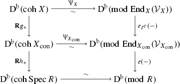
Further, under the crepant setup of 2.9, $\mathrm{End}_X(\mathcal {V}_X)\cong \mathrm{End}_R(N)$ and $\mathrm{End}_{X_{\mathrm {con}}}(\mathcal {V}_{X_{\mathrm {con}}})\cong \mathrm{End}_R(N_{I^c})$, so $\mathrm{End}_R(N_{I^c})$ is derived equivalent to $X_{\mathrm {con}}$ via the tilting bundle $\mathcal {V}_{X_{\mathrm {con}}}$.

Proof

(1) As in Sect. 2.1, by the vanishing theorem $\mathbf{R}{g}_*\mathcal {O}_X\cong \mathcal {O}_{X_{\mathrm {con}}}$. Given this, the proof of [26, 4.6] (which considered surfaces and ${}^{-1}\mathfrak {Per}$ instead) shows that $g^*(\mathcal {V}_{X_{\mathrm {con}}}^*)\cong \mathcal {O}_X\oplus _{j\notin I}\mathcal {M}_j$. Thus

$$\begin{aligned} \mathcal {H}om_X(g^*\mathcal {V}_{X_{\mathrm {con}}},\mathcal {O}_X)\cong g^*\mathcal {H}om_X(\mathcal {V}_{X_{\mathrm {con}}},\mathcal {O}_{X_{\mathrm {con}}})\cong \mathcal {O}_X\oplus _{j\notin I}\mathcal {M}_j \end{aligned}$$

and so dualizing gives $g^*\mathcal {V}_{X_{\mathrm {con}}}\cong \mathcal {O}_X\oplus _{j\notin I}\mathcal {N}_j:=\mathcal {N}_{I^c}$, where the right-hand side is a summand of $\mathcal {V}_X$. Applying $\mathbf{R}{g}_*$ and using the projection formula

$$\begin{aligned} \mathcal {V}_{X_{\mathrm {con}}}\cong \mathbf{R}{g}_*g^*\mathcal {V}_{X_{\mathrm {con}}}\cong \mathbf{R}{g}_* \mathcal {N}_{I^c} \end{aligned}$$

and so inspecting cohomology shows that $g_*\mathcal {N}_{I^c}\cong \mathbf{R}{g}_*\mathcal {N}_{I^c}\cong \mathcal {V}_{X_{\mathrm {con}}}$. It follows that

$$\begin{aligned} \mathrm{End}_{X_{\mathrm {con}}}(\mathcal {V}_{X_{\mathrm {con}}})=\mathrm{End}_{X_{\mathrm {con}}}(g_*\mathcal {N}_{I^c})\cong \mathrm{Hom}_X(g^*g_*\mathcal {N}_{I^c},\mathcal {N}_{I^c})\cong \mathrm{End}_X(\mathcal {N}_{I^c}), \end{aligned}$$

and chasing through shows this isomorphism is a ring isomorphism.

(2) The commutativity of the top diagram follows from the functorial isomorphisms

$$\begin{aligned} {\mathbf{R}\text {Hom}}_{X_{\mathrm {con}}}(\mathcal {V}_{X_{\mathrm {con}}},\mathbf{R}{g}_* (-))&\cong {\mathbf{R}\text {Hom}}_{X}(g^*\mathcal {V}_{X_{\mathrm {con}}},-)\\&\cong {\mathbf{R}\text {Hom}}_{X}(\mathcal {N}_{I^c},-)\\&\cong e_{I^c}{\mathbf{R}\text {Hom}}_{X}(\mathcal {V}_X,-). \end{aligned}$$

with the bottom diagram being similar. The last statements then follow from 2.12. $\square$

The following is an easy extension of [52, 3.2], and will be needed later to read off the dual graph after the flop.

Theorem 2.15

In the general setup of 2.8, set $\Lambda :=\mathrm{End}_X(\mathcal {V}_X)$. Then $\Lambda ^{\mathrm{op}}$ can be written as a quiver with relations, where the quiver is given as follows: for every exceptional curve $C_i$ associate a vertex labelled i, and also associate a vertex $\star$ corresponding to $\mathcal {O}_{X}$. Then the number of arrows between the vertices is precisely

	Number of arrows	If setup 2.9, $d=3$ and X is smooth
$\star \rightarrow \star$	$\dim _\mathbb {C}\mathrm{Ext}_X^1(\omega _C,\omega _C)$.
$i\rightarrow \star$	$\dim _\mathbb {C}\mathrm{Hom}_X(\mathcal {O}_{C_i}(-1),\omega _C)$
$\star \rightarrow i$	$\dim _\mathbb {C}\mathrm{Ext}_X^2(\omega _C,\mathcal {O}_{C_i}(-1))$
$i\rightarrow i$	$\dim _\mathbb {C}\mathrm{Ext}_X^1(\mathcal {O}_{C_i},\mathcal {O}_{C_i})$	$=\left\{ \begin{array}{rl} 0&{} \hbox {if }(-1,-1)\hbox {-curve}\\ 1 &{}\hbox {if }(-2,0)\hbox {-curve}\\ 2&{}\hbox {if }(-3,1)\hbox {-curve} \end{array}\right.$
$i\rightarrow j$	$\left\{ \begin{array}{rl} 1&{} \hbox {if }C_i\cap C_j=\{\mathrm {pt}\}\\ 0 &{}\hbox {else} \end{array}\right.$

where in the bottom row $i\ne j$.

2.3 Mutation

Throughout this subsection R denotes a normal d-sCY complete local commutative algebra, with $d\ge 2$, and $M\in \mathrm{ref}\,R$ denotes a basic modifying module M. We summarise and extend the theory of mutation from [23, §6] and [15, §5].

Setup 2.16

With assumptions as above, given the basic modifying R-module M, set $\Lambda :=\mathrm{End}_R(M)$ and pick a summand $M_I$ of M.

• (1) Denote $M_{I^c}$ to be the complement of $M_I$, so that

  $$\begin{aligned} M=M_I\oplus M_{I^c}. \end{aligned}$$

• (2) We define $[M_{I^c}]$ to be the two-sided ideal of $\Lambda$ consisting of morphisms $M\rightarrow M$ which factor through a member of $\mathrm{add}\,M_{I^c}$. We define $\Lambda _I:=\Lambda /[M_{I^c}]$. Equivalently, if $e_{I}$ denotes the idempotent of $\Lambda =\mathrm{End}_R(M)$ corresponding to the summand $M_{I}$ of M, then $\Lambda _I=\Lambda /\Lambda (1-e_{I})\Lambda$.

Given our choice of summand $M_I$, we then mutate. In the theory of mutation, the complement submodule $M_{I^c}$ is fixed, and the summand $M_I$ changes in a universal way. Recall from Sect. 2.1 that $(-)^*:=\mathrm{Hom}_R(-,R)$.

Setup 2.17

With the setup as in 2.16, write $M_I=\bigoplus _{i\in I}M_i$ as a direct sum of indecomposables. For each $i\in I$, consider a minimal right $(\mathrm{add}\,M_{I^c})$-approximation

$$\begin{aligned} V_i\xrightarrow {a_i}M_i \end{aligned}$$

of $M_i$, which by definition means that

• (1) $V_i\in \mathrm{add}\,M_{I^c}$ and $(\cdot a_i):\mathrm{Hom}_R(M_{I^c},V_i)\rightarrow \mathrm{Hom}_R(M_{I^c},M_i)$ is surjective,

• (2) If $g\in \mathrm{End}_R(V_i)$ satisfies $a_i=ga_i$, then g is an automorphism.

Since R is complete, such an $a_i$ exists and is unique up to isomorphism. Denote $K_i:=\mathrm{Ker}\,a_i$, so there is an exact sequence

$$\begin{aligned} 0\rightarrow K_i\xrightarrow {c_i} V_i\xrightarrow {a_i}M_i \end{aligned}$$

(2.C)

such that

$$\begin{aligned} 0\rightarrow \mathrm{Hom}_R(M_{I^c},K_i)\xrightarrow {\cdot c_i} \mathrm{Hom}_R(M_{I^c},V_i)\xrightarrow {\cdot a_i}\mathrm{Hom}_R(M_{I^c},M_i)\rightarrow 0\nonumber \\ \end{aligned}$$

(2.D)

is exact. Summing the sequences (2.C) over all $i\in I$ gives an exact sequence

$$\begin{aligned} 0\rightarrow K_I\xrightarrow {c} V_I\xrightarrow {a}M_I \end{aligned}$$

(2.E)

such that

$$\begin{aligned} 0\rightarrow \mathrm{Hom}_R(M_{I^c},K_I)\xrightarrow {\cdot c} \mathrm{Hom}_R(M_{I^c},V_I)\xrightarrow {\cdot a}\mathrm{Hom}_R(M_{I^c},M_I)\rightarrow 0\nonumber \\ \end{aligned}$$

(2.F)

is exact.

Dually, for each $i\in I$, consider a minimal right $(\mathrm{add}\,M_{I^c}^*)$-approximation

$$\begin{aligned} U_i^*\xrightarrow {b_i}M_i^* \end{aligned}$$

of $M_i^*$, and denote $J_i:=\mathrm{Ker}\,b_i$. Thus

$$\begin{aligned}&0\rightarrow J_i\xrightarrow {d_i} U_i^*\xrightarrow {b_i}M_i^* \end{aligned}$$

(2.G)

$$\begin{aligned}&0\rightarrow \mathrm{Hom}_R(M_{I^c}^*,J_i)\xrightarrow {\cdot d_i} \mathrm{Hom}_R(M_{I^c}^*,U_i^*)\xrightarrow {\cdot b_i} \mathrm{Hom}_R(M_{I^c}^*,M_i^*) \rightarrow 0 \nonumber \\ \end{aligned}$$

(2.H)

are exact. Summing over all $i\in I$ gives exact sequences

$$\begin{aligned}&0\rightarrow J_I\xrightarrow {d} U_I^*\xrightarrow {b}M_I^* \end{aligned}$$

(2.I)

$$\begin{aligned}&0\rightarrow \mathrm{Hom}_R(M_{I^c}^*,J_I)\xrightarrow {\cdot d} \mathrm{Hom}_R(M_{I^c}^*,U_I^*)\xrightarrow {\cdot b} \mathrm{Hom}_R(M_{I^c}^*,M_I^*) \rightarrow 0. \nonumber \\ \end{aligned}$$

(2.J)

Definition 2.18

With notation as above,

• (1) We define the right mutation of M at $M_I$ as

  $$\begin{aligned} \upmu _{I}M:=M_{I^c}\oplus K_I, \end{aligned}$$

  that is we remove the summand $M_I$ and replace it with $K_I$.

• (2) We define the left mutation of M at $M_I$ as

  $$\begin{aligned} \upnu _{I}M:=M_{I^c}\oplus (J_I)^*. \end{aligned}$$

In this level of generality, $\upnu _IM$ is not necessarily isomorphic to $\upmu _IM$.

Remark 2.19

Even if $M_I=M_i$ is indecomposable, when we view $\mathrm{End}_R(M)$ as a quiver with relations, with arrows a, and left projective $\mathrm{End}_R(M)$-modules $P_j$ corresponding to the indecomposable summands $M_j$, it is a common misconception that mutation can be defined using simply the arrows into (respectively, out of) the vertex i. Indeed, we could consider the combinatorially defined morphisms

$$\begin{aligned} \bigoplus _{\begin{array}{c} \mathrm {head}(a)=i\\ \mathrm {tail}(a)\ne i \end{array}}P_{\mathrm {tail}(a)}\rightarrow P_i\quad \hbox {and}\quad P_i\rightarrow \bigoplus _{\begin{array}{c} \mathrm {tail}(a)=i\\ \mathrm {head}(a)\ne i \end{array}}P_{\mathrm {head}(a)} \end{aligned}$$

which by reflexive equivalence arise from morphisms

$$\begin{aligned} \bigoplus _{\begin{array}{c} \mathrm {head}(a)=i\\ \mathrm {tail}(a)\ne i \end{array}}M_{\mathrm {tail}(a)}\rightarrow M_i\quad \hbox {and}\quad M_i\rightarrow \bigoplus _{\begin{array}{c} \mathrm {tail}(a)=i\\ \mathrm {head}(a)\ne i \end{array}}M_{\mathrm {head}(a)}. \end{aligned}$$

However these morphisms are not approximations in general. In other words, the mutation defined in 2.18 above is not in general a vertex tilt in the sense of Bridgeland–Stern [6], and in full generality there is no simple combinatorial description of the decomposition of $U_I$ or $V_I$. In the case of cDV singularities, we do give a combinatorial description later in Sects. 5.3 and 5.4 by relating the problem to partial crepant resolutions of ADE singularities.

One of the key properties of mutation is that it always gives rise to a derived equivalence. With the setup as above, for the case of left mutation $\upnu _{I}M$, the derived equivalence between $\mathrm{End}_R(M)$ and $\mathrm{End}_R(\upnu _{I}M)$ is given by a tilting $\mathrm{End}_R(M)$-module $T_I$ constructed as follows. By (A.C) there is an exact sequence

$$\begin{aligned} 0\rightarrow M_I\xrightarrow {b^*} U_I\rightarrow J_I^* \end{aligned}$$

obtained by dualizing (2.I). Applying $\mathrm{Hom}_R(M,-)$ induces $(\cdot b^* ):\mathrm{Hom}_R(M,M_I)\rightarrow \mathrm{Hom}_R(M,U_I)$, so denoting the cokernel by $C_I$ we obtain an exact sequence

$$\begin{aligned} 0\rightarrow \mathrm{Hom}_R(M,M_I)\xrightarrow {\cdot b^*} \mathrm{Hom}_R(M,U_I)\rightarrow C_I\rightarrow 0. \end{aligned}$$

(2.K)

The tilting $\mathrm{End}_R(M)$-module $T_I$ is defined to be $T_I:=\mathrm{Hom}_R(M,M_{I^c})\oplus C_I$. It turns out that $\mathrm{End}_\Lambda (T_I)\cong \mathrm{End}_R(\upnu _IM)$ [23, 6.7, 6.8], and there is always an equivalence

$$\begin{aligned} \Phi _I:={\mathbf{R}\text {Hom}}(T_I,-):\mathrm{{D}^b}(\hbox {mod}\,\mathrm{End}_{R}(M))\rightarrow \mathrm{{D}^b}(\hbox {mod}\,\mathrm{End}_{R}(\upnu _{I}M)), \end{aligned}$$

(2.L)

which is called the mutation functor [23, 6.8]. It is never the identity functor. On the other hand $\upnu _{I}M=M$ can happen (see e.g. A.2). Note that, by construction, $T_I$ has the structure of a $\Lambda$-$\Gamma$ bimodule, where $\Gamma :=\upnu _I\Lambda :=\mathrm{End}_\Lambda (T_I)\cong \mathrm{End}_R(\upnu _IM)$. The following is elementary.

Lemma 2.20

With notation as above, the following statements hold.

• (1) $T_I$ is a tilting $\Lambda$-module with $\mathrm {pd}_\Lambda T_I=1$.

• (2) $T_I$ is a tilting $\Gamma ^{\mathrm{op}}\cong \mathrm{End}_R((\upnu _IM)^*)$-module, with $T_I\cong \mathrm{Hom}_R((\upnu _IM)^*, M_{I^c}^*)\oplus D_I$ where $D_I$ arises from the exact sequence

  $$\begin{aligned} 0\rightarrow \mathrm{Hom}_R((\upnu _IM)^*,J_I)\xrightarrow {\cdot d}\mathrm{Hom}_R((\upnu _IM)^*,U_I^*)\rightarrow D_I\rightarrow 0 \end{aligned}$$

  of $\Gamma ^{\mathrm{op}}$-modules. Thus $\mathrm {pd}_{\Gamma ^{\mathrm{op}}}T_I=1$ and $\mathrm{End}_{\Gamma ^{\mathrm{op}}}(T_I)\cong \Lambda ^{\mathrm{op}}$.

Proof

(1) is [23, 6.8], and (2) follows from (1), see for example [45, 2.2] or [31, 4.1], [4, 2.6]. As a sketch proof, by (2.K)

$$\begin{aligned} 0\rightarrow \mathrm{Hom}_R(M,M)\rightarrow \mathrm{Hom}_R(M,U_I\oplus M_{I^c})\rightarrow C_I\rightarrow 0. \end{aligned}$$

is exact, and applying $\mathrm{Hom}_\Lambda (-,T_I)$ gives an exact sequence

$$\begin{aligned} 0\rightarrow \mathrm{Hom}_\Lambda (C_I,T_I)\rightarrow \mathrm{Hom}_\Lambda (\mathrm{Hom}_R(M,U_I\oplus M_{I^c}),T_I)\rightarrow T_I\rightarrow 0\nonumber \\ \end{aligned}$$

(2.M)

of $\Gamma ^{\mathrm{op}}$-modules. Under the isomorphism $\mathrm{End}_\Lambda (T_I)\cong \mathrm{End}_R(\upnu _IM)$,

$$\begin{aligned} \mathrm{Hom}_\Lambda (C_I,T_I)&\cong \mathrm{Hom}_R(J_I^*,\upnu _IM)\cong \mathrm{Hom}_R((\upnu _IM)^*,J_I),\\ \mathrm{Hom}_\Lambda (\mathrm{Hom}_R(M,U_I\oplus M_{I^c}),T_I)&\cong \mathrm{Hom}_R(U_I\oplus M_{I^c},\upnu _IM)\\&\cong \mathrm{Hom}_R((\upnu _IM)^*,U_I^*\oplus M_{I^c}^*), \end{aligned}$$

so (2.M) is isomorphic to

$$\begin{aligned} 0\rightarrow \mathrm{Hom}_R((\upnu _IM)^*,J_I)\xrightarrow {{\cdot d\atopwithdelims ()0}}\mathrm{Hom}_R((\upnu _IM)^*,U_I^*\oplus M_{I^c}^*)\rightarrow T_I\rightarrow 0, \end{aligned}$$

proving the statements by applying the analysis in (1) to $\mathrm{End}_R((\upnu _IM)^*)$. $\square$

For our purposes later we will require the finer information encoded in the following two key technical results. They are both an extension of [23, §6] and [15, §4], and are proved using similar techniques, so we postpone the proofs until “Appendix A”.

Theorem 2.21

($=$ A.5) Suppose that $\upnu _I M\cong M$. Then

• (1) $T_I=\Lambda (1-e_I)\Lambda$ and $\Gamma :=\mathrm{End}_\Lambda (T_I)\cong \Lambda$.

• (2) $\Omega _\Lambda \Lambda _I=T_I$, thus $\mathrm {pd}_\Lambda \Lambda _I=2$ and $\mathrm{Ext}^1_\Lambda (T_I,-)\cong \mathrm{Ext}^2_\Lambda (\Lambda _I,-)$.

Theorem 2.22

($=$ A.8) Suppose that $d= 3$, $\upnu _I \upnu _IM\cong M$ and $\dim _{\mathbb {C}}\Lambda _I<\infty$. As above, set $\Gamma :=\mathrm{End}_\Lambda (T_I)\cong \mathrm{End}_R(\upnu _IM)$. Then

• (1) $T_I\cong \mathrm{Hom}_R(M,\upnu _IM)$.

• (2) $\Omega _\Lambda ^2\Lambda _I=T_I$, thus $\mathrm {pd}_\Lambda \Lambda _I=3$ and $\mathrm{Ext}^1_\Lambda (T_I,-)\cong \mathrm{Ext}^3_\Lambda (\Lambda _I,-)$.

The following, one of the main results in [23], will allow us to establish properties non-explicitly when we restrict to minimal models and mutate at single curves.

Theorem 2.23

Suppose that $d=3$, and M is a maximal modifying R-module with indecomposable summand $M_j$. Set $\Lambda :=\mathrm{End}_R(M)$. Then

• (1) We have $\upmu _{j}(M)\cong \upnu _{j}(M)$.

• (2) Always $\upnu _j\upnu _j(M)\cong M$.

• (3) $\upnu _j(M)\ncong M$ if and only if $\dim _\mathbb {C}\Lambda _j<\infty$.

• (4) $\upnu _j(M)\cong M$ if and only if $\dim _\mathbb {C}\Lambda _j=\infty$.

Proof

(1) and (2) are special cases of [23, 6.25].

(3)($\Rightarrow$) is [23, 6.25(2)], and (4)($\Rightarrow$) is [23, 6.25(1)]. (3)($\Leftarrow$) is the contrapositive of (4)($\Rightarrow$), and (4)($\Leftarrow$) is the contrapositive of (3)($\Rightarrow$). $\square$

Remark 2.24

Theorem 2.23(3)(4) shows that there is a dichotomy in the theory of mutation depending on whether the dimension of $\Lambda _j$ is finite or not. In the flops setting, this dichotomy will correspond to the fact that in a 3-fold, an irreducible curve may or may not be floppable. In either case we will obtain a derived equivalence from mutation, and the results 2.21 and 2.22 will allow us to control it.

The above 2.23 will allow us to easily relate flops and mutations in the case when $d=3$ and the singularities of X are $\mathbb {Q}$-factorial. When we want to drop the $\mathbb {Q}$-factorial assumption, or consider $d=2$ with canonical singularities, we will need the following.

Proposition 2.25

With the crepant setup of 2.9, and notation from 2.13, choose a subset $\bigcup _{i\in I}C_i$ of curves above the origin and contract them to obtain $X\rightarrow X_{\mathrm {con}}\rightarrow \mathrm{Spec}\,R$. If $X_{\mathrm {con}}$ has only isolated hypersurface singularities, then $\upnu _I\upnu _IN\cong N$ in such a way that $N_i$ mutates to $J_i^*$ mutates to $N_i$.

Proof

Denote $\mathbb {F}:=\mathrm{Hom}_R(N_{I^c}^*,-)$. The choice of curves gives us a summand $N_I$ such that $N_{I^c}$ is a generator. This being the case, the right-hand morphisms in all the exchange sequences are all surjective. By (2.H)

$$\begin{aligned} 0\rightarrow \mathbb {F}J_i\rightarrow \mathbb {F}U^*_i\rightarrow \mathbb {F}N_i^*\rightarrow 0 \end{aligned}$$

is exact. Denoting $\Delta :=\mathrm{End}_R(N^*_{I^c})$, since $\mathbb {F}U^*_i$ is a projective $\Delta$-module, this shows that $\Omega _\Delta (\mathbb {F}N_i^*)\cong \mathbb {F}J_i$. If we denote the minimal $\mathrm{add}\,N_{I^c}^*$-approximation of $J_i$ by

$$\begin{aligned} 0\rightarrow L_i\rightarrow W_i\rightarrow J_i\rightarrow 0, \end{aligned}$$

then $\upnu _I\upnu _I$ takes $N_i$ to $J_i^*$ to $L_i^*$. We claim that $L_i^*\cong N_i$, so by reflexive equivalence it suffices to prove that $\mathbb {F}L_i\cong \mathbb {F}N_i^*$. Since

$$\begin{aligned} 0\rightarrow \mathbb {F}L_i\rightarrow \mathbb {F}W_i\rightarrow \mathbb {F}J_i\rightarrow 0 \end{aligned}$$

is exact and $\mathbb {F}W_i$ is a projective $\Delta$-module, $\Omega _\Delta (\mathbb {F}J_i)\cong \mathbb {F}L_i$, so the result follows if we can establish that $\Omega _\Delta ^2(\mathbb {F}N_i^*)\cong \mathbb {F}N_i^*$. Since $\mathbb {F}N_i^*\in \mathrm{CM}\,\Delta$ has no $\Delta$-projective summands, and $\Omega _\Delta =[-1]$ on the category ${\underline{\mathrm{CM}}}\,\Delta$, it suffices to show that $[2]=\mathrm{{Id}}$ on ${\underline{\mathrm{CM}}}\,\Delta$.

But by 2.14 $\Delta$ is derived equivalent to $X_{\mathrm {con}}$ and so

$$\begin{aligned} {\underline{\mathrm{CM}}}\,\Delta \simeq \mathrm{{D}_\mathsf{sg}}(\Delta )\simeq \mathrm{{D}_\mathsf{sg}}(X_{\mathrm {con}})\simeq \bigoplus _{x\in \mathrm{Sing}\,X_{\mathrm {con}}}{\underline{\mathrm{CM}}}\,\widehat{\mathcal {O}}_{X_{\mathrm {con}},x} \end{aligned}$$

by Orlov [40], since all categories under consideration are idempotent complete. Since each of $\widehat{\mathcal {O}}_{X_{\mathrm {con}},x}$ are hypersurfaces, $[2]=\mathrm{{Id}}$ for each of the categories on the right-hand side, so since the above are triangle equivalences, $[2]=\mathrm{{Id}}$ for the left-hand category. $\square$

In the study of terminal (and even smooth) 3-folds, canonical surfaces appear naturally via hyperplane sections, and in this setting $\mathrm {pd}_\Lambda \Lambda _i$ can be infinite, which is very different to 2.21 and 2.22. The next result will allow us to bypass this problem.

Proposition 2.26

Suppose that R is a normal complete local 2-sCY commutative algebra, and $M\in \mathrm{CM}\,R$ is basic. Choose a summand $M_I$, set $\Lambda :=\mathrm{End}_R(M)$ and denote the simple $\Lambda$-modules by $S_j$. Assume that $\upnu _I\upnu _IM\cong M$. If $x\in \mathrm{fdmod}\,\Lambda$ with $\mathrm{Hom}_\Lambda (x,S_i)=0$ for all $i\in I$, then $\mathrm{Ext}^1_\Lambda (T_I,x)=0$.

Proof

Since $\Lambda$ is 2-sCY, x has finite length and $C_I$ has finite projective dimension,

$$\begin{aligned} \mathrm{Ext}^1_\Lambda (T_I,x)\cong \mathrm{Ext}^1_\Lambda (C_I,x)\cong D\mathrm{Ext}^1_\Lambda (x,C_I), \end{aligned}$$

so it suffices to show that $\mathrm{Ext}^1_\Lambda (x,C_I)=0$. By the assumption $\upnu _I\upnu _IM\cong M$, it follows that $J_I^*\cong K_I$. Since $0\rightarrow \mathrm{Hom}_R(M,M_I)\rightarrow \mathrm{Hom}_R(M,U_I)\rightarrow \mathrm{Hom}_R(M,K_I)$ is exact, splicing we obtain exact sequences

$$\begin{aligned}&0\rightarrow \mathrm{Hom}_R(M,M_I)\rightarrow \mathrm{Hom}_R(M,U_I)\rightarrow C_I\rightarrow 0 \end{aligned}$$

(2.N)

$$\begin{aligned}&0\rightarrow C_I\rightarrow \mathrm{Hom}_R(M,K_I)\rightarrow F_I\rightarrow 0 \end{aligned}$$

(2.O)

But by (A.E)

$$\begin{aligned} 0\rightarrow \mathrm{Hom}_R(M_{I^c},M_I)\rightarrow \mathrm{Hom}_R(M_{I^c},U_I)\rightarrow \mathrm{Hom}_R(M_{I^c},K_I)\rightarrow 0 \end{aligned}$$

is exact, so $F_I$ is a finitely generated $\Lambda _I$-module. But since $d=2$ and R is normal, necessarily $\Lambda _I$ has finite length, hence so too has $F_I$. Thus the assumptions then imply that $\mathrm{Hom}_\Lambda (x,F_I)=0$, so $\mathrm{Ext}^1_\Lambda (x,C_I)\hookrightarrow \mathrm{Ext}^1_\Lambda (x,\mathrm{Hom}_R(M,K_I))$.

Hence it suffices to show that $\mathrm{Ext}^1_\Lambda (x,\mathrm{Hom}_R(M,K_I))=0$. But

$$\begin{aligned} 0\rightarrow \mathrm{Hom}_R(M,K_I)\xrightarrow {\cdot c} \mathrm{Hom}_R(M,V_I)\rightarrow \mathrm{Hom}_R(M,M_I)\rightarrow \Lambda _I\rightarrow 0 \end{aligned}$$

is exact, so denoting $E_I:=\mathrm{Cok}(\cdot c)$, then $\mathrm{Hom}_\Lambda (x,E_I)$ embeds inside

$$\begin{aligned} \mathrm{Hom}_\Lambda (x,\mathrm{Hom}_R(M,M_I))\cong D\,\mathrm{Ext}^2_\Lambda (\mathrm{Hom}_R(M,M_I),x)=0, \end{aligned}$$

so $\mathrm{Hom}_\Lambda (x,E_I)=0$. This in turns implies that $\mathrm{Ext}^1_\Lambda (x,\mathrm{Hom}_R(M,K_I))$ embeds inside $\mathrm{Ext}^1_\Lambda (x,\mathrm{Hom}_R(M,V_I))$, which is zero. Thus $\mathrm{Ext}^1_\Lambda (x,\mathrm{Hom}_R(M,K_I))=0$, as required. $\square$

3 Contractions and deformation theory

The purpose of this section is use noncommutative deformations to detect whether a divisor has been contracted to a curve, in such a manner that is useful for iterations, improving [16]. This part of the Homological MMP does not need any restriction on singularities, so throughout this section we adopt the general setup of 2.8.

3.1 Background on noncommutative deformations

With the setup $f:X\rightarrow \mathrm{Spec}\,R$ of 2.8, set $\Lambda :=\mathrm{End}_X(\mathcal {V}_X)$. Given any $E\in \mathrm{coh}\,X$, there is an associated classical commutative deformation functor

$$\begin{aligned} c\mathcal {D}ef_E:\mathsf {cart}_1\rightarrow \mathsf {Sets}\end{aligned}$$

where $\mathsf {cart}_1$ denotes the category of local commutative artinian $\mathbb {C}$-algebras. The definition of this functor, which we do not state here, involves a flatness condition over the test object $R\in \mathsf {cart}_1$.

Noncommutative deformations add two new features to this classical picture. First, the test objects are enlarged from commutative artinian rings to allow certain (basic) noncommutative artinian $\mathbb {C}$-algebras. This thickens the universal sheaf. Second, they allow us to deform a finite collection $\{E_i\mid i\in I\}$ of objects whilst remembering Ext information between them.

For the purposes of this paper, we will not deform coherent sheaves, but rather their images under the derived equivalence in Sect. 2.2. Deforming on either side of the derived equivalence turns out to give the same answer [16], but the noncommutative side is slightly easier to formulate. Thus we input a finite collection $\{S_i\mid i\in I\}$ of simple $\Lambda$-modules, and define the associated noncommutative deformation functor as follows.

As preparation, recall that an n-pointed $\mathbb {C}$-algebra $\Gamma$ is an associative $\mathbb {C}$-algebra, together with $\mathbb {C}$-algebra morphisms $p:\Gamma \rightarrow \mathbb {C}^n$ and $i:\mathbb {C}^n \rightarrow \Gamma$ such that $i p = \mathrm{{Id}}$. A morphism of n-pointed $\mathbb {C}$-algebras $\uppsi :(\Gamma ,p,i)\rightarrow (\Gamma ',p',i')$ is a ring homomorphism $\uppsi :\Gamma \rightarrow \Gamma '$ such that

commutes. We denote the category of n-pointed $\mathbb {C}$-algebras by $\mathsf {Alg}_n$, and denote the full subcategory consisting of those objects that are commutative rings by $\mathsf {CAlg}_n$. Furthermore, denote by $\mathsf {art}_n$ the full subcategory of $\mathsf {Alg}_n$ consisting of objects $(\Gamma ,p,i)$ for which $\dim _{\mathbb {C}}\Gamma <\infty$ and the augmentation ideal $\mathfrak {n}:=\mathrm{Ker}\,(p)$ is nilpotent. The full subcategory of $\mathsf {art}_n$ consisting of those objects that are commutative rings is denoted $\mathsf {cart}_n$.

Given $\Gamma \in \mathsf {art}_n$, the morphism i produces n idempotents $e_1,\ldots ,e_n\in \Gamma$, and we denote $\Gamma _{ij}:=e_i\Gamma e_j$.

Definition 3.1

[37] Fix a finite collection $\mathcal {S}:=\{S_i\mid i\in I\}$ of left $\Lambda$-modules. Then

• (1) For $\Gamma \in \mathsf {art}_{|I|}$, we say that $M\in \mathrm{Mod}\,\Lambda \otimes _{\mathbb {C}}\Gamma ^{\mathrm{op}}$ (i.e. a $\Lambda$-$\Gamma$ bimodule) is $\Gamma$-matric-free if

  $$\begin{aligned} M \cong (S_i\otimes _{\mathbb {C}} \Gamma _{ij}) \end{aligned}$$

  as $\Gamma ^{\mathrm{op}}$-modules, where the right-hand side is the matrix built by varying $i,j\in \{1,\ldots ,n\}$, which has an obvious $\Gamma ^{\mathrm{op}}$-module structure.

• (2) The noncommutative deformation functor

  $$\begin{aligned} \mathcal {D}ef_{\mathcal {S}}:\mathsf {art}_n\rightarrow \mathsf {Sets}\end{aligned}$$

  is defined by sending

  $$\begin{aligned} (\Gamma ,\mathfrak {n})\mapsto \left. \left\{ (M,\delta ) \left| \begin{array}{l}M\in \mathrm{Mod}\,\Lambda \otimes _{\mathbb {C}}\Gamma ^{\mathrm{op}}\\ M \text { is }\Gamma \text {-matric-free}\\ \delta =(\delta _i)\hbox { with }\delta _i:M\otimes _\Gamma (\Gamma /\mathfrak {n})e_i\xrightarrow {\sim } S_i \end{array}\right. \right\} \bigg / \sim \right. \end{aligned}$$

  where $(M,\delta )\sim (M',\delta ')$ if there exists an isomorphism $\tau :M\rightarrow M'$ of bimodules such that

  

  commutes, for all i.

• (3) The commutative deformation functor is defined to be the restriction of $\mathcal {D}ef_{\mathcal {S}}$ to $\mathsf {cart}_{|I|}$, and is denoted $c\mathcal {D}ef_{\mathcal {S}}$.

Given the general setup $f:X\rightarrow \mathrm{Spec}\,R$ of 2.8, choose a subset of curves $\bigcup _{i\in I}C_i$ above the unique closed point and contract them as in Sect. 2.1 to factorise f as

$$\begin{aligned} X\xrightarrow {g}X_{\mathrm {con}}\xrightarrow {h}\mathrm{Spec}\,R \end{aligned}$$

with $\mathbf{R}{g}_*\mathcal {O}_X=\mathcal {O}_{X_{\mathrm {con}}}$ and $\mathbf{R}{h}_*\mathcal {O}_{X_{\mathrm {con}}}=\mathcal {O}_{R}$. By 2.11, across the derived equivalence the coherent sheaves $\mathcal {O}_{C_i}(-1)\in \mathrm{coh}\,X$ ($i\in I$) correspond to simple left $\Lambda$-modules $S_i$. The following is the $d=3$ special case of the main result of [16].

Theorem 3.2

(Contraction theorem) With the general setup in 2.8, if $d=3$ then f contracts $\bigcup _{i\in I}C_i$ to a point without contracting a divisor if and only if $\mathcal {D}ef_{\mathcal {S}}$ is representable.

3.2 Global and local contraction algebras

We maintain the notation from the general setup of the previous subsection. In this subsection we detect whether g contracts a curve without contracting a divisor by using the algebra $\Lambda =\mathrm{End}_X(\mathcal {V}_X)$, constructed in Sect. 2.2 using the morphism f. This will allow us to iterate.

Definition 3.3

For $\Lambda =\mathrm{End}_X(\mathcal {V}_X)$, with notation from 2.13 define $[\mathcal {N}_{I^c}]$ to be the 2-sided ideal of $\Lambda$ consisting of morphisms that factor through $\mathrm{add}\,\mathcal {N}_{I^c}$, and set $\Lambda _I:=\Lambda /[\mathcal {N}_{I^c}]$.

In [16] the prorepresenting object of $\mathcal {D}ef_{\mathcal {S}}$ was constructed locally with respect to the morphism g, using the following method. Let $x\in X_{\mathrm {con}}$ be the closed point above which sits $\bigcup _{i\in I}C_i$. Choose an affine neighbourhood $U_{\mathrm {con}}:=\mathrm{Spec}\,R'$ containing x, set $U:=g^{-1}(U_{\mathrm {con}})$, let $\mathfrak {R}'$ be the completion of $R'$ at x, and consider the formal fibre $\mathfrak {U}\rightarrow \mathrm{Spec}\,\mathfrak {R}'$. This morphism satisfies all the assumptions of the general setup of 2.8, and we define the contraction algebra to be $\mathrm {A}_{\mathrm {con}}^I:=\mathrm{End}_{\mathfrak {U}}(\mathcal {V}_{\mathfrak {U}})/[\mathcal {O}_{\mathfrak {U}}]$. By [15, 16] the contraction algebra is independent of choice of U, and

$$\begin{aligned} \mathcal {D}ef_{\mathcal {S}}(-)\cong \mathrm{Hom}_{\mathsf {Alg}_{|I|}}(\mathrm {A}_{\mathrm {con}}^{I},-). \end{aligned}$$

(3.A)

Even in the case $|I|=1$, comparing $\Lambda _I$ and $\mathrm {A}_{\mathrm {con}}^I$ directly is a subtle problem. If $|I|=1$ and the scheme-theoretic multiplicity of $C_i$ with respect to g is n, then we can view $\mathrm {A}_{\mathrm {con}}^{\{i\}}$ as factor of an endomorphism ring of an indecomposable rank n bundle on $\mathfrak {U}$. On the other hand, $\Lambda _i$ can be viewed as a factor of an endomorphism ring of an indecomposable rank m bundle on X, where m is the scheme theoretic multiplicity of $C_i$ with respect to the morphism f. The next example demonstrates that $m\ne n$ in general.

Example 3.4

Consider the $cD_4$ singularity $R:=\mathbb {C}[[u,x,y,z]]/(u^2-xyz)$, which is isomorphic to the toric quotient singularity $\mathbb {C}^3/G$ where $G=\mathbb {Z}_2\times \mathbb {Z}_2\le \mathrm{SL}(3,\mathbb {C})$. We consider $X^+=G\mathrm {-Hilb}(\mathbb {C}^3)$, and one of its flops

Locally, being the Atiyah flop, the scheme theoretic multiplicity of the flopping curve with respect to g is one, but with respect to f the scheme theoretic multiplicity is two. This can be calculated directly, but it also follows from the example 7.6 later, once we have proved 4.6.

The following is the main result of this section.

Theorem 3.5

With the general setup in 2.8, suppose that $d=3$ and pick a subset $\bigcup _{i\in I}C_i$ of curves above the origin. Then

• (1) $\mathcal {D}ef_{\mathcal {S}}\cong \mathrm{Hom}_{\mathsf {Alg}_{|I|}}(\Lambda _I,-)$.

• (2) $\Lambda _I\cong \mathrm {A}_{\mathrm {con}}^I$.

• (3) $\bigcup _{i\in I}C_i$ contracts to point without contracting a divisor $\Leftrightarrow \dim _{\mathbb {C}}\Lambda _I<\infty$.

Proof

(1) Arguing exactly as in [15, 3.1], since $S_i=\mathbb {C}$ as $\Lambda$-modules, if we denote the natural homomorphisms $\Lambda \rightarrow S_i$ by $q_i$, then for $(\Gamma ,\mathfrak {n})\in \mathsf {art}_{|I|}$,

$$\begin{aligned} \mathcal {D}ef_{\mathcal {S}}(\Gamma )&\cong \left. \left\{ \begin{array}{cl} \bullet &{} \hbox {A left } \Lambda \hbox {-module structure on }(S_i\otimes _{\mathbb {C}}\Gamma _{ij}) \hbox { such that}\\ &{}(S_i\otimes _{\mathbb {C}}\Gamma _{ij})\hbox { becomes a } \Lambda \hbox {-}\Gamma \hbox { bimodule.}\\ \bullet &{} \delta =(\delta _i)\hbox { such that } \delta _i:(S_i\otimes _{\mathbb {C}}\Gamma _{ij})\otimes _\Gamma (\Gamma /\mathfrak {n})e_i \xrightarrow {\sim }S_i\\ &{}\hbox { as }\Lambda \hbox {-modules} \end{array} \right\} \bigg / \sim \right. \\&\cong \left. \left\{ \begin{array}{l} \hbox {A }\mathbb {C}\hbox {-algebra homomorphism }\Lambda \rightarrow \Gamma \hbox { such that the}\\ \hbox {composition }\Lambda \rightarrow \Gamma \rightarrow (\Gamma /\mathfrak {n})e_i=S_i\hbox { is }q_i \hbox { for all }i\in I\end{array} \right\} \bigg / \sim \right. \\&\cong \mathrm{Hom}_{\mathsf {Alg}_{|I|}}(\Lambda _I,\Gamma ). \end{aligned}$$

(2) Since R is complete, both $\mathrm {A}_{\mathrm {con}}^I$ and $\Lambda _I$ belong to the pro-category of $\mathsf {art}_{|I|}$, so $\mathcal {D}ef_{\mathcal {S}}$ is prorepresented by both $\Lambda _I$ and $\mathrm {A}_{\mathrm {con}}^I$. Hence by uniqueness of prorepresenting object, $\mathrm {A}_{\mathrm {con}}^I\cong \Lambda _I$.

(3) This follows by combining (1) and 3.2. $\square$

4 Mutation, flops and twists

4.1 Flops and mutation

We now consider the crepant setup of 2.9 with $d=3$, namely $f:X\rightarrow \mathrm{Spec}\,R$ is a crepant projective birational morphism, with one dimensional fibres, where R is a complete local Gorenstein algebra, and X has at worst Gorenstein terminal singularities. As in Sect. 2.2, we consider $\mathcal {V}_X$, the basic progenerator of ${}^{0}\mathfrak {Per}(X,R)$, set $N:=H^0(\mathcal {V}_X)$ and by 2.12 denote $\Lambda :=\mathrm{End}_X(\mathcal {V}_X)\cong \mathrm{End}_R(N)$.

Remark 4.1

It also follows from 2.12 that $\mathrm{End}_X(\mathcal {V}_X)/[\mathcal {N}_{I^c}]\cong \mathrm{End}_R(N)/[N_{I^c}]$ and so the $\Lambda _I$ defined in 3.3 and 2.16 coincide. This allows us to link the previous contraction section to mutation.

We aim to prove the following theorem.

Theorem 4.2

With the crepant setup as above, with $d=3$, pick a subset of curves $\bigcup _{i\in I}C_i$ above the origin, and suppose that $\dim _{\mathbb {C}}\Lambda _I<\infty$ (equivalently, by 3.5, the curves flop). Denote the flop by $X^+$, then

• (1) $\upnu _IN\cong H^0(\mathcal {V}_{X^+})$, where $\mathcal {V}_{X^+}$ is the basic progenerator of ${}^{0}\mathfrak {Per}(X^+,R)$.

• (2) The following diagram of equivalences is naturally commutative

  

  where $\mathsf{{Flop}}$ is the inverse of the Bridgeland–Chen flop functor, $\Psi _X$ and $\Psi _{X^+}$ are the tilting equivalences in (1.A), and $\Phi _I$ is the mutation functor in (2.L).

The proof of 4.2 will be split into two stages. Stage one, proved in this subsection, is to establish 4.2(1) in the case where X is a minimal model and $I=\{i \}$. Stage two is then to prove 4.2 in full generality, lifting the $\mathbb {Q}$-factorial and $|I|=1$ assumption. The second stage uses the Auslander–McKay correspondence in Sect. 4.2, together with the Bongartz completion to pass to the minimal model, before we then contract back down. Thus, the full proof of 4.2 will not finally appear until Sect. 4.3.

To establish functoriality, the following results will be useful later.

Proposition 4.3

Suppose that $f:X\rightarrow \mathrm{Spec}\,R$ and $f':X'\rightarrow \mathrm{Spec}\,R$ both satisfy the crepant setup 2.9, and admit a common contraction

Suppose that g and $g'$ contract the same number of curves, and denote the contracted curves by $\{C_i\mid i\in I\}$ and $\{C'_i\mid i\in I\}$ respectively. If $\Theta :\mathrm{{D}^b}(\mathrm{coh}\,X)\rightarrow \mathrm{{D}^b}(\mathrm{coh}\,X')$ is a Fourier–Mukai equivalence that satisfies

• (1) $\mathbf{R}{g}'_*\circ \Theta \cong \mathbf{R}{g}_*$

• (2) $\Theta (\mathcal {O}_X)\cong \mathcal {O}_{X'}$

• (3) $\Theta (\mathcal {O}_{C_i}(-1))\cong \mathcal {O}_{C'_i}(-1)$ for all $i\in I$,

then $\Theta \cong \upphi _*$ where $\upphi :X\rightarrow X'$ is an isomorphism such that $g'\circ \upphi =g$,

Proof

This is identical to [15, §7.6], which itself is based on [46]. As in [15, 7.17], from properties (1) and (3) it follows that $\Theta$ takes ${}^{0}\mathfrak {Per}(X,X_{\mathrm {con}})$ to ${}^{0}\mathfrak {Per}(X',X_{\mathrm {con}})$. The argument is then word-for-word identical to the proof of [15, 7.17, 7.18], since although there it was assumed that X was projective, this is not needed in the proof. $\square$

Corollary 4.4

Suppose that $f:X\rightarrow \mathrm{Spec}\,R$ and $f':X'\rightarrow \mathrm{Spec}\,R$ both satisfy the crepant setup 2.9. If $H^0(\mathcal {V}_X)\cong H^0(\mathcal {V}_{X'})$, then there is an isomorphism $X\cong X'$ compatible with f and $f'$.

Proof

Temporarily denote $N:=H^0(\mathcal {V}_X)$ and $M:=H^0(\mathcal {V}_{X'})$. Since $N\cong M$ by assumption, certainly they have the same number of indecomposable summands, so since $\mathcal {V}_X$ and $\mathcal {V}_{X'}$ are basic, it follows that the numbers of curves contracted by f and $f'$ are the same. Further, we have a diagram of equivalences

since $\mathrm{End}_X(\mathcal {V}_X)\cong \mathrm{End}_R(N)\cong \mathrm{End}_R(M)\cong \mathrm{End}_{X'}(\mathcal {V}_{X'})$ by 2.12. Denote the composition of equivalences by $\Theta$, then the composition is a Fourier–Mukai functor [15, 6.16], which is thus also an equivalence. Now

$$\begin{aligned} \mathbf{R}{f}'_*\circ \Theta \cong \mathbf{R}{f}'_*\circ \Psi _{X'}^{-1}\circ F\circ \Psi _X\cong e(-)\circ \Psi _X\cong \mathbf{R}{f}_* \end{aligned}$$

where the second and third isomorphisms are 2.14. Further by 2.11 $\Theta$ takes

$$\begin{aligned} \mathcal {O}_{C_i}(-1)\mapsto S_i\mapsto S_i'\mapsto \mathcal {O}_{C'_i}(-1) \end{aligned}$$

for all exceptional curves $C_i$, where $S_i$ are simple $\mathrm{End}_R(N)$-modules and $S'_i$ are simple $\mathrm{End}_R(M)$-modules. Lastly, $\Theta$ sends

$$\begin{aligned} \mathcal {O}_X\mapsto P_0\mapsto P_0'\mapsto \mathcal {O}_{X'} \end{aligned}$$

where $P_0\cong \mathrm{Hom}_R(N,R)$ and $P_0'=\mathrm{Hom}_R(M,R)$. Hence applying 4.3 with $X_{\mathrm {con}}=\mathrm{Spec}\,R$ gives the result. $\square$

The following lemma, an easy consequence of Riedtmann–Schofield, proves 4.2(1) with restricted hypotheses.

Lemma 4.5

With the crepant setup of 2.9, suppose further that $d=3$ and X is $\mathbb {Q}$-factorial, that is $f:X\rightarrow \mathrm{Spec}\,R$ is a minimal model. Choose a single curve $C_i$ above the origin, suppose that $\dim _{\mathbb {C}}\Lambda _i<\infty$ (equivalently, by 3.5, $C_i$ flops), and let $X^+$ denote the flop of $C_i$. Then $\upnu _iN\cong H^0(\mathcal {V}_{X^+})$.

Proof

Denote the base of the contraction of $C_i$ by $X_{\mathrm {con}}$, set $M:=H^0(\mathcal {V}_{X^+})$ and let $M_i$ denote the indecomposable summand of M corresponding to $C_i^+$. It is clear that $M\ncong N$. Applying 2.14 to both sides of the contraction, $\frac{M}{M_i}\cong H^0(\mathcal {V}_{X_{\mathrm {con}}})\cong \frac{N}{N_i}$, so the module M differs from N only at the summand $N_i$. Similarly, by 2.23(3) $\upnu _iN\ncong N$, and by definition of mutation, $\upnu _iN$ differs from N only at the summand $N_i$. Consequently, as R-modules, $\upnu _iN$ and M share all summands except one, and neither is isomorphic to N.

But by 2.5 both $\mathrm{End}_R(M)$ and $\mathrm{End}_R(N)$ are MMAs, and since $\mathrm{End}_R(\upnu _iN)$ is also derived equivalent to these, it too is an MMA [23, 4.16]. Further, $\mathrm{Hom}_R(N,\upnu _iN)$ and $\mathrm{Hom}_R(N,M)$ are tilting $\mathrm{End}_R(N)$-modules by [23, 4.17(1)], and by above as $\mathrm{End}_R(N)$-modules they share all summands except one. Hence as in [23, 6.22], a Riedtmann–Schofield type theorem implies that $\upnu _iN\cong M$. $\square$

Corollary 4.6

With the crepant setup of 2.9, suppose further that $d=3$ and X is $\mathbb {Q}$-factorial. Then

$$\begin{aligned} \upnu _iN\cong \left\{ \begin{array}{ll} H^0(\mathcal {V}_{X^+})&{}\quad \hbox {if }\;C_i \hbox { flops}\\ H^0(\mathcal {V}_{X})&{}\quad \hbox {else.} \end{array}\right. \end{aligned}$$

Proof

This now follows by combining 2.23 and 4.5. $\square$

The above allows us to verify Fig. 2 under restricted hypotheses.

Corollary 4.7

We can run the Homological MMP in Fig. 2 when $d=3$ and X has only $\mathbb {Q}$-factorial Gorenstein terminal singularities, and we choose only irreducible curves.

Proof

This now follows from 3.5, 4.5 and 2.15. $\square$

Later in Sect. 4.3 we will drop the $\mathbb {Q}$-factorial assumption, and also drop the restriction to single curves.

4.2 Auslander–McKay correspondence

Throughout this subsection we keep the crepant setup of 2.9, and as in the previous subsection assume further that $d=3$ and X is $\mathbb {Q}$-factorial. The R admitting such a setup are of course well-known to be precisely the cDV singularities [43].

Definition 4.8

With R as above,

• (1) We define the full mutation graph of the MM generators to have as vertices the basic MM generators (up to isomorphism of R-modules), where each vertex N has an edge to $\upnu _IN$ provided that $\dim _{\mathbb {C}}\Lambda _I<\infty$, for I running through all possible summands $N_I$ of N that are not generators. The simple mutation graph is defined in a similar way, but we only allow mutation at indecomposable summands.

• (2) We define the full flops graph of the minimal models of $\mathrm{Spec}\,R$ to have as vertices the minimal models of $\mathrm{Spec}\,R$ (up to isomorphism of R-schemes), and we connect two vertices if the corresponding minimal models are connected by a flop at some curve. The simple flops graph is defined in a similar way, but we only connect two vertices if the corresponding minimal models differ by a flop at an irreducible curve.

The following is standard.

Definition 4.9

For $N\in \hbox {mod}\,R$, the stable endomorphism ring ${\underline{\mathrm{End}}}_R(N)$ is defined to be the quotient of $\mathrm{End}_R(N)$ by the two sided ideal consisting of those morphisms $N\rightarrow N$ which factor through $\mathrm{add}\,R$.

Recall from the introduction Sect. 1.3 that there is a specified region $C_+$ of the GIT chamber decomposition of $\Theta (\mathrm{End}_R(N))$, and $\mathcal {M}_{\mathsf{rk},\upphi }(\Lambda )$ denotes the moduli space of $\upphi$-semistable $\Lambda$-modules of dimension vector $\mathsf{rk}$ (see Sect. 5.1 for more details).

Theorem 4.10

With the $d=3$ crepant setup of 2.9, assume further that X is $\mathbb {Q}$-factorial. Then there exists a one-to-one correspondence

where $\mathcal {V}_{X_i}$ is the basic progenerator of ${}^{0}\mathfrak {Per}(X_i,R)$, and $\upvartheta$ is any element of $C_+$. Elements in the set on the left-hand side are taken up to isomorphism of R-modules, and elements of the set on the right-hand side are taken up to isomorphism of R-schemes.

Under this correspondence

• (1) For any fixed MM generator, its non-free indecomposable summands are in one-to-one correspondence with the exceptional curves in the corresponding minimal model.

• (2) For any fixed MM generator N, the quiver of ${\underline{\mathrm{End}}}_R(N)$ encodes the dual graph of the corresponding minimal model.

• (3) The simple mutation graph of the MM generators coincides with the simple flops graph of the minimal models.

In particular the number of basic MM generators is finite.

Proof

Pick a minimal model $X\rightarrow \mathrm{Spec}\,R$ and denote $N:=H^0(\mathcal {V}_X)$, which we know to be an MM generator by 2.5. We now mutate N at all possible non-free indecomposable summands. By 4.6, the only new MM generators that this produces are the global sections from the progenerators of perverse sheaves of the possible flops. We continue mutating these at the non-free indecomposable summands, then either we go back to the original N, or the only new MM generators are those arising from flops of flops. Continuing in this way, since there are only a finite number of minimal models [30, Main Theorem], which are connected by a finite sequence of simple flops (see e.g. [33]), by repeatedly mutating at non-free summands we recover only a finite number of MM generators. By [25, 4.3] this implies that they are all the MM generators, in particular there is only a finite number and each is isomorphic to $H^0(\mathcal {V}_Y)$ for some minimal model Y. This shows that the function G is surjective. The fact that G is injective is just 4.4, and so G is bijective. The fact that its inverse is given by F is precisely [27, 5.2.5], with the small caveat that [27, 5.2.5] works with the opposite algebra, but only since his conventions for composing morphisms are opposite to ours.

• (1) Let N be an MM generator, then since by the above $N\cong H^0(\mathcal {V}_Y)$ for some minimal model $Y\rightarrow \mathrm{Spec}\,R$, the statement follows from the construction of the bundle $\mathcal {V}_Y$ in Sect. 2.2.

• (2) Since the quiver of ${\underline{\mathrm{End}}}_R(N)$ is the quiver of $\mathrm{End}_R(N)\cong \mathrm{End}_Y(\mathcal {V}_Y)$ with the vertex $\star$ (corresponding to the summand R of N) removed, it follows from 2.15 that the quiver of ${\underline{\mathrm{End}}}_R(N)$ is the double of the dual graph, together with some loops.

• (3) This follows from 4.6 and the above argument. $\square$

We extend the correspondence later in Sects. 6.2–6.4.

Remark 4.11

$\mathrm{Spec}\,R$ may be its own minimal model, in which case the correspondence in 4.10 reduces to the statement that R is the only basic modifying generator.

Remark 4.12

The proof of 4.10 uses the fact that there are only a finite number of minimal models, and that they are connected by a finite sequence of simple flops. We use these results only to simplify the exposition; it is possible to instead use the moduli tracking results of Sect. 5, specifically 5.25, to give a purely homological proof of 4.10.

Remark 4.13

The bijection in 4.10 extends to a bijection

satisfying the obvious extensions of (1) and (2), where by crepant modification we mean that $X_i$ is obtained from a minimal model by contracting curves to points, and divisors to curves. However, because of 4.21, comparing mutation and flop at arbitrary summands is not so well behaved when the $X_i$ are not minimal models.

Sometimes the minimal models of $\mathrm{Spec}\,R$ can be smooth. Recall from 2.4 the definition of a CT module.

Corollary 4.14

With the setup as in 4.10, assume further that the minimal models of $\mathrm{Spec}\,R$ are smooth (equivalently, R admits a CT module). Then 4.10 reduces to a one-to-one correspondence

satisfying the same conditions (1)–(3).

Proof

If one of (equivalently, all of) the minimal models is smooth, then $\mathrm{End}_X(\mathcal {V}_X)\cong \mathrm{End}_R(N)$ has finite global dimension and hence is an NCCR. Thus N is a CT module. Since $\mathrm{CM}\,R$ has a CT module, by [23, 5.11(2)] CT modules are precisely the MM generators. $\square$

4.3 Flops and mutation revisited

In this subsection we use the Auslander–McKay Correspondence to finally prove 4.2 in full generality, then run the Homological MMP in Fig. 2 when X has only Gorenstein terminal singularities.

We first track certain objects under the mutation functor $\Phi _I$ in (2.L). As notation, suppose that M is a basic modifying R-module, where R is complete local d-sCY. Then for each indecomposable summand $M_j$ of M, denote the corresponding simple and projective $\mathrm{End}_R(M)$-modules by $S_j$ and $P_j$ respectively. For an indecomposable summand $X_j$ of $\upnu _IM$, we order the indecomposable summands of $\upnu _IM$ so that either $X_j\cong M_j$ when $j\notin I$, or $X_i\cong J_i^*$ when $i\in I$. We denote the corresponding simple and projective $\mathrm{End}_R(\upnu _IM)$-modules by $S'_i$ and $P'_i$ respectively.

Lemma 4.15

Suppose that R is a complete local d-sCY normal domain, and $M\in \mathrm{ref}\,R$ is a basic modifying module. With notation as above, choose a summand $M_I$ of M, and consider the mutation functor $\Phi _I$ in (2.L). Then

• (1) $\Phi _I(P_j)=P'_j$   for all $j\notin I$.

• (2) $\Phi _I(S_i)=S'_i[-1]$   for all $i\in I$.

Proof

By definition, $T_I:=(\oplus _{j\notin I} P_j)\oplus C_I$, so part (1) is obvious. For (2), fix $i\in I$ and consider $S_i$. Set $P_I:=\bigoplus _{k\in I} P_k$, and note that $C_I=\bigoplus _{k\in I}C_k$, where the sequence (2.K) is a direct sum of exact sequences

$$\begin{aligned} 0\rightarrow P_k\rightarrow Q_k\rightarrow C_k\rightarrow 0 \end{aligned}$$

with $P_I\notin \mathrm{add}\,Q_k$ for all $k\in I$. Applying $\mathrm{Hom}_\Lambda (-,S_i)$ gives, for every $k\in I$, an exact sequence

$$\begin{aligned} 0\rightarrow & {} \mathrm{Hom}_\Lambda (C_k,S_i)\rightarrow \mathrm{Hom}_\Lambda (Q_k,S_i)\rightarrow \mathrm{Hom}_\Lambda (P_k,S_i)\\\rightarrow & {} \mathrm{Ext}^1_\Lambda (C_k,S_i)\rightarrow 0. \end{aligned}$$

Since $P_I\notin \mathrm{add}\,Q_k$, necessarily $\mathrm{Hom}_\Lambda (Q_k,S_i)=0$. Thus by the above sequence

and thus $e_j{\mathbf{R}\text {Hom}}_\Lambda (T_I,S_i)\cong \mathbb {C}\updelta _{ij}[-1]$ follows. From this, $\Phi _I(S_i)\cong S'_i[-1]$. $\square$

We also require the following, which does not need the crepant assumption.

Lemma 4.16

In the general setup of 2.8, $\Psi _X^{-1}\Lambda _I$ is a sheaf in degree zero, which we denote by $\mathcal {E}_I$.

Proof

Clearly $\Lambda _I$ is a finitely generated $\Lambda$-module, so $\Psi _X^{-1}\Lambda _I\in {}^{0}\mathfrak {Per}(X,R)$. Further, by 2.14 $\mathbf{R}{f}_*(\Psi _X^{-1}\Lambda _I)=0$ since $e\Lambda _I=0$, so since the spectral sequence collapses it follows that $H^{-1}(\Psi _X^{-1}\Lambda _I)\in \mathcal {C}_f$ and $H^{0}(\Psi _X^{-1}\Lambda _I)\in \mathcal {C}_f$. But since $\Psi _X^{-1}\Lambda _I\in {}^{0}\mathfrak {Per}(X,R)$, by definition $\mathrm{Hom}(\mathcal {C}_f,H^{-1}(\Psi _X^{-1}\Lambda _I))=0$. Thus $\mathrm{Hom}(H^{-1}(\Psi _X^{-1}\Lambda _I),H^{-1}(\Psi _X^{-1}\Lambda _I))=0$ and so $H^{-1}(\Psi _X^{-1}\Lambda _I)=0$. Thus $\Psi _X^{-1}\Lambda _I$ is a sheaf in degree zero. $\square$

The following is one of the main results, from which 4.2 will follow easily.

Proposition 4.17

Assume the crepant setup of 2.9, with $d=3$. We have $f:X\rightarrow \mathrm{Spec}\,R$ and as always set $N:=H^0(\mathcal {V}_{X})$, $\Lambda :=\mathrm{End}_R(N)$, and pick a collection of curves $\bigcup _{i\in I} C_i$ above the origin. If $\dim _{\mathbb {C}}\Lambda _I<\infty$ and $\upnu _IN\cong H^0(\mathcal {V}_{X^+})$ for some other $f^+:X^+\rightarrow \mathrm{Spec}\,R$ satisfying the crepant setup 2.9, then

• (1) $X^+$ is the flop of X at the curves $\bigcup _{i\in I} C_i$.

• (2) The following diagram of equivalences is naturally commutative

  

Proof

(1) We first establish that there are morphisms

to a common $X_{\mathrm {con}}$. We define $X_{\mathrm {con}}$ to be the base space of the contraction of the curves $\bigcup _{i\in I}C_i$ in X. By 2.14, $\mathrm{End}_R(N_{I^c})$ is derived equivalent to $X_{\mathrm {con}}$, with $H^0(\mathcal {V}_{X_{\mathrm {con}}})\cong N_{I^c}$.

On the other hand, since $\mathrm{End}_R(\upnu _IN)$ is derived equivalent to $X^+$ via $H^0(\mathcal {V}_{X^+})\cong \upnu _IN$, the summands of $\upnu _IN$ correspond to exceptional curves. If we contract all the curves corresponding to the summand $J_I^*$, we obtain $X^+_{\mathrm {con}}$ say. But again by 2.14 $\mathrm{End}_R(\frac{\upnu _IN}{J_I^*})= \mathrm{End}_R(N_{I^c})$ is derived equivalent to $X^+_{\mathrm {con}}$ with $H^0(\mathcal {V}_{X^+_{\mathrm {con}}})\cong N_{I^c}$, so by 4.4 $X_{\mathrm {con}}\cong X^+_{\mathrm {con}}$ and we can suppose that we are in the situation of the diagram above. As notation, we denote $C_i^+$ to be the curve in $X^+$ corresponding to the summand $J_i^*$ of $\upnu _IN$.

We next claim that $g^+:X^+\rightarrow X_{\mathrm {con}}$ is the flop of g, and to do this we use 2.7. First, $g^+:X^+\rightarrow X_{\mathrm {con}}$ does not contract a divisor to a curve, since $\Lambda _I\cong (\upnu _I\Lambda )_I$ and so $\dim _{\mathbb {C}}(\upnu _I\Lambda )_I<\infty$ by [23, 6.20]. Now with the notation as in Sect. 2.2, we let $D_i$ in X be the Cartier divisor cutting exactly the curve $C_i$, and $D^+_i$ be the Cartier divisor in $X^+$ cutting exactly the curve $C_i^+$. Since $-(-D_i)$ is g-ample, we let $D_i'$ denote the proper transform of $-D_i$. In what follows, we will use the notation $[-]_X$ to denote something viewed in the class group of X. Since g and $g^+$ give reflexive equivalences, we will also abuse notation and for example refer to the divisor $D_i$ on $X_{\mathrm {con}}$, and on $X^+$.

We next claim that $D_i'$ is Cartier. Since $X_{\mathrm {con}}$ has only Gorenstein terminal singularities, which locally are hypersurfaces, by 2.25 $\upnu _I\upnu _IN\cong N$, and further recall $\upnu _IN$ has summands $N_i$ ($i\notin I$) and $J_i^*\cong K_i$ ($i\in I$). Further, by A.7 applied to $\mathrm{End}_R(\upnu _IN)$ there is an exact sequence

$$\begin{aligned} 0\rightarrow \mathrm{Hom}_R(\upnu _IN,K_i)\rightarrow \mathrm{Hom}_R(\upnu _IN,V_i)&\rightarrow \mathrm{Hom}_R(\upnu _IN,U_i)\rightarrow \\&\rightarrow \mathrm{Hom}_R(\upnu _IN,K_i)\rightarrow C\rightarrow 0, \end{aligned}$$

where C has a finite filtration by the simple $\upnu _I\Lambda$-modules $S'_j$ ($j\in I$). Across the equivalence, this gives an exact sequence

$$\begin{aligned} 0\rightarrow \mathcal {N}_i^+\xrightarrow {\updelta _i} \mathcal {W}_i\xrightarrow {\upvarepsilon _i}\mathcal {U}_i\rightarrow \mathcal {N}_i^+\rightarrow \mathcal {E}\rightarrow 0 \end{aligned}$$

(4.A)

in ${}^{0}\mathfrak {Per}(X^+,R)$ for some $g^+$-trivial bundles $\mathcal {W}_i$ and $\mathcal {U}_i$, and by 2.11 and 4.16 $\mathcal {E}$ is a sheaf with a finite filtration with factors from $\mathcal {O}_{C_j}(-1)$ ($j\in I$). Since all terms are sheaves, by splicing, considering the associated triangles and then taking cohomology, it follows that (4.A) is an exact sequence in $\mathrm{coh}\,X^+$. Let $\mathcal {F}_i:=\mathrm{Cok}\,\updelta _i$, then for any closed point $x\in X^+\backslash C$, $\mathcal {E}_x=0$, and so certainly $(\mathcal {F}_i)_x$ is free. Further, if $x\in C$ then (4.A) localises to a finite projective resolution of $\mathcal {E}_x$. Since the $\mathcal {O}_{C_j}(-1)$ are Cohen–Macaulay, $\mathrm{depth}_{\mathcal {O}_{X^+,x}}\mathcal {E}_x=1$, so by Auslander–Buchsbaum $\mathrm {pd}_{\mathcal {O}_{X^+,x}}\mathcal {E}_x=2$ and thus $(\mathcal {F}_i)_x$ is free. This shows that $\mathcal {F}_i$ is a locally free sheaf.

Denote $\mathcal {G}_i:=\mathrm{Cok}\,\upvarepsilon _i$. Since $\mathbf {R}^1 g^+_*\mathcal {U}_i=0$ as in the proof of 2.14, it follows that $\mathbf {R}^1 g^+_*\mathcal {G}_i=0$. Then since $\mathbf{R}{g}^+_*\mathcal {E}=0$, it then follows that $\mathbf {R}^1 g^+_*\mathcal {N}_i^+=0$. Thus $\mathbf{R}{g}^+_*\mathcal {N}_i^+=g^+_*\mathcal {N}_i^+$, and again as in the proof of 2.14, $\mathbf{R}{g}^+_*\mathcal {W}_i=g^+_*\mathcal {W}_i$.

As a consequence, $\mathbf{R}{g}^+_*\mathcal {F}_i=g^+_*\mathcal {F}_i$ and there is an exact sequence

$$\begin{aligned} 0\rightarrow g^+_*\mathcal {N}_i^+\rightarrow g^+_*\mathcal {W}_i\rightarrow g^+_*\mathcal {F}_i\rightarrow 0 \end{aligned}$$

(4.B)

on $X_{\mathrm {con}}$. Across the equivalence with $\mathrm{End}_R(N_{I^c})$, by 2.14 this corresponds to a triangle

$$\begin{aligned} \mathrm{Hom}_R(N_{I^c},K_i)\xrightarrow {\cdot c_i} \mathrm{Hom}_R(N_{I^c},V_i)\rightarrow \Psi _{X_{\mathrm {con}}}(g^+_*\mathcal {F}_i)\rightarrow \end{aligned}$$

But by construction

$$\begin{aligned} 0\rightarrow \mathrm{Hom}_R(N_{I^c},K_i)\xrightarrow {\cdot c_i} \mathrm{Hom}_R(N_{I^c},V_i)\rightarrow \mathrm{Hom}_R(N_{I^c},N_i)\rightarrow 0 \end{aligned}$$

is exact, and by 2.14 $g_*\mathcal {N}_i$ corresponds under the equivalence to $\mathrm{Hom}_R(N_{I^c},N_i)$. It follows that $g_*\mathcal {N}_i\cong g^+_*\mathcal {F}_i$, and so by reflexive equivalence $D_i'$, the proper transform of $-D_i$, is Cartier and is represented by $[\det \mathcal {F}_i]_{X^+}$. Using the exact sequence

$$\begin{aligned} 0\rightarrow \mathcal {N}_i^+\rightarrow \mathcal {W}_i\rightarrow \mathcal {F}_i \rightarrow 0 \end{aligned}$$

it follows that

$$\begin{aligned}{}[D_i']_{X^+}\cdot C^+_j=[\det \mathcal {F}_i]_{X^+}\cdot C^+_j=-[\det \mathcal {N}_i^+]_{X^+}\cdot C^+_j=\delta _{ij} \end{aligned}$$

for all $j\in I$, since $\mathcal {W}_i$ is $g^+$-trivial. Hence by 2.7 $g^+:X^+\rightarrow X_{\mathrm {con}}$ is the flop of g.

(2) Denote $\Theta :=\Psi _{X^+}^{-1}\circ \Phi _I\circ \Psi _X:\mathrm{{D}^b}(\mathrm{coh}\,X)\rightarrow \mathrm{{D}^b}(\mathrm{coh}\,X^+)$, then it is well known that this is a Fourier–Mukai functor [15, 6.16], and being the composition of equivalences it is also an equivalence. Note that

• (1) $\mathbf{R}{g}^+_*\circ F\cong \mathbf{R}{g}_*$,

• (2) $F(\mathcal {O}_X)\cong \mathcal {O}_{X^+}$,

• (3) $F(\mathcal {O}_{C_i}(-1))\cong \mathcal {O}_{C^+_i}(-1)[-1]$ for all $i\in I$,

when F is either $\mathsf{{Flop}}$ or $\Theta$. For $\mathsf{{Flop}}$, the inverse of the Bridgeland–Chen flop functor, this is well–known; see e.g. [15, 7.16] or [48, Appendix B]. For the functor $\Theta$, denoting $\Gamma :=\mathrm{End}_R(N_{I^c})$, property (1) follows from the commutative diagram

where the two outer squares commute by 2.14 and the commutativity of the inner square is obvious. Property (2) follows from 4.15(1), and property (3) from 4.15(2). Hence the functor $\Theta ^{-1}\circ \mathsf{{Flop}}$ satisfies the conditions (1)–(3) of 4.3, so $\Theta ^{-1}\circ \mathsf{{Flop}}\cong \upphi _*$ where $\upphi :X\rightarrow X$ is an isomorphism compatible with the contraction. Since $\upphi$ is necessarily the identity away from the flopping locus, $\upphi =\mathrm{{Id}}$, so $\Theta \cong \mathsf{{Flop}}$. $\square$

Thus to prove 4.2, by 4.17 we just need to establish that $\upnu _IN\cong H^0(\mathcal {V}_{X^+})$ for some $X^+\rightarrow \mathrm{Spec}\,R$. The trick in 4.5 in the minimal model case with $I=\{i\}$ was to use Riedtmann–Schofield. To work in full generality requires another standard technique from representation theory, namely the Bongartz completion.

Proof of 4.2

Since R admits an MM module, by Bongartz completion we may find $F\in \mathrm{ref}\,R$ such that $\mathrm{End}_R(\upnu _IN\oplus F)$ is an MMA [23, 4.18]. Since $\upnu _IN$ is a generator, necessarily $F\in \mathrm{CM}\,R$. By the Auslander–McKay Correspondence 4.10 $\upnu _IN\oplus F$ is one of the finite number of MM generators, and further $\upnu _IN\oplus F=H^0(\mathcal {V}_{Y})$ for some minimal model Y, where the non-free summands of $\upnu _IN\oplus F$ correspond to the exceptional curves for $Y\rightarrow \mathrm{Spec}\,R$. Contracting all the curves in Y that correspond to the summand F, as in (1.B) we factorise $Y\rightarrow \mathrm{Spec}\,R$ as $Y\rightarrow X^+\rightarrow \mathrm{Spec}\,R$ for some $X^+$. By 2.14 $\upnu _IN\cong H^0(\mathcal {V}_{X^+})$, so parts (1) and (2) both follow from 4.17. $\square$

Corollary 4.18

We can run the Homological MMP in Fig. 2 when X has only Gorenstein terminal singularities, for arbitrary subsets of curves.

Proof

This now follows from 3.5, 4.2 and 2.15. $\square$

Corollary 4.19

With the crepant setup $X\rightarrow \mathrm{Spec}\,R$ with $d=3$, choose a subset of curves $\bigcup _{i\in I}C_i$ and suppose that $\dim _\mathbb {C}\Lambda _I<\infty$, so that $\bigcup _{i\in I}C_i$ flops. Then

• (1) $\mathcal {M}_{\mathsf{rk},\upvartheta }(\Lambda )\cong X$ for all $\upvartheta \in C_+(\Lambda )$.

• (2) $\mathcal {M}_{\mathsf{rk},\upvartheta }(\upnu _I\Lambda )\cong X^+$ for all $\upvartheta \in C_+(\upnu _I\Lambda )$.

Proof

Part (1) follows immediately from [27, 5.2.5] applied to X. By 4.2, part (2) follows from [27, 5.2.5] applied to $X^+$. $\square$

The following extends 4.6 by dropping the $\mathbb {Q}$-factorial assumption and considering multiple curves, but now the statement is a little more subtle.

Corollary 4.20

With the crepant setup of 2.9, suppose further that $d=3$. Set $N:=H^0(\mathcal {V}_X)$, and pick a subset of curves $\bigcup _{i\in I}C_i$. Then

• (1) If $\bigcup _{i\in I}C_i$ flops (equivalently, by 3.5, $\dim _{\mathbb {C}}\Lambda _I<\infty$), then $\upnu _IN\cong H^0(\mathcal {V}_{X^+})$.

• (2) If $I=\{i\}$, $\mathrm {pd}_\Lambda \Lambda _i<\infty$ and $C_i$ does not flop (equivalently, $\dim _{\mathbb {C}}\Lambda _i=\infty$), then $\upnu _IN\cong N$.

Proof

Part (1) is just 4.2. For part (2), since $\Lambda _i$ is local and has finite projective dimension, by [42, 2.15] $\mathrm{depth}_R\Lambda _i=\dim _R\Lambda _i=\mathrm{inj.dim}_{\Lambda _i}\Lambda _i$. The result follows using the argument of [23, 6.23(1)]. $\square$

Remark 4.21

The statement in 4.20(2) is not true for multiple curves, indeed the hypothesis in 4.20(2) cannot be weakened. First, if $I\ne \{i\}$ then $\Lambda _i$ is not local and there are examples that satisfy $\upnu _IN\ncong N$ even when $\mathrm {pd}_\Lambda \Lambda _I<\infty$ and $\dim _{\mathbb {C}}\Lambda _I=\infty$. Second, if $I=\{i\}$ and $\mathrm {pd}_\Lambda \Lambda _I=\infty$, there are examples that satisfy $\dim _{\mathbb {C}}\Lambda _i=\infty$ but $\upnu _IN\ncong N$.

There are two separate problems here, namely in general $\Lambda _I$ need not be perfect, and it need not be Cohen–Macaulay. Both cause independent technical difficulties, and this will also be evident in Sect. 5. See also B.1.

One further corollary of this section is that both commutative and noncommutative deformations of curves are preserved under flop.

Corollary 4.22

With the crepant setup of 2.9, and $d=3$, pick a subset $\bigcup _{i\in I}C_i$ of curves, and suppose that $\bigcup _{i\in I}C_i$ flops. Then

• (1) The noncommutative deformation functor of $\bigcup _{i\in I}C_i$ is represented by the same ring as the noncommutative deformation functor of $\bigcup _{i\in I}C^+_i$.

• (2) The statement in (1) also holds for commutative deformations.

Proof

By 3.5, since $\bigcup _{i\in I}C_i$ flops, $\dim _{\mathbb {C}}\Lambda _I<\infty$ and the noncommutative deformations of $\bigcup _{i\in I}C_i$ are represented by $\Lambda _I$. By 3.5 and 4.2, the noncommutative deformations of $\bigcup _{i\in I}C^+_i$ are represented by $(\upnu _I\Lambda )_I$. By [23, 6.20] $\Lambda _I\cong (\upnu _I\Lambda )_I$.

(2) This follows by taking the abelianization of (1). $\square$

4.4 Auslander–McKay Revisited

Now that 4.2 has been established in full generality, we can extend the Auslander–McKay Correspondence in 4.10.

Definition 4.23

Let R be as above, then

• (1) The derived mutation groupoid is defined by the following generating set. It has vertices $\mathrm{{D}^b}(\hbox {mod}\,\mathrm{End}_R(N))$, running over all isomorphism classes of basic MM generators N, and as arrows each vertex $\mathrm{{D}^b}(\hbox {mod}\,\mathrm{End}_R(N))$ has the mutation functors $\Phi _I$ emerging, as I runs through all possible summands satisfying $\dim _{\mathbb {C}}\Lambda _I<\infty$.

• (2) The derived flops groupoid is defined by the following generating set. It has vertices $\mathrm{{D}^b}(\mathrm{coh}\,X)$, running over all minimal models X, and as arrows we connect vertices by the inverse of the Bridgeland–Chen flop functors, running through all possible combinations of flopping curves.

Theorem 4.24

The correspondence in 4.10 further satisfies

(3)$'$ :

The full mutation graph of the MM generators coincides with the full flops graph of the minimal models.

(4):

The derived groupoid of the MM modules is functorially isomorphic to the derived flops groupoid of the minimal models.

Proof

(3)$'$ By definition, the full mutation graph and derived mutation groupoid only considers $\upnu _I$ provided that $\dim _{\mathbb {C}}\Lambda _I<\infty$, which by 3.5 is equivalent to the condition that $\bigcup _{i\in I}C_i$ flops. Hence the result follows by combining the bijection in 4.10 with 4.2(1).

(4) This follows by combining the bijection with 4.2(2).

5 Stability and mutation

In this section we relate stability and mutation, then use this together with the Homological MMP (proved in 4.18) to give results in GIT, specifically regarding chamber decompositions and later in Sect. 6.1 the Craw–Ishii conjecture.

After first proving general moduli–tracking results in Sect. 5.2, running Fig. 2 over all possibilities and tracking all the moduli back then computes the full GIT chamber decomposition. We further prove in Sect. 5.3 that mutation is preserved under generic hyperplane section, which in effect means (in Sect. 5.4) that the chamber decomposition reduces to knitting on ADE surface singularities, which is very easy to calculate. Amongst other things, this observation can be used to prove the braiding of flops in dimension three [17].

5.1 GIT background

There are two GIT approaches to moduli that could be used in this paper. The first is quiver GIT, which relies on presenting $\Lambda ^{\mathrm{op}}$ as (the completion of) a quiver with relations, and the second is the more abstract approach given in [50, §6.2]. For most purposes either is sufficient, so for ease of exposition we use quiver GIT.

Consider $\Lambda =\mathrm{End}_R(N)$ and present $\Lambda ^{\mathrm{op}}$ as the complete path algebra of a quiver Q subject to relations I, where the number of vertices in Q equals the number of indecomposable summands of N. We denote by $Q_0$ the vertex set of Q, and remark that under the conventions in Sect. 1.6, $\Lambda$-modules correspond to representations of (Q, I). Below, we will implicitly use this identification. We call an element $\upbeta \in \mathbb {Z}_{\ge 0}^{|Q_0|}$ a dimension vector. We denote by $(\mathbb {Z}^{|Q_0|})^*$ the dual lattice of $\mathbb {Z}^{|Q_0|}$, and define the parameter space $\Theta$ by

$$\begin{aligned} \Theta :=(\mathbb {Z}^{|Q_0|})^*\otimes _\mathbb {Z}\mathbb {Q}. \end{aligned}$$

An element $\upvartheta \in \Theta$ is called a stability parameter. For a stability parameter $\upvartheta$ and a dimension vector $\upbeta$, the canonical pairing defines us

$$\begin{aligned} \upvartheta \cdot \upbeta :=\sum _{i\in Q_0}\upvartheta _i\upbeta _i. \end{aligned}$$

Given $x\in \mathrm{fdmod}\,\Lambda =\mathrm{Rep}(Q,I)$, let ${\underline{\mathrm{dim}}\,}x\in \mathbb {Z}_{\ge 0}^{|Q_0|}$ denote its dimension vector, considering x as a finite dimensional representation.

Definition 5.1

[32] Given $\upvartheta \in \Theta$, $x\in \mathrm{fdmod}\,\Lambda =\mathrm{Rep}(Q,I)$ is called $\upvartheta$-semistable if $\upvartheta \cdot {\underline{\mathrm{dim}}\,}x=0$ and every subobject $x'\subseteq x$ satisfies $\upvartheta \cdot {\underline{\mathrm{dim}}\,}x'\ge 0$. Such an object x is called $\upvartheta$-stable if the only subobjects $x'$ with $\upvartheta \cdot {\underline{\mathrm{dim}}\,}x'=0$ are x and 0. Two $\upvartheta$-semistable modules are called S-equivalent if they have filtrations by $\upvartheta$-stable modules which give isomorphic associated graded modules. Further, for a given $\upbeta$, we say that $\upvartheta$ is generic if every $\upvartheta$-semistable module of dimension vector $\upbeta$ is $\upvartheta$-stable.

Notation 5.2

For any $\upvartheta \in \Theta$ and any dimension vector $\upbeta$,

• (1) Denote by $\mathcal {M}_{\upbeta ,\upvartheta }(\Lambda )$ the moduli space of $\upvartheta$-semistable $\Lambda$-modules of dimension vector $\upbeta$.

• (2) Denote by $\mathcal {S}_{\upvartheta }(\Lambda )$ the full subcategory of $\mathrm{fdmod}\,\Lambda$ which has as objects the $\upvartheta$-semistable objects, and denote by $\mathcal {S}_{\upbeta ,\upvartheta }(\Lambda )$ the full subcategory of $\mathcal {S}_{\upvartheta }(\Lambda )$ consisting of those elements with dimension vector $\upbeta$.

By King [32] (see also [50, 6.2.1]) $\mathcal {M}_{\upbeta ,\upvartheta }(\Lambda )$ is a coarse moduli space that parameterises S-equivalence classes of $\upvartheta$-semistable modules of dimension vector $\upbeta$. If further $\upbeta$ is an indivisible vector and $\upvartheta$ is generic, then $\mathcal {M}_{\upbeta ,\upvartheta }(\Lambda )$ is a fine moduli space, and S-equivalence classes coincide with isomorphism classes.

5.2 Tracking stability through mutation

In this subsection we track stability conditions through mutation, extending [39, 45] to work in a much greater level of generality. Throughout, we will make use of the following setup.

Setup 5.3

Suppose that R is a normal complete local d-sCY commutative algebra with $d\ge 2$, M is a basic modifying module and $M_I$ is a summand of M. Set $\Lambda :=\mathrm{End}_R(M)$ and $\Gamma :=\upnu _I\Lambda$. We denote the projective $\Lambda$-modules by $P_j$, the simple $\Lambda$-modules by $S_j$, and the simple $\Gamma$-modules by $S'_j$.

For each indecomposable summand $M^*_i$ of $M^*_I$, consider its minimal right $\mathrm{add}\,M^*_{I^c}$-approximation

$$\begin{aligned} \bigoplus _{j\notin I}M_j^{*\oplus b_{i,j}}\rightarrow M_i^* \end{aligned}$$

for some collection $b_{i.j}\in \mathbb {Z}_{\ge 0}$. Dualizing and using (A.C) gives an exact sequence

$$\begin{aligned} 0\rightarrow M_i\rightarrow \bigoplus _{j\notin I}M_j^{\oplus b_{i,j}}. \end{aligned}$$

(5.A)

Summing the sequences (5.A) together gives the minimal left $\mathrm{add}\,M_{I^c}$-approximation of $M_I$, namely (A.C). In other words, we decompose $U_I$ as $U_I=\oplus _{i\in I}U_i$, then decompose each $U_i$ as $U_i=\oplus _{j\notin I}M_j^{\oplus b_{i,j}}$.

Applying $\mathrm{Hom}_R(M,-)$ to (5.A) gives exact sequences

$$\begin{aligned} 0\rightarrow \mathrm{Hom}_R(M,M_i)\rightarrow \mathrm{Hom}_R(M,\oplus _{j\notin I}M_j^{\oplus b_{i,j}})\rightarrow C_i\rightarrow 0 \end{aligned}$$

(5.B)

for each $i\in I$, and summing the sequences in (5.B) together gives (2.K). Hence by definition $T_I=(\oplus _{j\notin I}P_j)\oplus (\oplus _{i\in I} C_i)$, where recall that $T_I$ is the tilting module defined in Sect. 2.3.

Definition 5.4

Suppose that $\upbeta$ is a dimension vector, and $\upvartheta \in \Theta$ is a stability condition. Given the data $\mathbf {b_I}=(b_{i,j})_{i\in I,j\notin I}$ from (5.A), we define the vectors $\upnu _{\mathbf {b_I}}\upbeta$ and $\upnu _{\mathbf {b_I}}\upvartheta$ by

$$\begin{aligned} (\upnu _{\mathbf {b_I}}\upbeta )_i= & {} \left\{ \begin{array}{cl} \upbeta _i&{} \quad \mathrm{if~} i\notin I\\ \left( \sum \limits _{j\notin I}b_{i,j}\upbeta _j\right) -\upbeta _i&{}\quad \mathrm{if~} i\in I \end{array}\right. \\ (\upnu _{\mathbf {b_I}}\upvartheta )_j= & {} \left\{ \begin{array}{cl} \upvartheta _j+\sum \limits _{i\in I} b_{i,j}\upvartheta _i&{}\quad \mathrm{if} j\notin I \\ -\upvartheta _j&{} \quad \mathrm{if} j\in I. \end{array}\right. \end{aligned}$$

Thus given the data of $\mathbf {b_I}=(b_{i,j})$, we thus view $\upnu _{\mathbf {b_I}}$ as an operation on dimension vectors, and as a (different) operation on stability parameters.

Remark 5.5

We remark that the b’s are defined with respect to the mutation $\Lambda \mapsto \upnu _I\Lambda$. When we iterate and consider another mutation $\upnu _I\Lambda \mapsto \upnu _J\upnu _I\Lambda$, the b’s may change for this second mutation. This change may occur even in the situation $\upnu _I\upnu _I\Lambda \cong \Lambda$, and we are considering the mutation back $\upnu _I\Lambda \mapsto \upnu _I\upnu _I\Lambda \cong \Lambda$. The papers [39, 45] involve a global rule for $\upnu _{\mathbf {b_I}}\upvartheta$ (in their notation, $s_i\upvartheta$), and this is the reason why their combinatorial rule, and proofs, only work in a very restricted setting.

The following two lemmas are elementary.

Lemma 5.6

For any dimension vector $\upbeta$ and any stability $\upvartheta \in \Theta$,

• (1) $\upnu _{\mathbf {b_I}}\upbeta \cdot \upnu _{\mathbf {b_I}}\upvartheta =\upbeta \cdot \upvartheta$.

• (2) $\upnu _{\mathbf {b_I}}\upnu _{\mathbf {b_I}}\upbeta =\upbeta$.

• (3) $\upvartheta \cdot \upnu _{\mathbf {b_I}}\upbeta =\upnu _{\mathbf {b_I}}\upvartheta \cdot \upbeta$.

Proof

This is easily verified by direct calculation. $\square$

Lemma 5.7

With the setup 5.3 of this subsection, let $x\in \mathrm{mod} \Lambda$ and $y\in \mathrm{mod}\Gamma$.

• (1) If $\mathrm{Ext}^1_\Lambda (T_I,x)=0$, then ${\underline{\mathrm{dim}}\,}\mathrm{Hom}_\Lambda (T_I,x)=\upnu _{\mathbf {b_I}}{\underline{\mathrm{dim}}\,}x$.

• (2) If $\mathrm{Tor}_1^{\Gamma }(T_I,y)=0$, then ${\underline{\mathrm{dim}}\,}(T_I\otimes _{\Gamma } y)=\upnu _{\mathbf {b_I}}{\underline{\mathrm{dim}}\,}y$.

Proof

(1) By definition $T_I=(\oplus _{j\notin I}P_j)\oplus (\oplus _{i\in I} C_i)$. Set $\upbeta :={\underline{\mathrm{dim}}\,}x$. It is clear that

$$\begin{aligned} e_t \mathrm{Hom}_\Lambda (T_I,x)=\left\{ \begin{array}{ll} \mathrm{Hom}_\Lambda (P_t,x) &{}\quad \hbox {if }t\notin I\\ \mathrm{Hom}_\Lambda (C_t,x) &{} \quad \hbox {if }t\in I \end{array}\right. \cong \left\{ \begin{array}{cc} e_tx &{} \quad \hbox {if }t\notin I\\ \mathrm{Hom}_\Lambda (C_t,x) &{} \quad \hbox {if }t\in I \end{array}\right. \end{aligned}$$

and thus $({\underline{\mathrm{dim}}\,}\mathrm{Hom}_\Lambda (T_I,x))_t=\upbeta _t$ when $t\notin I$, and hence we just need to verify that $\dim _{\mathbb {C}}\mathrm{Hom}_\Lambda (C_t,x)=\left( \sum _{j\notin I}b_{t,j}\upbeta _j\right) -\upbeta _t$. But by the assumptions, applying $\mathrm{Hom}_\Lambda (-,x)$ to the exact sequence (5.B) gives an exact sequence

$$\begin{aligned} 0\rightarrow \mathrm{Hom}_\Lambda (C_t,x)\rightarrow \mathrm{Hom}_\Lambda (\oplus _{j\notin I}P_j^{\oplus b_{t,j}},x)\rightarrow \mathrm{Hom}_\Lambda (P_t,x)\rightarrow 0. \end{aligned}$$

Counting dimensions, using $\mathrm{Hom}_\Lambda (P_j,x)\cong e_jx$, yields the result.

(2) By assumption and 2.20, $T_I\otimes ^\mathbf{L}_{\Gamma }y=T_I\otimes _{\Gamma }y$. Mutation gives a derived equivalence, so ${\mathbf{R}\text {Hom}}_\Lambda (T_I,T_I\otimes _{\Gamma }y)\cong y$, which implies that $T_I\otimes _{\Gamma }y$ satisfies the conditions in (1), and further $\mathrm{Hom}_\Lambda (T_I,T_I\otimes _{\Gamma }y)\cong y$. Consequently

$$\begin{aligned} {\underline{\mathrm{dim}}\,}y={\underline{\mathrm{dim}}\,}\mathrm{Hom}_\Lambda (T_I,T_I\otimes _{\Gamma }y) \mathop {=}\limits ^{\hbox {(1)}}\upnu _{\mathbf {b_I}}{\underline{\mathrm{dim}}\,}(T_I\otimes _{\Gamma }y), \end{aligned}$$

which by 5.6(2) implies that ${\underline{\mathrm{dim}}\,}(T_I\otimes _{\Gamma }y)=\upnu _{\mathbf {b_I}}\upnu _{\mathbf {b_I}}{\underline{\mathrm{dim}}\,}(T_I\otimes _{\Gamma }y)=\upnu _{\mathbf {b_I}}{\underline{\mathrm{dim}}\,}y$. $\square$

When tracking stability under mutation, as in 4.21 the fact that $\Lambda _I$ need not be Cohen-Macaulay and need not be perfect causes problems. The following two technical results allows us to overcome the first. To avoid cases in the statement and proof, as a convention $\frac{M}{(a_1,\ldots ,a_t)M}:=M$ when $t=0$.

Lemma 5.8

With the setup 5.3 of this subsection, let $M,N\in \mathrm{mod}\Lambda$ with $\mathrm{depth}_R M:=t$, and choose a regular sequence $\{ a_1,\ldots ,a_t\}$ for M. If

• (1) $\mathrm {pd}_\Lambda M<\infty$,

• (2) $N\in \mathrm{fdmod}\,\Lambda$,

• (3) $\mathrm{Hom}_\Lambda \left( N,\frac{M}{(a_1,\ldots ,a_t)M}\right) =0$,

then $\mathrm{Ext}^{d-t}_\Lambda (M,N)=0$.

Proof

When $t=0$, $\mathrm{Ext}^{d}_\Lambda (M,N)\cong D\,\mathrm{Hom}_\Lambda (N,M)=0$ since $\Lambda$ is d-sCY, M has finite projective dimension and N has finite length. This establishes the result in the case $t=0$, so we can assume that $t>0$. Hence $a_1$ exists, and applying $\mathrm{Hom}_\Lambda (-,N)$ to the exact sequence

$$\begin{aligned} 0\rightarrow M\xrightarrow {a_1}M\rightarrow \tfrac{M}{a_1M}\rightarrow 0 \end{aligned}$$

gives an exact sequence

$$\begin{aligned} \cdots \rightarrow \mathrm{Ext}^{d-t}_\Lambda (M,N)\xrightarrow {\cdot a_1}\mathrm{Ext}^{d-t}_\Lambda (M,N)\rightarrow \mathrm{Ext}^{(d-t)+1}_\Lambda \left( \tfrac{M}{a_1M},N\right) \rightarrow \cdots \end{aligned}$$

If $\mathrm{Ext}^{d-t}_\Lambda (M,N)\ne 0$, then by Nakayama’s Lemma the image of $(\cdot a_1)$ is a proper submodule of $\mathrm{Ext}^{d-t}_\Lambda (M,N)$, which implies that $\mathrm{Ext}^{(d-t)+1}_\Lambda (\tfrac{M}{a_1M},N)\ne 0$. Inducting along the regular sequence gives $\mathrm{Ext}^d_\Lambda (\frac{M}{(a_1,\ldots ,a_t)M},N)\ne 0$. But again

$$\begin{aligned} \mathrm{Ext}^d_\Lambda \left( \tfrac{M}{(a_1,\ldots ,a_t)M},N\right) \cong D\,\mathrm{Hom}_\Lambda \left( N,\tfrac{M}{(a_1,\ldots ,a_t)M}\right) =0 \end{aligned}$$

since $\Lambda$ is d-sCY, $\frac{M}{(a_1,\ldots ,a_t)M}$ has finite projective dimension [51, 4.3.14], and N has finite length. This is a contradiction, and so $\mathrm{Ext}^{d-t}_\Lambda (M,N)= 0$, as claimed. $\square$

Corollary 5.9

With the setup 5.3 of this subsection, suppose that either

• (a) $\upnu _IM\cong M$, or

• (b) $d= 3$, $\upnu _I\upnu _IM\cong M$ and $\dim _{\mathbb {C}}\Lambda _I<\infty$.

Set $t:=\mathrm{depth}_R\Lambda _I$, then $\mathrm{Ext}^{d-t}_\Lambda (\Lambda _I,x)=0$ for all $x\in \mathrm{fdmod}\,\Lambda$ provided $\mathrm{Hom}_\Lambda (x,S_i)=0$ for all $i\in I$.

Proof

By either 2.21(2) or 2.22(2), $\mathrm {pd}_\Lambda \Lambda _I<\infty$. Thus by 5.8 applied with $M=\Lambda _I$ and $N=x$, we only need to verify that $\mathrm{Hom}_\Lambda (x,\tfrac{\Lambda _I}{(a_1,\ldots ,a_t)\Lambda _I})$ is zero. Consider an element f, then since x is finite dimensional, so is $\mathrm{Im}\, f$. Thus being a submodule of a factor of $\Lambda _I$, $\mathrm{Im}\, f$ must have a finite filtration with factors from the set $\{ S_i\mid i\in I\}$. Since $\mathrm{Hom}_\Lambda (x,S_i)=0$ for all $i\in I$, inducting along the finite filtration gives $\mathrm{Hom}_\Lambda (x,\mathrm{Im}\, f)=0$, and hence $\mathrm{Hom}_\Lambda (x,\tfrac{\Lambda _I}{(a_1,\ldots ,a_t)\Lambda _I})=0$.$\square$

The following, which is a consequence of 2.26 and 5.9, will be needed in 5.12.

Corollary 5.10

With the setup 5.3 of this subsection, assume that either

• (a) $\upnu _IM\cong M$, or

• (b) $\upnu _I\upnu _IM\cong M$ and $\dim _{\mathbb {C}}\Lambda _I<\infty$.

Then for all $x\in \mathrm{fdmod}\,\Lambda$ and $y\in \mathrm{fdmod}\,\Gamma$,

• (1) $\mathrm{Ext}^{1}_\Lambda (T_I,x)=0$ provided $\mathrm{Hom}_\Lambda (x,S_i)=0$   for all $i\in I$.

• (2) $\mathrm{Tor}_{1}^{\Gamma }(T_I,y)=0$ provided $\mathrm{Hom}_\Gamma (S'_i,y)=0$   for all $i\in I$.

Proof

Denote $t=\mathrm{depth}\,\Lambda _I$.

(1) In situation (a), by 2.21(2) $\mathrm {pd}_\Lambda \Lambda _I=2$ and $\mathrm{Ext}_{\Lambda }^1(T_I,x)\cong \mathrm{Ext}_\Lambda ^{2}(\Lambda _I,x)$, which is $\mathrm{Ext}_\Lambda ^{d-t}(\Lambda _I,x)$ by Auslander–Buchsbaum. This is zero by 5.9. In situation (b), by A.7(4) the assumptions in fact force $d\le 3$. If $d=2$ then the result is precisely 2.26, so we can assume that $d= 3$. In this case, by 2.22(2) $\mathrm {pd}_\Lambda \Lambda _I=3$ and $\mathrm{Ext}_{\Lambda }^1(T_I,x)\cong \mathrm{Ext}_\Lambda ^{3}(\Lambda _I,x)=\mathrm{Ext}_\Lambda ^{d-t}(\Lambda _I,x)$, which again is zero by 5.9.

(2) By [8, VI.5.1] There is an isomorphism

$$\begin{aligned} \mathrm{Tor}_{1}^\Gamma (T_I,y)\cong D\,\mathrm{Ext}^{1}_{\Gamma ^{\mathrm{op}}}(T_I,Dy), \end{aligned}$$

where D is the $\mathbb {C}$-dual. Note that $0= \mathrm{Hom}_\Gamma (S'_i,y)\cong \mathrm{Hom}_{\Gamma ^{\mathrm{op}}}(Dy,DS'_i)$ for all $i\in I$. Now the simple left $\Gamma ^{\mathrm{op}}$-modules are the $DS'_j$, and by A.6 either the assumptions (a) or (b) hold for $(\upnu _IM)^*$. Hence by 2.20(2) we can apply (1) to $\Gamma ^{\mathrm{op}}\cong \mathrm{End}_R((\upnu _IM)^*)$ to obtain $\mathrm{Ext}^{1}_{\Gamma ^{\mathrm{op}}}(T_I,Dy)=0$, and so $\mathrm{Tor}_{1}^\Gamma (T_I,y)=0$.$\square$

The following lemma is elementary.

Lemma 5.11

Assume the setup 5.3 of this subsection. Suppose that $\upvartheta \in \Theta (\Lambda )$ and $\upphi \in \Theta (\Gamma )$ are stability parameters, with $x\in \mathcal {S}_{\upvartheta }(\Lambda )$ and $y\in \mathcal {S}_{\upphi }(\Gamma )$.

• (1) If $\upvartheta _i>0$ for all $i\in I$, then $\mathrm{Hom}_\Lambda (x,S_i)=0$    for all $i\in I$.

• (2) If $\upphi _i<0$ for all $i\in I$, then $\mathrm{Hom}_\Gamma (S'_i,y)=0$   for all $i\in I$.

Proof

(1) If there exists a non-zero morphism $x\rightarrow S_i$, then necessarily it has to be surjective, so there is a short exact sequence

$$\begin{aligned} 0\rightarrow K_i\rightarrow x\rightarrow S_i\rightarrow 0. \end{aligned}$$

This implies that $\upvartheta _i=\upvartheta \cdot {\underline{\mathrm{dim}}\,}S_i=\upvartheta \cdot {\underline{\mathrm{dim}}\,}x-\upvartheta \cdot {\underline{\mathrm{dim}}\,}K_i\le 0$, since $x\in \mathcal {S}_{\upvartheta }(\Lambda )$, contradicting the assumption $\upvartheta _i>0$.

(2) Any non-zero morphism $S'_i\rightarrow y$ is necessarily injective, so $\upphi _i=\upphi \cdot {\underline{\mathrm{dim}}\,}S'_i\ge 0$ since $y\in \mathcal {S}_{\upphi }(\Gamma )$. Since $\upphi _i<0$, the morphism must be zero.   $\square$

Given the technical preparation above, the following is now very similar to [45, 3.5].

Theorem 5.12

With the setup 5.3 of this subsection, assume that either

• (a) $\upnu _IM\cong M$, or

• (b) $\upnu _I\upnu _IM\cong M$ and $\dim _{\mathbb {C}}\Lambda _I<\infty$.

Then for every dimension vector $\upbeta$, and for every $\upvartheta \in \Theta$ with $\upvartheta _i>0$ for all $i\in I$,

• (1) $\mathrm{Hom}_{\Lambda }(T_I,-):\mathcal {S}_{\upvartheta }(\Lambda )\rightarrow \mathcal {S}_{\upnu _{\mathbf {b_I}}\upvartheta }(\Gamma )$ is an exact functor.

• (2) $T_I\otimes _\Gamma -:\mathcal {S}_{\upnu _{\mathbf {b_I}}\upvartheta }(\Gamma )\rightarrow \mathcal {S}_{\upvartheta }(\Lambda )$ is an exact functor.

• (3) There is a categorical equivalence

  

  (5.C)

  preserving S-equivalence classes, under which $\upvartheta$-stable modules correspond to $\upnu _{\mathbf {b_I}}\upvartheta$-stable modules.

• (4) $\upvartheta$ is generic if and only if $\upnu _{\mathbf {b_I}}\upvartheta$ is generic.

Proof

(1) By 5.10(1) and 5.11(1), $\mathrm{Hom}_\Lambda (T_I,-)$ is exact out of $\mathcal {S}_{\upvartheta }(\Lambda )$. To see that $\mathrm{Hom}_{\Lambda }(T_I,-)$ maps $\mathcal {S}_{\upvartheta }(\Lambda )$ to $\mathcal {S}_{\upnu _{\mathbf {b_I}}\upvartheta }(\Gamma )$, suppose that $x\in \mathcal {S}_{\upvartheta }(\Lambda )$, let $y:=\mathrm{Hom}_\Lambda (T_I,x)\cong {\mathbf{R}\text {Hom}}_\Lambda (T_I,x)$ and consider a $\Gamma$-submodule $y'\subseteq y$. Since $\upnu _{\mathbf {b_I}}\upvartheta \cdot {\underline{\mathrm{dim}}\,}y=\upnu _{\mathbf {b_I}}\upvartheta \cdot \upnu _{\mathbf {b_I}}{\underline{\mathrm{dim}}\,}x=\upvartheta \cdot {\underline{\mathrm{dim}}\,}x=0$ by 5.7(1) and 5.6(1), it suffices to show that $\upnu _{\mathbf {b_I}}\upvartheta \cdot {\underline{\mathrm{dim}}\,}y'\ge 0$.

The inclusion $y'\subseteq y$ induces an exact sequence

$$\begin{aligned} 0\rightarrow y'\rightarrow y\rightarrow c\rightarrow 0. \end{aligned}$$

Since mutation is a derived equivalence, $T_I\otimes _{\Gamma }^\mathbf{L}y\cong x$, so $\mathrm{Tor}_1^{\Gamma }(T_I,y)=0$. Thus applying $T_I\otimes _{\Gamma }-$ to the above sequence and using 2.20 gives an exact sequence

$$\begin{aligned}&0\rightarrow \mathrm{Tor}_1^{\Gamma }(T_I,y')\rightarrow 0 \rightarrow \mathrm{Tor}_1^{\Gamma }(T_I,c)\rightarrow T_I\otimes _\Gamma y'\nonumber \\&\qquad \rightarrow T_I\otimes _\Gamma y\rightarrow T_I\otimes _\Gamma c\rightarrow 0 \end{aligned}$$

(5.D)

of $\Lambda$-modules. Now $e_j \mathrm{Tor}_1^\Gamma (T_I,c)=\mathrm{Tor}_1^\Gamma (e_jT_I,c)=0$ for all $j\notin I$, since $e_jT_I=e_j\mathrm{Hom}_\Lambda (\Lambda ,T_I)\cong \mathrm{Hom}_\Lambda (P_j,T_I)$ is a projective $\Gamma ^{\mathrm{op}}$-module if $j\notin I$. Consequently

$$\begin{aligned} ({\underline{\mathrm{dim}}\,}\mathrm{Tor}_1^\Gamma (T_I,c))_j= \left\{ \begin{array}{cc} 0 &{}\quad \hbox {if }\;j\notin I\\ n_j &{}\quad \hbox {if }\;j\in I \end{array} \right. \end{aligned}$$

for some collection $n_j\in \mathbb {Z}_{\ge 0}$. Splicing (5.D) gives an exact sequence

$$\begin{aligned} 0 \rightarrow \mathrm{Tor}_1^{\Gamma }(T_I,c)\rightarrow T_I\otimes _\Gamma y'\rightarrow a\rightarrow 0 \end{aligned}$$

(5.E)

where a is a submodule of $T_I\otimes _\Gamma y\cong x$, so $\upvartheta \cdot {\underline{\mathrm{dim}}\,}a\ge 0$ since x is $\upvartheta$-semistable. Thus applying $\upvartheta \cdot$ to (5.E) we obtain

$$\begin{aligned} \upvartheta \cdot {\underline{\mathrm{dim}}\,}(T_I\otimes _\Gamma y')= & {} \upvartheta \cdot {\underline{\mathrm{dim}}\,}a+\upvartheta \cdot {\underline{\mathrm{dim}}\,}\mathrm{Tor}_1^{\Gamma }(T_I,c)\nonumber \\= & {} \upvartheta \cdot {\underline{\mathrm{dim}}\,}a+\sum _{i\in I}\upvartheta _in_i \ge 0. \end{aligned}$$

(5.F)

It follows that

and so y is $\upnu _{\mathbf {b_I}}\upvartheta$-semistable, proving the claim.

(2) This is similar to (1), but we give the proof for completeness. By 5.10(2) and 5.11(2), $T_I\otimes _\Gamma -$ is exact out of $\mathcal {S}_{\upnu _{\mathbf {b_I}}\upvartheta }(\Gamma )$. To see that $T_I\otimes _\Gamma -$ maps $\mathcal {S}_{\upnu _{\mathbf {b_I}}\upvartheta }(\Gamma )$ to $\mathcal {S}_{\upvartheta }(\Lambda )$, let $y\in \mathcal {S}_{\upnu _{\mathbf {b_I}}\upvartheta }(\Gamma )$ and consider $x:=T_I\otimes _\Gamma y\cong T_I\otimes ^\mathbf{L}_\Gamma y$ where the last isomorphism holds by 2.20 and $\mathrm{Tor}_1$ vanishing. Consider a $\Lambda$-submodule $x'\subseteq x$, then this induces an exact sequence

$$\begin{aligned} 0\rightarrow x'\rightarrow x\rightarrow d\rightarrow 0. \end{aligned}$$

Since $\upvartheta \cdot {\underline{\mathrm{dim}}\,}x=\upvartheta \cdot \upnu _{\mathbf {b_I}}{\underline{\mathrm{dim}}\,}y=\upnu _{\mathbf {b_I}}\upvartheta \cdot {\underline{\mathrm{dim}}\,}y=0$ by 5.7(2) and 5.6(3), it suffices to show that $\upvartheta \cdot {\underline{\mathrm{dim}}\,}x'\ge 0$, or equivalently $\upvartheta \cdot {\underline{\mathrm{dim}}\,}d\le 0$.

The above exact sequence induces an exact sequence

$$\begin{aligned}&0\rightarrow \mathrm{Hom}_\Lambda (T_I,x')\rightarrow y\rightarrow \mathrm{Hom}_\Lambda (T_I,d)\rightarrow \mathrm{Ext}^1_\Lambda (T_I,x')\nonumber \\&\qquad \rightarrow 0\rightarrow \mathrm{Ext}^1_\Lambda (T_I,d)\rightarrow 0, \end{aligned}$$

(5.G)

again using 2.20. Splicing this sequence gives an exact sequence

$$\begin{aligned} 0\rightarrow b\rightarrow \mathrm{Hom}_\Lambda (T_I,d)\rightarrow \mathrm{Ext}^1_\Lambda (T_I,x')\rightarrow 0 \end{aligned}$$

(5.H)

where $\upnu _{\mathbf {b_I}}\upvartheta \cdot {\underline{\mathrm{dim}}\,}b\le 0$ since b is a factor of the $\upnu _{\mathbf {b_I}}\upvartheta$-stable module y. But now $e_j \mathrm{Ext}^1_\Lambda (T_I,x')=\mathrm{Ext}^1_\Lambda (P_j,x')=0$ for all $j\notin I$, so

$$\begin{aligned} ({\underline{\mathrm{dim}}\,}\mathrm{Ext}^1_\Lambda (T_I,x'))_j= \left\{ \begin{array}{cc} 0 &{}\hbox {if }j\notin I\\ m_j &{}\hbox {if }j\in I \end{array} \right. \end{aligned}$$

for some collection $m_j\in \mathbb {Z}_{\ge 0}$. Hence

which is less than or equal to zero.

(3) If $x\in \mathcal {S}_{\upbeta , \upvartheta }(\Lambda )$ then by 5.10(1) and 5.11(1) $\mathrm{Ext}^1_\Lambda (T_I,x)=0$. Thus ${\underline{\mathrm{dim}}\,}\mathrm{Hom}_\Lambda (T_I,x)=\upnu _{\mathbf {b_I}}\upbeta$ by 5.7(1). Similarly if $y\in \mathcal {S}_{\upnu _{\mathbf {b_I}}\upbeta ,\upnu _{\mathbf {b_I}}\upvartheta }(\Gamma )$ then by 5.10(2) and and 5.11(2) $\mathrm{Tor}_1^\Gamma (T_I,y)=0$ and so ${\underline{\mathrm{dim}}\,}(T_I\otimes _\Gamma y)=\upnu _{\mathbf {b_I}}{\underline{\mathrm{dim}}\,}y=\upnu _{\mathbf {b_I}}\upnu _{\mathbf {b_I}}\upbeta =\upbeta$ by 5.7(2) and 5.6(2). Thus the functors in (5.C) are well defined, and further since $T_I$ has projective dimension one (on both sides) by 2.20, they are isomorphic to their derived versions. Since the derived versions are an equivalence, we deduce the underived versions are. They are exact by (1) and (2), so it follows that they preserve the S-equivalence classes. It is also clear in the above proof that replacing $\ge 0$ by $>0$ throughout shows that under the equivalence, stable modules correspond to stable modules.

(4) Follows immediately from (3). $\square$

Leading up to the next corollary, recall that $\mathbf {b_I}$ is defined in (5.A) by decomposing first $U_I=\oplus _{i\in I}U_i$, then further decomposing each $U_i$. We may play the same trick to the $V_I$’s, namely for each indecomposable summand $M_i$ of $M_I$ consider its minimal right $\mathrm{add}\,M_{I^c}$-approximation

$$\begin{aligned} \bigoplus _{j\notin I}M_j^{\oplus c_{i,j}}\rightarrow M_i \end{aligned}$$

for some collection $c_{i,j}\in \mathbb {Z}_{\ge 0}$. These give $\mathbf {c_I}:=(c_{i,j})_{i\in I,j\notin I}$. In general, $\mathbf {b_I}\ne \mathbf {c_I}$.

Corollary 5.13

With notation and assumptions as in 5.12, for every dimension vector $\upbeta$, and for every $\upvartheta \in \Theta$ with $\upvartheta _i>0$ for all $i\in I$,

• (1) There is an isomorphism $\mathcal {M}_{\upbeta ,\upvartheta }(\Lambda )\cong \mathcal {M}_{\upnu _{\mathbf {b_I}}\upbeta ,\upnu _{\mathbf {b_I}}\upvartheta }(\Gamma )$.

• (2) There is an isomorphism $\mathcal {M}_{\upnu _{\mathbf {c_I}}\upbeta ,\upnu _{\mathbf {c_I}}\upvartheta }(\Lambda )\cong \mathcal {M}_{\upbeta ,\upvartheta }(\Gamma )$.

Proof

(1) It follows immediately from 5.12(3) that there is a bijection on closed points. The fact that 5.12(3) holds after base change, and so there is an isomorphism of schemes, is dealt with in [45, 4.20], noting the small correction in [27, Appendix A].

(2) By A.6 either the assumption (a) or (b) holds for $\upnu _IM$. Hence we can apply 5.12(3) to the mutation $\Gamma \mapsto \upnu _I\Gamma \cong \Lambda$. For this mutation, the b’s are given by $\mathbf {c_I}$, using (A.M) (and the fact that $W_I\cong V_I$ there). $\square$

Recall from the introduction Sect. 1.3 the definition of the dimension vector $\mathsf{rk}$.

Corollary 5.14

With the notation and assumptions as in 5.13, suppose further that $\mathbf {b_I}=\mathbf {c_I}$ (equivalently, $U_i\cong V_i$ for all $i\in I$). Then for every dimension vector $\upbeta$, and for every $\upvartheta \in \Theta$ with $\upvartheta _i\ne 0$ for all $i\in I$, there is an isomorphism

$$\begin{aligned} \mathcal {M}_{\upbeta ,\upvartheta }(\Lambda )\cong \mathcal {M}_{\upnu _{\mathbf {b_I}}\upbeta ,\upnu _{\mathbf {b_I}}\upvartheta }(\Gamma ). \end{aligned}$$

In particular, if $\mathbf {b_I}=\mathbf {c_I}$, then $\mathcal {M}_{\mathsf{rk},\upvartheta }(\Lambda )\cong \mathcal {M}_{\mathsf{rk},\upnu _{\mathbf {b_I}}\upvartheta }(\Gamma )$ for every $\upvartheta \in \Theta$ with $\upvartheta _i\ne 0$ for all $i\in I$.

Remark 5.15

We will prove later in 5.22 that $U_i\cong V_i$ for all $i\in I$ in the case of cDV singularities, so $\mathbf {b_I}= \mathbf {c_I}$ in this case. However, even for NCCRs in dimension three with $I=\{i\}$, $\mathbf {b_I}\ne \mathbf {c_I}$ in general.

5.3 Chamber structure: reduction to surfaces

In this subsection we revert back to the crepant one dimensional fibre setting of 2.9. Throughout, we restrict to the dimension vector $\mathsf{rk}$, and show that (for this dimension vector) the chamber structure on the stability parameters can be calculated by passing to a Kleinian singularity.

Remark 5.16

As the moduli space $\mathcal {M}_{\mathsf{rk},\upvartheta }(\Lambda )$ parameterises only semistable $\Lambda$-modules of dimension vector $\mathsf{rk}$, and such modules x necessarily satisfy $\upvartheta \cdot \mathsf{rk}=\upvartheta \cdot {\underline{\mathrm{dim}}\,}x=0$ by definition of semistability, henceforth we are only concerned with those stability parameters for which $\upvartheta \cdot \mathsf{rk}=0$. This subspace of $\Theta$, which we will temporarily denote by $\Theta _{\mathsf{rk}}$, has a wall and chamber structure. The non-generic parameters cut out walls, dividing the generic parameters of $\Theta _{\mathsf{rk}}$ into chambers.

Recall in the general setup of 2.8 that $\Lambda =\mathrm{End}_X(\mathcal {V}_X)$, where $\mathcal {V}_X$ has a summand $\mathcal {O}_X$, which has rank one. Write $\star$ (or sometimes 0) for the vertex in $\Lambda$ corresponding to $\mathcal {O}_X$, and consider the dimension vector $\mathsf{rk}$. Since by definition all elements $\upvartheta \in \Theta _{\mathsf{rk}}$ satisfy $\upvartheta \cdot \mathsf{rk}=0$, it follows that

$$\begin{aligned} \upvartheta _{\star }=-\sum _{i\in Q_0\backslash \star }(\mathrm{rank}\mathcal {N}_i)\,\upvartheta _i \end{aligned}$$

and so $\Theta _{\mathsf{rk}}$ can be viewed as $\mathbb {Q}^{|Q_0|-1}$, with co-ordinates $\upvartheta _i$ for $i\ne 0$. Later, this means that to calculate the wall and chamber structure in $\Theta _{\mathsf{rk}}$, we do not need to mutate at the summand R.

Each $\Lambda$ in the general setup of 2.8 has an associated $\Theta _{\mathsf{rk}}$, and as the chamber structure of $\Theta _{\mathsf{rk}}$ depends on $\Lambda$, later care will be required. When it is necessary to emphasise which ring is being considered, we will use the notation $\Theta _{\mathsf{rk}}(\Lambda )$.

Notation 5.17

Henceforth, until the end of the paper, we will write $\Theta _{\mathsf{rk}}$ as simply $\Theta$, and $\Theta _{\mathsf{rk}}(\Lambda )$ as simply $\Theta (\Lambda )$, with it being implicit that everywhere walls and chambers are discussed, this involves only working with those stability parameters $\upvartheta$ such that $\upvartheta {\cdot }\mathsf{rk}=0$. This is an abuse of notation, but it is required to maintain readability later.

Lemma 5.18

In the general setup of 2.8, consider $\Lambda :=\mathrm{End}_X(\mathcal {V}_X)$, with dimension vector $\mathsf{rk}$. As above, consider $\Theta$ with co-ordinates $\upvartheta _i$ for $i\ne 0$. Then

$$\begin{aligned} C_+:=\{ (\upvartheta _i)\in \Theta \mid \upvartheta _i>0\hbox { for all }i \} \end{aligned}$$

is a chamber in $\Theta$.

Proof

It is clear that every element of $C_+$ is generic, and further if $\upvartheta , \upvartheta '\in C_+$, then x is $\upvartheta$-stable if and only if it is $\upvartheta '$-stable. Hence $C_+$ is contained in some GIT chamber. It suffices to show that for each i, there exists some $x_i\in \mathcal {M}_{\mathsf{rk},C_+}(\Lambda )$ and an injection $S_i\hookrightarrow x_i$, since this implies that $x_i$ is not stable in the limit $\upvartheta _i\rightarrow 0$ and so $\upvartheta _i=0$ then defines a wall.

Consider the curve $C_i$ and pick a point $y\in C_i$. There is a short exact sequence

$$\begin{aligned} 0\rightarrow \mathcal {O}_{C_i}(-1)\rightarrow \mathcal {O}_{C_i}\rightarrow \mathcal {O}_y\rightarrow 0 \end{aligned}$$

and thus after tensoring by $\mathcal {L}_i^{*}$ and rotating gives a triangle

$$\begin{aligned} \mathcal {O}_{C_i}(-1)\rightarrow \mathcal {O}_y\rightarrow \mathcal {O}_{C_i}(-2)[1]\rightarrow \end{aligned}$$

in $\mathrm{{D}^b}(\mathrm{coh}\,X)$. Applying ${\mathbf{R}\text {Hom}}_X(\mathcal {V}_X,-)$, using 2.11 gives a triangle

$$\begin{aligned} S_i\rightarrow x_i\rightarrow C\rightarrow \end{aligned}$$

in $\mathrm{{D}^b}(\hbox {mod}\,\mathrm{End}_X(\mathcal {V}_X))$, where $x_i$ is a $C_+$-stable module of dimension vector $\mathsf{rk}$ by [27, §5.2]. The first morphism is non-zero, and so since $S_i=\mathbb {C}$ it is necessarily injective. $\square$

The strategy to describe the chambers of $\Theta (\Lambda )$ is to track $C_+$ through mutation, and calculate the combinatorics by passing to surfaces. This requires a special case of the following general result.

Proposition 5.19

Let R be a complete local 3-sCY normal domain, suppose that M is modifying, and $M_I$ is a summand of M with $R\in \mathrm{add}\,M_{I^c}$. Consider the exchange sequence (2.C)

$$\begin{aligned} 0\rightarrow K_i\xrightarrow {c_i} V_i\xrightarrow {a_i} M_i. \end{aligned}$$

Then $a_i$ is surjective. Further, for any $x\in \mathfrak {m}$ which is an $\mathrm{Ext}^1_R(M,M)$-regular element, denoting $F:=(R/xR)\otimes _R-$, then

• (1) $(R/xR)\otimes _R\mathrm{End}_R(M)\cong \mathrm{End}_{FR}(FM)$, and FM is indecomposable.

• (2) If further x is $\mathrm{Ext}^1_R(K_i,K_i)$-regular, the sequence

  $$\begin{aligned} 0\rightarrow F{K}_i\rightarrow F{V}_i\xrightarrow {F{a_i}} F{M}_i\rightarrow 0 \end{aligned}$$

  (5.I)

  is exact, and further $F{a_i}$ is a minimal $\mathrm{add}\,F{M_{I^c}}$-approximation.

Proof

(1) The first statement is well-known; see for example the argument in [25, 5.24], which uses the fact that x is $\mathrm{Ext}^1_R(M,M)$-regular. The second follows from the first, since if FM decomposes, since R is complete local we can lift idempotents to obtain a contradiction.

(2) Since $M_{I^c}$ is a generator and $\mathrm{Hom}_R(M_{I^c},-)$ applied to (2.E) is exact, it follows that $a_i$ is surjective. Also, since $M_{I^c}$ is a generator and $\mathrm{End}_R(M)\in \mathrm{CM}\,R$, necessarily $M\in \mathrm{CM}\,R$ and since CM modules are closed under kernels of epimorphisms, $K_I\in \mathrm{CM}\,R$.

Now since $x\in \mathfrak {m}$ and CM modules are submodules of free modules, x is not a zero divisor on any of the modules in (2.E), thus

and so by the snake lemma (5.I) is exact. Now since $a_i$ is an $\mathrm{add}\,M_{I^c}$-approximation, there is a commutative diagram

where the bottom two vertical maps are isomorphisms by (1). It follows that the bottom horizontal map is surjective, so $Fa_i$ is indeed an $\mathrm{add}\,FM_{I^c}$-approximation. For minimality, by (1) applied to $K_i$, $\mathrm{End}_R(K_i)/x\,\mathrm{End}_R(K_i)\cong \mathrm{End}_{FR}(FK_i)$. Thus if $Fa_i$ were not minimal then $FK_i$ would decompose into more summands than $K_i$, which since $\mathrm{End}_R(K_i)/x\,\mathrm{End}_R(K_i)\cong \mathrm{End}_{FR}(FK_i)$ is impossible since R is complete local so we can lift idempotents. $\square$

In the crepant setup of 2.9 with $d=3$, by Reid’s general elephant principle [43, 1.1, 1.14], cutting by a generic hyperplane section yields

where R / g is an ADE singularity and $\upvarphi$ is a partial crepant resolution. Since $N\in \mathrm{CM}\,R$ and g is not a zero-divisor on N, necessarily $N/gN\in \mathrm{CM}\,R/g$, and so any indecomposable summand $N_i$ of N cuts to $N_i/gN_i$, which must correspond to a vertex in an ADE Dynkin diagram via the original Auslander–McKay correspondence.

Following the notation from [28], we encode $X_2$ pictorially by simply describing which curves are blown down from the minimal resolution. The diagrams

represent, respectively, the minimal resolution of the $D_5$ surface singularity, and the partial resolution obtained from it by contracting the curves corresponding to the black vertices.

Corollary 5.20

With the crepant setup 2.9 with $d=3$, if g is a sufficiently generic hyperplane section, then

• (1) $\Lambda /g\Lambda \cong \mathrm{End}_{R/gR}(N/gN)$.

• (2) Let $N_I$ be a summand as in 2.13, and consider the exchange sequences

  $$\begin{aligned} 0\rightarrow K_i\xrightarrow {c_i} V_i\xrightarrow {a_i} N_i\\ 0\rightarrow J_i\xrightarrow {d_i} U_i^*\xrightarrow {b_i} N_i^* \end{aligned}$$

  Then $a_i$ and $b_i$ are surjective, and

  $$\begin{aligned} 0\rightarrow FK_i\xrightarrow {Fc_i} FV_i\xrightarrow {Fa_i} FN_i\rightarrow 0\\ 0\rightarrow FJ_i\xrightarrow {Fd_i} FU^*_i\xrightarrow {Fb_i} FN_i^*\rightarrow 0 \end{aligned}$$

  are exact, with $Fa_i$ and $Fb_i$ being minimal right approximations.

• (3) We have that $0\rightarrow J_i\xrightarrow {d_i} U_i^*\xrightarrow {b_i} N_i^*\rightarrow 0$ is exact, inducing an exact sequence

  $$\begin{aligned} 0\rightarrow FN_i\xrightarrow {F(b_i^*)} FU_i\xrightarrow {F(d_i^*)} FJ_i^*\rightarrow 0 \end{aligned}$$

  where $F(b_i^*)$ is a minimal left $\mathrm{add}\,FM_{I^c}$-approximation.

Proof

(1)(2) Since $\mathrm{End}_R(N)\in \mathrm{CM}\,R$, $\mathrm{depth}\,\mathrm{Ext}^1_R(N,N)>0$ and so if an element g acts on $E_N:=\mathrm{Ext}^1_R(N,N)$ as a zero divisor, then it is contained in one of the finitely many associated primes of $E_N$, which are all non-maximal. We can apply the same logic to both $K_I$ and $J_I^*$, and thus the finite number of associated primes of $E_N\oplus E_{K_I}\oplus E_{J_I^*}$ are non-maximal. Hence we can find g sufficiently generic to be $E_N\oplus E_{K_I}\oplus E_{J_I^*}$-regular, so the first two parts follow from 5.19.

(3) This is just the dual of (2), and follows by A.1, part (2) and isomorphisms such as $\mathrm{Hom}_{FR}(FN_i^*,FR)\cong F\,\mathrm{Hom}_{R}(N_i^*,R)\cong FN_i$. $\square$

The proof of the next lemma, 5.22, requires a little knowledge regarding knitting on AR quivers, which we briefly review in an example. We refer the reader to [22, §4] for full details.

Example 5.21

Consider the $D_5$ ADE surface singularity R. The AR quiver, which coincides with the McKay quiver [1], is

where the left and right hand sides are identified. In this example, suppose that $N:=R\oplus A_1\oplus B_2$ and $N_I:=B_2$ (so that $N_{I^c}:=R\oplus A_1$). We calculate the minimal $\mathrm{add}\,N_{I^c}$-approximation of $N_I$.

Consider the cover of the AR quiver, since this is easiest to draw, and drop labels and the directions of arrows. The calculation begins by placing a 1 in the position of $B_2$ (boxed below), and circling all the vertices corresponding to indecomposable summands of $N_{I^c}$

The calculation continues by counting backwards, using the usual knitting rule that for any given AR sequence, the left-hand value is the sum of the middle values, minus the right-hand value. Doing this, we obtain

where in Step 3 the values in the circled vertices act like zero. Continuing, the process stops when the value $-1$ appears

Summing up the values on the circled vertices gives $R^{\oplus 2}\oplus A_1^{\oplus 2}$, and the vertex with $-1$ corresponds to $B_2$. From this, we read off that

$$\begin{aligned} 0\rightarrow B_2\rightarrow R^{\oplus 2}\oplus A_1^{\oplus 2}\rightarrow B_2\rightarrow 0 \end{aligned}$$

is an exact sequence, with the first map a minimal right $\mathrm{add}\,N_{I^c}$-approximation. The calculation for the minimal left approximation is similar, by placing a 1 and counting forwards to give

This also gives the exact sequence $0\rightarrow B_2\rightarrow R^{\oplus 2}\oplus A_1^{\oplus 2}\rightarrow B_2\rightarrow 0$. Observe that the second calculation can be obtained from the first simply by reflecting in the vertical line through the boxed vertex.

The following is an extension of the above observation.

Lemma 5.22

With the crepant setup 2.9, consider the modifying R-module $N:=H^0(\mathcal {V}_X)$ and choose a summand $N_I$ as in 2.13. With the notation in 5.20,

• (1) $FU_i\cong FV_i$.

• (2) $U_i\cong V_i$.

Proof

As in 5.20, let g be a sufficiently generic hyperplane section and let $F:=(R/gR)\otimes _R(-)$. As before, decompose $U_i\cong \bigoplus _{j\notin I}N_j^{\oplus b_{i,j}}$ and $V_i\cong \bigoplus _{j\notin I}N_j^{\oplus c_{i,j}}$, from which it is clear that $FU_i\cong \bigoplus _{j\notin I}(FN_j)^{\oplus b_{i,j}}$ and $FV_i\cong \bigoplus _{j\notin I}(FN_j)^{\oplus c_{i,j}}$. By 5.19(1) the $FN_j$ are indecomposable, so by Krull–Schmidt to prove both parts it suffices to show that $b_{i,j}=c_{i,j}$ for all $i\in I$, $j\notin I$.

Both $FU_i$ and $FV_i$ can be calculated by knitting on the AR quiver of the ADE singularity FR. As in 5.21, the calculation for $FU_i$ begins by placing a 1 in the place of $FN_i$, and proceeds by counting to the left, using the usual knitting rules, and records the numbers in the circles whilst treating them as zero for the next step. At the end of the calculation, we read off the $b_{i,j}$ by adding the numbers in the circled vertices.

On the other hand, the calculation for $FV_i$ begins by placing a 1 in the place of $FN_i$, then proceeds by counting to the right. In exactly the same way, we read off the $c_{i,j}$ by adding the numbers in the circled vertices. Since the AR quiver of ADE surface singularities coincides with the McKay quiver [1], which is symmetric, we can obtain one calculation from the other by reflecting in the line through the original boxed vertex. Thus both calculations return the same numbers, so $c_{i,j}=b_{i,j}$ for all $i\in I$ and $j\notin I$. $\square$

Corollary 5.23

With the $d=3$ crepant setup $f:X\rightarrow \mathrm{Spec}\,R$ of 2.9, set $N:=H^0(\mathcal {V}_X)$ and $\Lambda :=\mathrm{End}_X(\mathcal {V}_X)\cong \mathrm{End}_R(N)$. Suppose further that either

• (A) $f:X\rightarrow \mathrm{Spec}\,R$ is a minimal model, or

• (B) $f:X\rightarrow \mathrm{Spec}\,R$ is a flopping contraction.

Then, for any i, the region

$$\begin{aligned} \upvartheta _i<0,\quad \upvartheta _j+b_j\upvartheta _i>0\hbox { for all }j\ne i \end{aligned}$$

defines a chamber in $\Theta (\Lambda )$, and for any parameter $\upvartheta$ inside this chamber,

$$\begin{aligned} \mathcal {M}_{\mathsf{rk}, \upvartheta }(\Lambda )\cong \left\{ \begin{array}{ll} X_i^+&{}\quad \hbox {if }\;C_i\hbox { flops}\\ X&{}\quad \hbox {else,} \end{array}\right. \end{aligned}$$

where $X_i^+$ denotes the flop of X at $C_i$. Thus the flop of $C_i$, if it exists, is obtained by crashing through the single wall $\upvartheta _i=0$ in $\Theta (\Lambda )$.

Proof

Pick a curve $C_i$ (i.e. consider $I=\{i\}$), and mutate at the indecomposable summand $N_i$ of N. By 5.18, $\upvartheta _i=0$ is a wall. Since we are mutating only at indecomposable summands, in situation (A) 2.23 shows that the assumptions of 5.12 are satisfied. In situation (B), 2.25 together with 3.5 shows that the assumptions of 5.12 are satisfied. Thus, in either case, since $U_i\cong V_i$ by 5.22, provided that $\upvartheta _i\ne 0$ it is possible to track moduli using 5.14.

In either (A) or (B), if $\dim _{\mathbb {C}}\Lambda _i<\infty$ then $C_i$ flops, in which case $\upnu _iN\cong H^0(\mathcal {V}_{X_i^+})$ by 4.20. Thus $\mathcal {M}_{\mathsf{rk},\upphi }(\upnu _i\Lambda )\cong X_i^+$ for all $\upphi \in C_+(\upnu _i\Lambda )$ by 4.19(2), so the result then follows by moduli tracking 5.14. The only remaining case is when $\dim _{\mathbb {C}}\Lambda _i=\infty$ in situation (A), but then $\upnu _iN\cong N$ by 2.23 and so the result is obvious. $\square$

The main result of this subsection needs the following result, which may be of independent interest. The case when Y is the minimal resolution is well known [9, 36].

Theorem 5.24

Consider an ADE singularity $\mathrm{Spec}\,R$, let $\Lambda$ be the corresponding NCCR, and let $Y\rightarrow \mathrm{Spec}\,R$ be a partial crepant resolution. Set $N:=H^0(\mathcal {V}_Y)$ and $\Gamma :=\mathrm{End}_R(N)$. Suppose that the minimal resolution $X\rightarrow \mathrm{Spec}\,R$ has curves $C_1,\ldots ,C_n$, and after re-indexing if necessary Y is obtained from X by contracting the curves $C_{r+1},\ldots ,C_n$. Then

• (1) The walls of $\Theta (\Gamma )$ are obtained by intersecting the subspace L of $\Theta (\Lambda )$ spanned by $\upvartheta _1,\ldots ,\upvartheta _r$ with the walls of $\Theta (\Lambda )$ that do not contain L.

• (2) $\Theta (\Gamma )$ has a finite number of chambers, and the walls are given by a finite collection of hyperplanes containing the origin. The co-ordinate hyperplanes $\upvartheta _i=0$ are included in this collection.

• (3) Considering iterated mutations at indecomposable summands, tracking the chamber $C_+$ on $\upnu _{i_1}\ldots \upnu _{i_t}(\Gamma )$ back to $\Theta (\Gamma )$ gives all the chambers of $\Theta (\Gamma )$.

Proof

With the ordering of the curves as in the statement, we first contract $C_n$, then $C_{n-1}$, and continue to obtain a chain of crepant morphisms

$$\begin{aligned} X\xrightarrow {f_1} X_{n-1}\xrightarrow {f_2}\cdots \rightarrow Y. \end{aligned}$$

The intersection in (1) can be calculated inductively, so we first establish the result is true for $\Lambda _{n-1}:=\mathrm{End}_{X_{n-1}}(\mathcal {V}_{X_{n-1}})\cong (1-e_n)\Lambda (1-e_n)$.

As notation, $\Theta (\Lambda )$ has coordinates $\upvartheta _1,\ldots ,\upvartheta _{n}$, and we let S be the subspace spanned by $\upvartheta _1,\ldots ,\upvartheta _{n-1}$. By abuse of notation, we let $\upvartheta _1,\ldots ,\upvartheta _{n-1}$ also denote the coordinates of $\Theta (\Lambda _{n-1})$, so that we identify $\Theta (\Lambda _{n-1})$ with S. We let $W_S$ be the set of walls of $\Theta (\Lambda )$ not containing S, then the intersection $S\cap W_S$ partitions S into a finite number of regions. We claim that these are precisely the chambers of $\Theta (\Lambda _{n-1})$.

First, since by 5.18 $\{\upvartheta \in \Theta (\Lambda )\mid \upvartheta _i>0 \hbox { for all }1\le i\le n\}$ is a chamber of $\Theta (\Lambda )$, certainly no walls of $\Theta (\Lambda )$ intersect $\{\upvartheta \in S\mid \upvartheta _i>0 \hbox { for all }1\le i\le n-1\}$. Thus we may identify this region of $S\backslash (S\cap W_S)$ with $C_+$ in $\Theta (\Lambda _{n-1})$.

Next, on $\Lambda$ we mutate the summand $N_1\oplus N_n$. By 5.14, tracking $C_+$ from $\upnu _{\{1,n\}}\Lambda$ to $\Lambda$ using the formula in 5.4 gives the chamber

$$\begin{aligned} \upvartheta _1<0,\quad \upvartheta _n<0,\quad \upvartheta _i+b_i\upvartheta _1+a_i\upvartheta _n>0\hbox { for all }i\notin \{1,n\} \end{aligned}$$

(5.J)

of $\Theta (\Lambda )$, where the $b_i$ are obtained from an $\mathrm{add}\,(R\oplus N_2\oplus \cdots \oplus N_{n-1})$-approximation of $N_1$, and the $a_i$ are obtained from an $\mathrm{add}\,(R\oplus N_2\oplus \cdots \oplus N_{n-1})$-approximation of $N_n$. On the other hand, using the approximation of $N_1$ above, by 5.14 tracking $C_+$ from $\upnu _1\Lambda _{n-1}$ to $\Lambda _{n-1}$ using the formula in 5.4 gives the chamber

$$\begin{aligned} \upvartheta _1<0,\quad \upvartheta _i+b_i\upvartheta _1>0\hbox { for all }i\ne 1 \end{aligned}$$

(5.K)

of $\Theta (\Lambda _{n-1})$. We already know the $\upvartheta _1=0$ edge of (5.K) is a wall, and since the other edge walls of $C_+$ on $\upnu _1\Lambda _{n-1}$ can also be tracked by 5.12(4) to give strictly semi-stable points, the walls bounding (5.K) are precisely the intersection of the walls bounding (5.J) with S (just set $\upvartheta _n=0$). Since we know that the walls of $\Theta (\Lambda )$ are a hyperplane arrangement of planes through the origin [9, 36], this implies that the walls of the chamber (5.K) of $\Theta (\Lambda _{n-1})$ are given by intersecting S with all members of $W_S$. There is nothing special about $\upvartheta _1$, so by symmetry all the walls of all the chambers bordering $C_+$ in $\Theta (\Lambda _{n-1})$ are given by intersecting S with the elements of $W_S$.

The proof then proceeds by induction. By applying the argument above, tracking $C_+$ from $\upnu _{\{2,n\}}\upnu _{\{1,n\}}\Lambda$ to $\upnu _{\{1,n\}}\Lambda$, implies that tracking $C_+$ from $\upnu _2\upnu _1\Lambda _{n-1}$ to $\upnu _1\Lambda _{n-1}$ gives a chamber in $\Theta (\upnu _1\Lambda _{n-1})$, adjacent to $C_+$, cut out by intersecting walls from $\Theta (\Lambda )$. In particular, the plane $x_1=0$ does not cut through this chamber, so by 5.14 we can track the full chamber all the way back to $\Theta (\Lambda _{n-1})$ to obtain a chamber adjacent to (5.K). Again, the same argument shows that its walls are given by intersecting S with the elements of $W_S$. By symmetry, all the walls of all the chambers bordering all the chambers that border $C_+$ in $\Theta (\Lambda _{n-1})$ are given by intersecting S with the elements of $W_S$.

Since $\Theta (\Lambda )$ has finitely many walls [9, 36], so does $S\cap W_S$, so continuing the above process all the walls of $\Theta (\Lambda _{n-1})$ are given by intersecting S with the elements of $W_S$, and each region is the tracking of $C_+$ under iterated mutation. This proves (1), (2) and (3) for $X_{n-1}$.

Next, consider $f_2:X_{n-1}\rightarrow X_{n-2}$. Since by above $\Theta (\Lambda _{n-1})$, and all other $\Lambda '_{n-1}$ obtained from X by contracting only a single curve, have walls given by a finite collection of hyperplanes passing through the origin, the above argument can be repeated to $\Lambda _{n-2}\cong (1-e_{n-1})\Lambda _{n-1}(1-e_{n-1})$ to show that $\Theta (\Lambda _{n-2})$ can be obtained from $\Theta (\Lambda _{n-1})$ by intersecting (and thus from $\Theta (\Lambda )$ by intersecting), and each region is the tracking of $C_+$ under iterated mutation. By induction, parts (1), (2) and (3) follow. $\square$

The following is the main result of this subsection.

Corollary 5.25

With the $d=3$ crepant setup $f:X\rightarrow \mathrm{Spec}\,R$ of 2.9, set $N:=H^0(\mathcal {V}_X)$ and $\Lambda :=\mathrm{End}_X(\mathcal {V}_X)\cong \mathrm{End}_R(N)$. Suppose further that either

• (A) $f:X\rightarrow \mathrm{Spec}\,R$ is a minimal model, or

• (B) $f:X\rightarrow \mathrm{Spec}\,R$ is a flopping contraction.

Then for sufficiently generic g,

• (1) The chamber structure of $\Theta (\Lambda )$ is the same as the chamber structure of $\Theta (\Lambda /g\Lambda )$.

• (2) $\Theta (\Lambda )$ has a finite number of chambers, and the walls are given by a finite collection of hyperplanes containing the origin. The co-ordinate hyperplanes $\upvartheta _i=0$ are included in this collection.

• (3) Considering iterated mutations at indecomposable summands, tracking the chamber $C_+$ on $\upnu _{i_1}\ldots \upnu _{i_t}\Lambda$ back to $\Theta (\Lambda )$ gives all the chambers of $\Theta (\Lambda )$.

Proof

By 5.20 the combinatorics of tracking $C_+$ are the same for the surface R / gR as they are for the 3-fold R, so all parts follow immediately from 5.24. $\square$

5.4 Surfaces chamber structure via AR theory

Having in 5.24 and 5.25 reduced the problem to tracking the chamber $C_+$ under iterated mutation for partial crepant resolutions of Kleinian singularities, in this subsection we illustrate the combinatorics in two examples, summarising others in Sect. 7.1, and give some applications.

The intersection in 5.24(1) is in practice very cumbersome to calculate, since the full root systems are very large and contain much redundant information. In addition to giving an easy, direct way of calculating the chamber structure, the benefit of working with mutation is that we also obtain, in 5.28, a lower bound for the number of minimal models on the 3-fold.

Example 5.26

Let S be the $E_7$ surface singularity, and consider the partial resolution $Y\rightarrow \mathrm{Spec}\,S$ depicted by

(5.L)

where the vertices have been labelled by their corresponding CM S-modules. We calculate the chamber structure of $\mathrm{End}_S(S\oplus B_2\oplus D)$. The AR quiver for $\mathrm{CM}\,S$ is

where the left and right hand sides are identified. Via knitting, as in 5.21,

we obtain the exchange sequences

$$\begin{aligned} 0\rightarrow B_2\rightarrow D\rightarrow B_2\rightarrow 0 \end{aligned}$$

(5.M)

$$\begin{aligned} 0\rightarrow D\rightarrow R^{\oplus 2}\oplus B_2^{\oplus 3}\rightarrow D\rightarrow 0 \end{aligned}$$

(5.N)

Thus in this example, the dual graph does not change under mutation. Now fix the ordering of the curves

First, we track the $C_+$ chamber from $\upnu _1\Lambda$ to $\Lambda$. By 5.14,

$$\begin{aligned} \begin{array}{c} \upphi _1\\ \upphi _2 \end{array} \mathop {\mapsto }\limits ^{(5.\hbox {M})} \begin{array}{c} -\upphi _1\\ \upphi _1+\upphi _2 \end{array} \end{aligned}$$

and so the $C_+$ chamber from $\upnu _1\Lambda$ maps to the region $\upvartheta _1<0$ and $\upvartheta _1+\upvartheta _2>0$ of $\Lambda$, and thus this is a chamber for $\Lambda$. Next, we track the $C_+$ chamber from $\upnu _2\upnu _1\Lambda$ to $\upnu _1\Lambda$ to $\Lambda$. By the same logic

$$\begin{aligned} \begin{array}{c} \upphi _1\\ \upphi _2 \end{array} \mathop {\mapsto }\limits ^{(5.\hbox {N})} \begin{array}{c} \upphi _1+3\upphi _2\\ -\upphi _2 \end{array} \mathop {\mapsto }\limits ^{(5.\hbox {M})} \begin{array}{c} -(\upphi _1+3\upphi _2)\\ -\upphi _2+(\upphi _1+3\upphi _2) \end{array} = \begin{array}{r} -\upphi _1-3\upphi _2\\ \upphi _1+2\upphi _2 \end{array} \end{aligned}$$

which is precisely the region $\upvartheta _1+\upvartheta _2<0$ and $2\upvartheta _1+3\upvartheta _2>0$ of $\Lambda$, and so this too is a chamber. Continuing in this fashion, we obtain the chamber structure illustrated in Fig. 3, where there are 12 chambers in total.

Fig. 3

Chamber structure for $E_7$ with configuration (5.L)

However, often the dual graph does change under mutation.

Example 5.27

Let S be the $D_4$ surface singularity, and consider the partial resolution depicted by

(5.O)

Via knitting, to mutate at $A_3$ the relevant exchange sequence is

$$\begin{aligned} 0\rightarrow M\rightarrow R\oplus A_1\oplus A_2\rightarrow A_3\rightarrow 0 \end{aligned}$$

(5.P)

Hence $\upnu _3\Lambda =\mathrm{End}_R(R\oplus A_1\oplus A_2\oplus M)$, and this corresponds to the partial resolution

(5.Q)

Hence under mutation, the dual graph changes from (5.O) to (5.Q). Tracking the chamber $C_+$ from $\upnu _3\Lambda$ to $\Lambda$, by 5.14

$$\begin{aligned} \begin{array}{c} \upphi _1\\ \upphi _2\\ \upphi _3 \end{array} \mathop {\mapsto }\limits ^{(5.\hbox {P})} \begin{array}{c} \upphi _1+\upphi _3\\ \upphi _2+\upphi _3\\ -\upphi _3 \end{array} \end{aligned}$$

which is the region $\upvartheta _3<0$, $\upvartheta _1+\upvartheta _3>0$, $\upvartheta _2+\upvartheta _3>0$. Hence this is a chamber for $\Lambda$, and it corresponds to a difference curve configuration. Note that since $\upnu _3N\ncong N$ on the surface, by combining 4.6 and 5.20 any cDV singularity with minimal model that cuts under generic hyperplane section to (5.O) must flop when crossing the wall $\upvartheta _3=0$. By symmetry, it must also flop when crossing the walls $\upvartheta _1=0$ and $\upvartheta _2=0$. This shows that any such 3-fold must have at least four minimal models, since we can flop three different curves. In this example, the full chamber structure coincides (after a change in parameters) with the chamber structure in Fig. 6, so there are 32 chambers in total.

The following is an extension of the above observation. In each chamber of $\Theta (\Lambda /g\Lambda )$, we draw the curve configuration appearing on the surface mutation calculation, as calculated in the above example. We refer to this as the enhanced chamber structure of $\Theta (\Lambda /g\Lambda )$. See 7.3 for an example.

Lemma 5.28

Suppose that R is a cDV singularity, with a minimal model $X\rightarrow \mathrm{Spec}\,R$. Set $\Lambda :=\mathrm{End}_R(N)$, where $N:=H^0(\mathcal {V}_X)$. Calculating $\Theta (\Lambda )$ by passing to a general hyperplane section g, the number of minimal models of $\mathrm{Spec}\,R$ is bounded below by the number of different curve configurations obtained in the enhanced chamber structure of $\Theta (\Lambda /g\Lambda )$.

Proof

Certainly if two minimal models X and Y cut under generic hyperplane section to two different curve configurations, then X and Y must be different minimal models. Thus it suffices to show that every curve configuration in the enhanced chamber structure of $\Theta (\Lambda /g\Lambda )$ does actually appear as the cut of some minimal model. By 5.24(3) and 5.25(3) it is possible to reach any such configuration starting at $C_+$ by mutating at indecomposable summands. Since by 4.6 at each wall crossing either the moduli stays the same, or some curve flops, each chamber in $\Theta (\Lambda )$ gives a minimal model of $\mathrm{Spec}\,R$. Hence if a curve configuration is in a chamber D of $\Theta (\Lambda /g\Lambda )$, consider the minimal model given by the chamber D of $\Theta (\Lambda )$. This minimal model cuts to the desired curve configuration, by 5.20. $\square$

6 First applications

6.1 The Craw–Ishii conjecture

Combining moduli tracking from Sect. 5 with the Homological MMP in Fig. 2 leads immediately to a proof of the Craw–Ishii conjecture for cDV singularities. To prove a slightly more precise version, the following terminology will be convenient.

Definition 6.1

The skeleton of the GIT chamber decomposition of $\Theta$ is defined to be the graph obtained by placing a vertex in every chamber, and two vertices are connected by an edge if and only if the associated chambers share a codimension one wall.

The following is the main result of this subsection.

Theorem 6.2

With the $d=3$ crepant setup of 2.9, assume further that X is $\mathbb {Q}$-factorial. Set $N=H^0(\mathcal {V}_X)$ and $\Lambda =\mathrm{End}_R(N)$, then

• (1) In the skeleton of $\Theta (\Lambda )$, there exists a connected path, containing the chamber $C_+$, where every minimal model can be found. Furthermore, each wall crossing in this path corresponds to a flop.

• (2) The Craw–Ishii Conjecture 1.7 is true for cDV singularities, namely for any fixed MMA $\Gamma :=\mathrm{End}_R(M)$ with $R\in \mathrm{add}\,M$, every projective minimal model can be obtained as the moduli space of $\Gamma$ for some stability parameter $\upvartheta$.

Proof

(1) We run Fig. 2 whilst picking only single curves satisfying $\dim _{\mathbb {C}}\Lambda _i<\infty$. As in 4.10, this produces all minimal models. By 4.19 we can view all these minimal models as the $C_+$ moduli on their corresponding algebra $\upnu _{i_1}\ldots \upnu _{i_t}\Lambda$. By 5.25(3) it is possible to track all these back to give chambers in $\Theta (\Lambda )$, and the proof of 5.24 shows that this combinatorial tracking gives a connected path. The fact that each wall gives a flop is identical to 5.23, since at each stage $\dim _{\mathbb {C}}\Lambda _i<\infty$.

(2) Consider an MMA $\Gamma :=\mathrm{End}_R(M)$ as in the statement. By the Auslander–McKay correspondence 4.10 $M\cong H^0(\mathcal {V}_Y)$ for some minimal model $Y\rightarrow \mathrm{Spec}\,R$. The result then follows by applying (1) to $Y\rightarrow \mathrm{Spec}\,R$. $\square$

We remark that flops of multiple curves can also be easily described. The following is the multi-curve version of 5.23.

Lemma 6.3

With the $d=3$ crepant setup of 2.9, set $N=H^0(\mathcal {V}_X)$, $\Lambda =\mathrm{End}_R(N)$, and pick a subset of curves I above the origin. If $\dim _{\mathbb {C}}\Lambda _I<\infty$, then $\mathcal {M}_{\mathsf{rk},\,\upnu _{\mathbf {b_I}}\upvartheta }(\Lambda )$ is the flop of $\bigcup _{i\in I}C_i$, for all $\upvartheta \in C_+(\Lambda )$

Proof

This follows by combining 4.19 with moduli tracking 5.14, using 5.22 to establish that $\mathbf {b_I}=\mathbf {c_I}$. $\square$

6.2 Auslander–McKay revisited

In the $d=3$ crepant setup of 2.9, in this subsection we use the extra information of the GIT chamber decomposition of $\Theta (\Lambda )$ from Sect. 5 to extend aspects of the Auslander–McKay Correspondence from Sect. 4.2.

Theorem 6.4

The correspondence in 4.10 and 4.24 further satisfies

• (5) The simple mutation graph of MM generators can be viewed as a subgraph of the skeleton of the GIT chamber decomposition of $\Theta (\Lambda )$.

• (6) The number of MM generators is bounded above by the number of chambers in the GIT chamber decomposition of any of the MMAs, and is bounded below by the number of different curve configurations obtained in the enhanced chamber structure of $\Theta (\Lambda /g\Lambda )$.

Proof

Part (5) follows from 6.2(1) together with 4.10(3). The first part of (6) is then obvious, and the second half is 5.28. $\square$

6.3 Root systems

We observed in 5.26 that the chamber structure of partial resolutions of Kleinian singularities, and thus by 5.25 also the corresponding cDV singularities, cannot in general be identified with the root system of a semisimple Lie algebra. In special cases, however, they can.

Lemma 6.5

With the crepant setup $f:X\rightarrow \mathrm{Spec}\,R$ of 2.9, suppose that $d=2$ and R is a type A Kleinian singularity. Set $\Lambda :=\mathrm{End}_X(\mathcal {V}_X)\cong \mathrm{End}_R(N)$. If there are t curves above the unique closed point, then the chamber structure for $\Theta (\Lambda )$ can be identified with the root system of $\mathfrak {s}\mathfrak {l}_t$.

Proof

Label the CM R-modules corresponding to the curves in the minimal resolution by $N_1,\ldots , N_n$, from left to right. Since X is dominated by the minimal resolution, it is obtained by contracting curves, to leave CM modules $N_{j_1},\ldots ,N_{j_t}$ say, so that $N=H^0(\mathcal {V}_X)=N_{j_1}\oplus \cdots \oplus N_{j_t}$.

By 5.24(3), the chamber structure can be calculated by tracking $C_+$ back through iterated mutation at indecomposable summands. The AR quiver is

Consider an indecomposable summand $N_{j_i}$ (i.e. $I=\{ j_i\}$), then to calculate its $\mathrm{add}\,N_{I^c}$-approximation, by knitting it is clear that

and so the combinatorics that determine the tracking negates $\upvartheta _{j_i}$ and adds $\upvartheta _{j_i}$ to each of its neighbours.

On the other hand, if we consider the minimal resolution of the Type A singularity $\frac{1}{t+1}(1,-1)$, which also has t curves above the origin, the combinatorics that governs tracking $C_+$ in this case is also the rule that negates $\upvartheta _j$ and adds $\upvartheta _j$ to its neighbours. Hence since the chamber structure for the minimal resolution of $\frac{1}{t+1}(1,-1)$ can be identified with the root system of $\mathfrak {sl}_t$ [9, 36], so too can the chamber structure of $\Theta (\Lambda )$. $\square$

By combining 5.25 and 6.5, the following is immediate.

Corollary 6.6

With the $d=3$ crepant setup $f:X\rightarrow \mathrm{Spec}\,R$ of 2.9, set $N:=H^0(\mathcal {V}_X)$ and $\Lambda :=\mathrm{End}_X(\mathcal {V}_X)\cong \mathrm{End}_R(N)$. Suppose further that either

• (A) $f:X\rightarrow \mathrm{Spec}\,R$ is a minimal model, or

• (B) $f:X\rightarrow \mathrm{Spec}\,R$ is a flopping contraction.

where R is a complete local $cA_n$ singularity. Set $\Lambda :=\mathrm{End}_X(\mathcal {V}_X)\cong \mathrm{End}_R(N)$. If there are t curves above the unique closed point, then the chamber structure for $\Theta (\Lambda )$ can be identified with the root system of $\mathfrak {sl}_t$.

There are also other cases in which root systems appear. Consider the following assumption, made throughout in [46].

Setup 6.7

In the $d=3$ crepant setup of 2.9, suppose that R is isolated and there is a hyperplane section which cuts X to give the minimal resolution.

The setup is restrictive, for example in the case of a minimal model of $\mathrm{Spec}\,R$ with only one curve above the origin, it forces R to be Type A. Nevertheless, under the setup 6.7, associated to R is some ADE Dynkin diagram. The following recovers [47, §5.1].

Lemma 6.8

With the assumption in 6.7,

• (1) The chamber structure of $\Theta (\Lambda )$ can be identified with the root system of the corresponding Dynkin diagram.

• (2) There are precisely |W| chambers, where W is the corresponding Weyl group.

Proof

(1) Since R is isolated $\mathrm{Ext}^1_R(N,N)=0$. Thus the $\mathrm{Ext}^1_R(N,N)$-regular condition in 5.19 is redundant, so 5.20 holds for the particular g in 6.7. Appealing to this directly in the proof of 5.25 shows that the chamber structure of $\Theta (\Lambda )$ and $\Theta (\Lambda /g\Lambda )$ coincide. Since by 6.7 the pullback of the hyperplane section is the full minimal resolution, it follows that $\Lambda /g\Lambda$ is the preprojective algebra of the corresponding Dynkin diagram, and its chamber structure is well-known [9, 36]. Part (2) is immediate. $\square$

6.4 Auslander–McKay for isolated singularities

With the crepant setup of 2.9, the case when R is in addition an isolated singularity is particularly important for two reasons. First, it aligns well with cluster theory, since in this setting ${\underline{\mathrm{CM}}}\,R$ is a Hom-finite 2-CY category, with maximal rigid objects the MM generators, and cluster tilting objects (if they exist) the CT modules. Second, the minimal models are easier to count, thus we have finer control over the mutation graph.

Recall that if $\mathcal {C}$ is an exact category, then $M\in \mathcal {C}$ is called rigid if $\mathrm{Ext}^1_{\mathcal {C}}(M,M)=0$, and $M\in \mathcal {C}$ is called maximal rigid if M is rigid and further it is maximal with respect to this property, namely if there exists $Y\in \mathcal {C}$ such that $M\oplus Y$ is rigid, then $Y\in \mathrm{add}\,M$. Equivalently, M is a maximal rigid object of $\mathcal {C}$ if

$$\begin{aligned} \mathrm{add}\,M=\{ Y\in \mathcal {C}\mid \mathrm{Ext}^1_{\mathcal {C}}(M\oplus Y,M\oplus Y)=0\}. \end{aligned}$$

Also, recall that $M\in \mathcal {C}$ is called a cluster tilting object in $\mathcal {C}$ if

$$\begin{aligned} \mathrm{add}\,M=\{ Y\in \mathcal {C}\mid \mathrm{Ext}^{1}_{\mathcal {C}}(M,Y)=0 \} =\{ X\in \mathcal {C}\mid \mathrm{Ext}^{1}_{\mathcal {C}}(X,M)=0 \}. \end{aligned}$$

Corollary 6.9

Let R be a complete local isolated cDV singularity. Then 4.10 and 4.24 reduces to a one-to-one correspondence

If further the minimal models of $\mathrm{Spec}\,R$ are smooth (equivalently, $\mathrm{CM}\,R$ admits a cluster tilting object), then this reduces to

In either case, under this correspondence properties (1)–(4) in 4.10 still hold, but further we now also have

• (5) The simple mutation graph of the maximal rigid (respectively, cluster tilting) objects in ${\underline{\mathrm{CM}}}\,R$ is precisely the skeleton of the GIT chamber structure.

• (6) The number of basic maximal rigid (respectively, cluster tilting) objects in ${\underline{\mathrm{CM}}}\,R$ is precisely the number of chambers in the GIT chamber decomposition.

If furthermore 6.7 is satisfied, then

• (7) There are precisely |W| maximal rigid objects in $\mathcal {C}={\underline{\mathrm{CM}}}\,R$, where W is the corresponding Weyl group.

Proof

Since R is isolated, M is a maximal rigid object in the category $\mathrm{CM}\,R$ if and only if M is an MM generator [23, 5.12], so the first bijection is a special case of the bijection in 4.10. The second bijection is similar, using [23, 5.11]. Further, since R is isolated, it follows that always $\dim _{\mathbb {C}}\Lambda _i<\infty$, so all curves flop, and all summands non-trivially mutate. Thus (5) follows from 4.10(3), using the argument of 6.2(1). Part (6) follows immediately from (5), and part (7) follows from (6) together with 6.8. $\square$

We refer the reader to Sect. 7.1 for examples of chamber structures and mutation graphs. The following is a non-explicit proof of [7, 4.15], extended from crepant resolutions to also cover minimal models.

Corollary 6.10

Consider an isolated cDV singularity $R:=\mathbb {C}[[u,v,x,y]]/(uv-f_1\ldots f_n)$ where each $f_i\in \mathfrak {m}:=(x,y)\subseteq \mathbb {C}[[x,y]]$. Then there are precisely n! maximal rigid objects in ${\underline{\mathrm{CM}}}\,R$, and all are connected by mutation.

Proof

As in [7, 6.1(e)], R is a $cA_m$ singularity, where $m=\mathrm{ord}(f_1\ldots f_n)-1$, and it is well known (see e.g. the calculation in [24, §5.1]) that the minimal models of $\mathrm{Spec}\,R$ have n curves above the origin. But by 6.6 the GIT chamber decomposition of any of the MMAs $\mathrm{End}_R(M)$ with $R\in \mathrm{add}\,M$ has precisely n! chambers, so the result follows from 6.9. $\square$

6.5 Partial converse

Let R be a complete local Gorenstein 3-fold. By the Auslander–McKay correspondence, if R is cDV then there are only finitely many basic MM modules up to isomorphism. Recall from 1.14 that we conjecture the converse to be true. Since such R are known to be hypersurfaces, the corollary of the following result, although it does not prove the conjecture, does give it some credibility.

As preparation, recall that the complexity of $M\in \hbox {mod}\,R$ measures the rate of growth of the ranks of the free modules in the minimal projective resolution of M, and is defined

$$\begin{aligned} {\mathrm {cx}}_R(M):=\mathrm {inf} \{t\in \mathbb {Z}_{\ge 0}\mid \exists \, a\in \mathbb {R}\hbox { with }\dim _{\mathbb {C}}\mathrm{Ext}^n_R(M,k)\le an^{t-1}\hbox { for }n\gg 0 \}. \end{aligned}$$

Since ${\mathrm {cx}}_R(M)$ measures the asymptotic behaviour, it is clear that ${\mathrm {cx}}_R(M)={\mathrm {cx}}_R(\Omega ^iM)$ for all $i\ge 0$.

The following extends [2, §3] to cover not-necessarily-isolated singularities.

Proposition 6.11

Suppose that R is a d-dimensional complete local Gorenstein algebra. If R admits only finitely many basic CT modules up to isomorphism, then R is a hypersurface.

Proof

Let M be such a CT module, which is necessarily a generator, and consider $X:=\Omega ^d k\in \mathrm{CM}\,R$. Since R is Gorenstein, by taking a projective cover of $X^*$ then dualizing, we have an exact sequence $0\rightarrow X\rightarrow P_0\rightarrow P_1$ with each $P_i\in \mathrm{add}\,R$. Applying $\mathrm{Hom}_R(M,-)$ gives an exact sequence

$$\begin{aligned} 0\rightarrow \mathrm{Hom}_R(M,X)\rightarrow \mathrm{Hom}_R(M,P_0)\mathop {\rightarrow }\limits ^{g}\mathrm{Hom}_R(M,P_1)\rightarrow \mathrm{Cok}\, g\rightarrow 0. \end{aligned}$$

Since both $\mathrm{Hom}_R(M,P_i)$ are projective $\mathrm{End}_R(M)$-modules, and $\mathrm{gl.dim}\, \mathrm{End}_R(M)=d$ by [23, 5.4], it follows that $\mathrm {pd}_{\mathrm{End}_R(M)}\mathrm{Hom}_R(M,X)\le d-2$.

Since M is a generator, $\mathrm{Hom}_R(M,-):\hbox {mod}\,R\rightarrow \hbox {mod}\,\mathrm{End}_R(M)$ is fully faithful, and restricts to an equivalence $\mathrm{add}\,M\rightarrow \mathrm{proj}\,\,\mathrm{End}_R(M)$, see e.g. [23, 2.5(1)]. Thus we may take a projective resolution

$$\begin{aligned} 0\rightarrow \mathrm{Hom}_R(M,M_{d-2})\rightarrow \cdots \rightarrow \mathrm{Hom}_R(M,M_{0})\rightarrow \mathrm{Hom}_R(M,X)\rightarrow 0 \end{aligned}$$

which necessarily comes from a complex

$$\begin{aligned} 0\rightarrow M_{d-2}\rightarrow M_{d-3}\cdots \rightarrow M_0\rightarrow X\rightarrow 0. \end{aligned}$$

(6.A)

This complex (6.A) is exact, since M is a generator.

Now, by general mutation theory, $\Omega ^iM$ are CT modules for all $i\in \mathbb {N}$ [23, 6.11], and since by assumption there are only finitely many basic CT modules, $\Omega ^iM\cong \Omega ^jM$ for some $i\ne j$, which by taking cosyzygies implies that $\Omega ^tM\cong M$ for some $t\ge 1$. Consequently, ${\mathrm {cx}}_RM\le 1$.

But splicing the sequence (6.A) gives an exact sequence

$$\begin{aligned} 0\rightarrow M_{d-2}\rightarrow M_{d-3}\rightarrow C_{d-3}\rightarrow 0 \end{aligned}$$

and thus an exact sequence

$$\begin{aligned} \cdots \rightarrow \mathrm{Ext}^n_R(M_{d-2},k)\rightarrow \mathrm{Ext}^{n+1}_R(C_{d-3},k)\rightarrow \mathrm{Ext}^{n+1}_R(M_{d-3},k)\rightarrow \cdots . \nonumber \\ \end{aligned}$$

(6.B)

Since ${\mathrm {cx}}_RM\le 1$ there exist $a_{i}\in \mathbb {R}$ such that $\dim _{\mathbb {C}}\mathrm{Ext}_R^n(M_{i},k)\le a_i$ for $n\gg 0$. Thus inspecting (6.B) it follows that $\dim _{\mathbb {C}}\mathrm{Ext}_R^n(C_{d-3},k)\le a_{d-2}+a_{d-3}$ for $n\gg 0$, so ${\mathrm {cx}}_R C_{d-3}\le 1$. Inducting along the splicing of (6.A) gives ${\mathrm {cx}}_R X\le 1$, which implies that ${\mathrm {cx}}_Rk\le 1$. This is well-known to imply that R is a hypersurface [19]. $\square$

Corollary 6.12

Suppose that R is a 3-dimensional complete local normal Gorenstein algebra, and suppose that R admits an NCCR. If there are only finitely many basic MM generators up to isomorphism, then R is a hypersurface.

Proof

Since R admits an NCCR, by [23, 5.9] $\mathrm{CM}\,R$ has a CT module. As a consequence, by [23, 5.11(2)] CT modules are precisely the MM generators, so the assumptions now imply that there are only finitely many CT modules. Thus the result follows from 6.11. $\square$

7 Examples

In this section we summarise the GIT chamber decompositions of some crepant partial resolutions of ADE surface singularities, and give the corresponding applications to cDV singularities. We also illustrate how to run Fig. 2 in some explicit cases.

7.1 GIT chamber structures

Throughout this subsection, $Y\rightarrow \mathrm{Spec}\,S$ denotes a crepant partial resolution, where S is a complete local ADE surface singularity, and $X\rightarrow \mathrm{Spec}\,R$ denotes a crepant partial resolution, where R is cDV.

Example 7.1

Suppose that $Y\rightarrow \mathrm{Spec}\,S$ has only one curve above the origin. Then $\Theta$ is parametrised by $\upvartheta _1$, and there is a single wall at $\upvartheta _1=0$

In the $d=3$ crepant setting 2.9, if $X\rightarrow \mathrm{Spec}\,R$ has only one curve above the origin and does not contract a divisor, then it has the above chamber structure. This includes, as a special case, all simple flops.

Example 7.2

With notation as in Sect. 5.3, using a similar argument as in 5.26, examples of chamber structures for some 2-curve configurations are illustrated in Fig. 4.

Fig. 4

Chamber structures for some two curve configurations

Example 7.3

If further we enhance each chamber with the curve configuration for that chamber (calculated as a byproduct of mutation, as in 5.27), for $E_6$ with configuration

(7.A)

after rescaling we obtain the enhanced GIT chamber decomposition (Fig. 5).

Fig. 5

Enhanced chamber decomposition for $E_6$ with configuration (7.A)

By 5.28, it follows that any cDV singularity with a minimal model that cuts under generic hyperplane section to (7.A) has at least 5, and at most 10, minimal models.

Example 7.4

For the 3-curve configuration , the chamber structure is illustrated in Fig. 6, whereas for the 3-curve configuration , the chamber structure is illustrated in Fig. 7.

Tracking the dual graph through mutation, as in 5.27 and 5.28, any cDV singularity with a minimal model that cuts to the above $D_4$ configuration has at least 4 and at most 32 minimal models. Any cDV singularity with a minimal model that cuts to the above $E_6$ configuration has at least 5 and at most 60 minimal models.

Remark 7.5

The singularity $R:=\mathbb {C}[[u,x,y,z]]/(u^2-xyz)$ in 3.4 is in fact $cD_4$ with a three curve configuration, so the chamber structure is precisely Fig. 6. The chamber structure for the particular example $u^2=xyz$ was computed independently, using entirely different methods, by Craw and King in 2000. Indeed, [12, 5.31, footnote 5 p117] computes the first four chambers (Fig. 8). See also [38].

Fig. 6

The 32 chambers for (1, 2, 1)

Fig. 7

The 60 chambers for (1, 3, 1)

7.2 Running the algorithm

This subsection illustrates how to run the Homological MMP in two examples. For the aid of the reader, we begin with the toric example in 3.4, since the geometry will already be familiar.

Example 7.6

Consider again the $cD_4$ singularity $R:=\mathbb {C}[[u,x,y,z]]/(u^2=xyz)$. As in [23, 6.26], $N:=R\oplus (u,x)\oplus (u,y)\oplus (u,z)$ is an MM (in fact, CT) R-module, and

(7.B)

with the relations being interpreted as x, y and z commute wherever that makes sense. From the quiver, by 2.15 we read off that the fibre above the origin has three curves meeting at a point, and all are $(-1,-1)$-curves.

Step 1: Contractions We inspect the contraction algebras to determine which sets of curves are floppable. It is clear that $\Lambda _{\{1\}}=\Lambda _{\{2\}}=\Lambda _{\{3\}}=\mathbb {C}$, and so each of the three curves is individually floppable. Furthermore,

since all relations in (7.B) involve x’s and z’s, and these are zero in the quotient. Thus $\dim _{\mathbb {C}}\Lambda _{\{1,2\}}=\infty$ and so curves 1 and 2 do not flop together. By symmetry in this example, the same can be said of all pairs. Finally $\dim _{\mathbb {C}}\Lambda _{\{1,2,3\}}=\infty$. Hence each individual curve flops, but no other combinations do.

Step 2: Flops By symmetry, we only need mutate at $N_2$ (i.e. flop curve two), since the other cases are identical. In this example, it is clear that the relevant approximation is

$$\begin{aligned} 0\rightarrow N_2\xrightarrow {(z\, y\, x)}R\oplus N_1\oplus N_3 \end{aligned}$$

Thus the mutation at vertex $N_2$ changes $N=R\oplus N_{1}\oplus N_{2}\oplus N_{3}$ into $\upnu _2N:=R\oplus N_{1}\oplus K_{2}\oplus N_{3}$ where $K_2$ is the cokernel of the above map which (by counting ranks) has rank 2. On the level of quivers of the endomorphism rings, this induces the mutation

By 2.15 we read off that the new dual graph has three curves intersecting in a type A configuration, with the outer two curves being $(-2,0)$-curves, and the inner curve being a $(-1,-1)$-curve. By the symmetry of the situation, we obtain the beginning of the simple mutation graph (Fig. 8).

Fig. 8

The simple mutation graph for $u^2=xyz$

We next claim that this is precisely the simple mutation graph of the MM generators, equivalently we have already found all minimal models of $\mathrm{Spec}\,R$.

Step 1b: Contractions We plug in the mutated algebra $\mathrm{End}_R(\upnu _{2}N)$ into Step 1, and repeat. Due to the relations in the algebra $\upnu _{2}\Lambda =\mathrm{End}_R(\upnu _{2}N)$, it follows that $\dim _\mathbb {C}(\upnu _{2}\Lambda )_{\{1\}}=\infty =\dim _{\mathbb {C}}(\upnu _{2}\Lambda )_{\{3\}}$, thus in $\upnu _{2}\Lambda$ the only curve we can non-trivially mutate is the middle one, which gives us back our original N. Thus the Homological MMP stops, and we have reached all minimal models.

Example 7.7

Consider the $cD_4$ singularity $R:=\mathbb {C}[[u,v,y,z]]/(u^2-v(x^2-4y^3))$. Since $R\cong \mathbb {C}[[x,y,z]]^{S_3}$ for the subgroup

$$\begin{aligned} S_3:=\left\langle \begin{pmatrix}\upvarepsilon _3&{}\quad 0&{}\quad 0\\ 0&{}\quad \upvarepsilon _3^{2}&{}\quad 0\\ 0&{}\quad 0&{}\quad 1\end{pmatrix}, \begin{pmatrix}0&{}\quad 1&{}\quad 0\\ 1&{}\quad 0&{}\quad 0\\ 0&{}\quad 0&{}\quad -1\end{pmatrix} \right\rangle \le \mathrm{SL}(3,\mathbb {C}), \end{aligned}$$

there is an MM generator (in fact, CT module) given by the skew group ring $\Lambda :=\mathrm{End}_R(N)$, and further by [3] it can be presented as

given by the superpotential $\Phi :=Axb+Bya-zAa-zBb+2zl^2$. By 2.15 we read off that there are two curves intersecting transversely, one with normal bundle $(-3,1)$, the other with normal bundle $(-1,-1)$. Further,

which is infinite dimensional, and clearly $\Lambda _{\{1\}}=\mathbb {C}$, which is finite dimensional. Hence by 3.5 only the $(-1,-1)$-curve flops. It is easy to calculate that

given by potential $\Phi ':=-t(xy)s-cl^2C+cCcCts$. Again by inspection, $(\upnu _1\Lambda )_{\{2\}}=\mathbb {C}[[l]]$, which is infinite dimensional, and $(\upnu _1\Lambda )_{\{2\}}=\mathbb {C}$, which is finite dimensional.

Hence the only way to mutate is back, so the Homological MMP finishes. It follows that the full mutation graph, viewed inside the GIT chamber structure $\Theta (\Lambda )$, is

Remark 7.8

The mutation trees of quivers are usually quite easy to write down, and this then determines all the geometry. We refer the reader to [39, §4.1] for the calculation of the mutation trees for some other quotient singularities, in particular [39, 4.4]. We remark that it follows from Fig. 2 that [39, §4.1] is now enough to establish we have all minimal models. In particular, we can immediately read off the dual graph and whether curves flop from the quivers there, avoiding all the hard explicit calculations in [39, §5–6].

Appendices

Appendix A: Mutation summary

This appendix contains the mutation results needed in the text, including 2.21 and 2.22, which for the most part are just mild generalisations of some of the results in [23, §6]. Throughout, we maintain the setup of Sect. 2.3 and 5.3, so unless stated otherwise R denotes a complete local normal d-sCY commutative algebra with $d\ge 2$, $M\in \mathrm{ref}\,R$ denotes a basic modifying module M, and $M_I$ is a summand of M.

The following duality proposition is important, and will be used extensively.

Proposition A.1

[23, 6.4] With notation as above,

• (1) Applying $\mathrm{Hom}_{R}(-,M_{I^{c}})$ to (2.E) induces an exact sequence

  $$\begin{aligned}&0\rightarrow \mathrm{Hom}_{R}(M_I,M_{I^{c}})\mathop {\rightarrow }\limits ^{\cdot a}\mathrm{Hom}_{R}(V_I,M_{I^{c}})\mathop {\rightarrow }\limits ^{\cdot c}\mathrm{Hom}_{R}(K_I,M_{I^{c}})\rightarrow 0. \end{aligned}$$

  In particular c is a minimal left $\mathrm{add}\,M_{I^{c}}$-approximation.

• (2) Applying $\mathrm{Hom}_{R}(-,M_{I^{c}}^*)$ to (2.I) induces an exact sequence

  $$\begin{aligned}&0\rightarrow \mathrm{Hom}_{R}(M_I^{*},M_{I^{c}}^*)\mathop {\rightarrow }\limits ^{\cdot b}\mathrm{Hom}_{R}(U_I^{*},M_{I^{c}}^*)\mathop {\rightarrow }\limits ^{\cdot d}\mathrm{Hom}_{R}(J_I,M_{I^{c}}^*)\rightarrow 0 \end{aligned}$$

  In particular d is a minimal left $\mathrm{add}\,M_{I^{c}}^*$-approximation.

• (3) We have that

  $$\begin{aligned}&0\rightarrow M_I^{*}\mathop {\rightarrow }\limits ^{a^{*}}V_I^{*}\mathop {\rightarrow }\limits ^{c^{*}}K_I^{*}\nonumber \\&0\rightarrow M_I\mathop {\rightarrow }\limits ^{b^{*}}U_I\mathop {\rightarrow }\limits ^{d^{*}}J_I^{*} \end{aligned}$$

  (A.C)

  are exact, inducing exact sequences

  $$\begin{aligned}&0\rightarrow \mathrm{Hom}_{R}(M_{I^{c}}^*,M_I^{*})\mathop {\rightarrow }\limits ^{a^{*}\cdot }\mathrm{Hom}_{R}(M_{I^{c}}^*,V_I^{*})\mathop {\rightarrow }\limits ^{c^{*}\cdot }\mathrm{Hom}_{R}(M_{I^{c}}^*,K_I^{*})\rightarrow 0\nonumber \\&0\rightarrow \mathrm{Hom}_{R}(K_I^{*},M_{I^{c}}^*)\mathop {\rightarrow }\limits ^{\cdot c^{*}}\mathrm{Hom}_{R}(V_I^{*},M_{I^{c}}^*)\mathop {\rightarrow }\limits ^{\cdot a^{*}}\mathrm{Hom}_{R}(M_I^{*},M_{I^{c}}^*)\rightarrow 0 \end{aligned}$$

  (A.D)
  $$\begin{aligned}&0\rightarrow \mathrm{Hom}_{R}(M_{I^{c}},M_I)\mathop {\rightarrow }\limits ^{b^{*}\cdot }\mathrm{Hom}_{R}(M_{I^{c}},U_I)\mathop {\rightarrow }\limits ^{d^{*}\cdot }\mathrm{Hom}_{R}(M_{I^{c}},J_I^{*})\rightarrow 0 \nonumber \\&0\rightarrow \mathrm{Hom}_{R}(J_I^{*},M_{I^{c}})\mathop {\rightarrow }\limits ^{\cdot d^{*}}\mathrm{Hom}_{R}(U_I,M_{I^{c}})\mathop {\rightarrow }\limits ^{\cdot b^{*}}\mathrm{Hom}_{R}(M_I,M_{I^{c}})\rightarrow 0 \end{aligned}$$

  (A.E)

In this level of generality, usually $\upnu _IM\ncong \upmu _IM$, and $\upnu _I\upnu _IM\ncong M$. However, we will be interested in when these, and other, nice situations occur.

Proposition A.2

In setup of 5.3, assume further that $\mathrm {pd}_\Lambda \Lambda _I=2$. Then

• (1) $\upmu _IM\cong M\cong \upnu _IM$.

• (2) The minimal projective resolution of $\Lambda _I$ as a $\Lambda$-module is

  $$\begin{aligned} 0\rightarrow \mathrm{Hom}_R(M,M_I)\xrightarrow {\cdot c} \mathrm{Hom}_R(M,V_I)\rightarrow \mathrm{Hom}_R(M,M_I)\xrightarrow {\cdot a} \Lambda _I\rightarrow 0 \end{aligned}$$

• (3) The minimal projective resolution of $\Lambda ^{\mathrm{op}}_I$ as a $\Lambda ^{\mathrm{op}}\cong \mathrm{End}_R(M^*)$-module is

  $$\begin{aligned}&0\rightarrow \mathrm{Hom}_R(M^*,M_I^*)\xrightarrow {\cdot a^*} \mathrm{Hom}_R(M^*,V_I^*)\xrightarrow {\cdot c^*} \mathrm{Hom}_R(M^*,M_I^*)\\&\rightarrow \Lambda ^{\mathrm{op}}_I\rightarrow 0 \end{aligned}$$

Proof

Since $\mathrm {pd}_\Lambda \Lambda _I=2$ there is a minimal projective resolution

$$\begin{aligned} 0\rightarrow Q_1\rightarrow Q_0\mathop {\rightarrow }\limits ^{f} P_I\rightarrow \Lambda _I\rightarrow 0 \end{aligned}$$

(A.F)

where $P_I:=\mathrm{Hom}_R(M,M_I)$ is not a summand of $Q_0$. Now $M_I=\bigoplus _{i\in I}M_i$, so taking the minimal right $M_{I^c}$-approximations of each $M_i$ gives exact sequences

$$\begin{aligned} 0\rightarrow K_i\xrightarrow {c_i} V_i\xrightarrow {a_i} M_i \end{aligned}$$

(A.G)

which sum together to give the exact sequence

$$\begin{aligned} 0\rightarrow (K_I=\bigoplus _{i\in I}K_{i})\xrightarrow {c} (V_I=\bigoplus _{i\in I}V_i)\xrightarrow {a} (M_I=\bigoplus _{i\in I}M_i). \end{aligned}$$

(A.H)

This is the minimal right $\mathrm{add}\,M_{I^c}$-approximation of $M_I$, so applying $\mathrm{Hom}_R(M,-)$ gives (A.F). In particular $K_I\in \mathrm{add}\,M$. We claim that $K_I\cong M_I$, as this proves (2).

First, each $K_{i}\in \mathrm{add}\,M_I$. To see this, suppose it is false, which since $K_I\in \mathrm{add}\,M$ would mean that $K_{i}\in \mathrm{add}\,M_{I^c}$. By A.1, dualizing (A.G) gives exact sequences

$$\begin{aligned} 0\rightarrow M_i^*\rightarrow V_i^*\rightarrow K_i^* \end{aligned}$$

(A.I)

such that

$$\begin{aligned} 0\rightarrow \mathrm{Hom}_R(M_{I^c}^*,M_i^*)\rightarrow \mathrm{Hom}_R(M_{I^c}^*,V_i^*)\rightarrow \mathrm{Hom}_R(M_{I^c}^*,K_i^*)\rightarrow 0\nonumber \\ \end{aligned}$$

(A.J)

is exact. Since we are assuming $K_i\in \mathrm{add}\,M_{I^c}$, this would mean that

$$\begin{aligned} 0\rightarrow \mathrm{Hom}_R(K_i^*,M_i^*)\rightarrow \mathrm{Hom}_R(K_i^*,V_i^*)\rightarrow \mathrm{Hom}_R(K_i^*,K_i^*)\rightarrow 0 \end{aligned}$$

is exact. Considered as $\mathrm{End}_R(K_i^*)$-modules, the last term is projective, so the sequence splits. It follows that $\mathrm{Hom}_R(K_i^*,M_i^*)$ is a summand of $\mathrm{Hom}_R(K_i^*,V_i^*)$. By reflexive equivalence, $M_i^*$ is then a summand of $V_i^*$, thus $M_i$ is a summand of $V_i$, which is a contradiction since $V_i\in \mathrm{add}\,M_{I^c}$. This shows that each $K_i\in \mathrm{add}\,M_I$.

Now since each $K_i$ is indecomposable, it remains to show that $K_i\ncong K_j$ for $i\ne j$. Suppose that it is false, i.e. $K_i\cong K_j$ with $i\ne j$. By (A.I) and (A.J), the map $c_i^*:V_i^*\rightarrow K_i^*$ is a minimal right $\mathrm{add}\,M_{I^c}^*$-approximation for all $i\in I$, thus since $K_i^*\cong K_j^*$ it follows that $M_i^*\cong M_j^*$, which is a contradiction since M is basic. It follows that $K_I\cong M_I$, so (2) holds. Further, (A.H) is the exact sequence

$$\begin{aligned} 0\rightarrow M_I\xrightarrow {c} V_I\xrightarrow {a} M_I \end{aligned}$$

(A.K)

with a a minimal right $\mathrm{add}\,M_{I^c}$-approximation of $M_I$, so by definition $\upmu _{I}M=M_{I^c}\oplus \mathrm{Ker}\,\, a\cong M$, proving the first half of (1). Now by A.1, dualizing (A.K) gives an exact sequence

$$\begin{aligned} 0\rightarrow M_I^*\xrightarrow {a^*} V_I^*\xrightarrow {c^*} M_I^* \end{aligned}$$

(A.L)

and by (A.D) $c^*$ is a minimal right $\mathrm{add}\,M_{I^c}^*$-approximation. Thus applying $\mathrm{Hom}_R(M^*,-)$ gives the minimal projective resolution of $\Lambda _I^{\mathrm{op}}$, proving (3). Also, by definition $\upnu _{I}M=M_{I^c}\oplus (\mathrm{Ker}\,(c^*))^*\cong M$, proving the second half of (1). $\square$

The following gives equivalent conditions to when the assumptions of A.2 hold.

Lemma A.3

In the setup of 5.3, the following are equivalent

• (1) $\mathrm {pd}_\Lambda \Lambda _I=2$.

• (2) $\mathrm {pd}_\Lambda \Lambda _I<\infty$ and $\mathrm{depth}_R\Lambda _I=d-2$.

• (3) $\upnu _{I}M\cong M$.

• (4) $\upmu _{I}M\cong M$.

Proof

• (1)$\Leftrightarrow$(2) is just the Auslander–Buchsbaum formula [23, 2.15].

• (1)$\Rightarrow$(3) is A.2.

• (3)$\Rightarrow$(4) Since $\upnu _{I}M\cong M$, (A.C) is simply

  $$\begin{aligned} 0\rightarrow M_I\mathop {\rightarrow }\limits ^{b^{*}}U_I\mathop {\rightarrow }\limits ^{d^{*}}M_I \end{aligned}$$

  where $d^*$ is a minimal $\mathrm{add}\,M_{I^c}$-approximation by A.1. Since minimal approximations are unique, $V_I\cong U_I$ and $\upmu _{I}M\cong M_{I^c}\oplus M_I=M$.

• (4)$\Rightarrow$(1) Applying $\mathrm{Hom}_R(M,-)$ to (2.E) gives an exact sequence

  $$\begin{aligned} 0\rightarrow \mathrm{Hom}_R(M,K_I)\rightarrow \mathrm{Hom}_R(M,V_I)\rightarrow \mathrm{Hom}_R(M,M_I)\rightarrow \Lambda _I\rightarrow 0. \end{aligned}$$

  Since $\upmu _{I}M\cong M$, $K_I\cong M_I$ and so the first three terms are all projective.

$\square$

Remark A.4

We remark that when $\dim R=2$, R is an isolated singularity and so automatically $\dim _\mathbb {C}\Lambda _I<\infty$, which implies that $\mathrm{depth}_R\Lambda _I=0$. Thus in this case the conditions in A.3 are equivalent to simply $\mathrm {pd}_\Lambda \Lambda _I<\infty$.

The last two results combine to prove the following, which was stated in Sect. 2.3.

Corollary A.5

In the setup of 5.3, suppose that $\upnu _I M\cong M$. Then

• (1) $T_I=\Lambda (1-e_I)\Lambda$ and $\Gamma :=\mathrm{End}_\Lambda (T_I)\cong \Lambda$.

• (2) $\Omega _\Lambda \Lambda _I=T_I$, thus $\mathrm {pd}_\Lambda \Lambda _I=2$ and $\mathrm{Ext}^1_\Lambda (T_I,-)\cong \mathrm{Ext}^2_\Lambda (\Lambda _I,-)$.

Proof

(1) Adding the exact sequence $0\rightarrow 0\rightarrow \mathrm{Hom}_R(M,M_{I^c})\xrightarrow {\mathrm{{Id}}}\mathrm{Hom}_R(M,M_{I^c})\rightarrow 0 \rightarrow 0$ to the minimal projective resolution in A.2(2) gives the projective resolution

$$\begin{aligned} 0\rightarrow \mathrm{Hom}_R(M,M_I)\xrightarrow {\uppsi } \mathrm{Hom}_R(M,V_I\oplus M_{I^c})\rightarrow \Lambda \rightarrow \Lambda _I\rightarrow 0. \end{aligned}$$

By definition $T_I$ is the cokernel of the morphism $\uppsi$, which by inspection is $\Lambda (1-e_I)\Lambda$. The isomorphism $\mathrm{End}_\Lambda (T_I)\cong \Lambda$ is [15, 6.1(1)].

(2) This follows from the exact sequence above, together with dimension shifting. $\square$

By contrast to A.5, it is often the case that $\upnu _{I}M\ncong M$. The following is needed, and depends heavily on A.1.

Lemma A.6

In the setup of 5.3, suppose further that either

• (a) $\upnu _{I}M\cong M$, or

• (b) $\upnu _{I}\upnu _{I}M\cong M$ and $\dim _{\mathbb {C}}\mathrm{End}_R(M)_I<\infty$.

holds. Then (a) or (b) also holds for $N_1:=\upnu _IM$, $N_2:=M^*$ and $N_3:=(\upnu _IM)^*$.

Proof

Suppose that M satisfies assumption (a). The fact that $\upnu _IM$ also satisfies (a) is obvious. The fact that $M^*$ does too is a consequence of A.1, so since $(\upnu _IM)^*=M^*$ in this case, so too does $N_3$.

Hence we can assume that M satisfies assumption (b). We see that $\upnu _I\upnu _IN_1\cong N_1$ simply by applying $\upnu _I$ to both sides of the equation $\upnu _I\upnu _IM\cong M$. Since $\Lambda _I\cong (\upnu _I\Lambda )_I$ by [22, 6.20], the finite dimensionality is preserved too. For the statement involving $N_2$, we need some notation. Since $\upnu _IM:=M_{I^c}\oplus J_I^*$, we consider a minimal right $\mathrm{add}\,(\frac{\upnu _IM}{J_I^*})^*=\mathrm{add}\,M_{I^c}^*$ approximation of $(J_I^*)^*\cong J_I$

$$\begin{aligned} 0\rightarrow \mathrm{Ker}\,\rightarrow W^*_I\rightarrow J_I \end{aligned}$$

then since $\upnu _I\upnu _IM\cong M$, $\mathrm{Ker}\,^*\cong M_I$. Thus dualizing the above, using A.1,

$$\begin{aligned} 0\rightarrow J_I^*\rightarrow W_I\rightarrow M_I \end{aligned}$$

(A.M)

is exact, where the last map is a minimal $\mathrm{add}\,M_{I^c}$-approximation. By uniqueness of minimal approximations $W_I\cong V_I$, and $\upnu _I(M^*)=M_{I^c}^*\oplus J_I$. Finally (A.C) and (A.E) show that $\upnu _I\upnu _I(M^*)\cong M^*$. The finite dimensionality part follows since $(\Lambda _I)^{\mathrm{op}}=(\Lambda ^{\mathrm{op}})_I$. The statement for $N_3$ follows by combining the statements for $N_1$ and $N_2$. $\square$

Proposition A.7

In the setup of 5.3, suppose further that $d\ge 3$, and that assumption (b) in A.6 is satisfied. Then

• (1) Applying $\mathrm{Hom}_R(M,-)$ to the sequence (A.C) gives an exact sequence

  $$\begin{aligned} 0\rightarrow \mathrm{Hom}_R(M,M_I)\rightarrow \mathrm{Hom}_R(M,U_I)\rightarrow \mathrm{Hom}_R(M,J_I^*)\rightarrow 0. \end{aligned}$$

• (2) $\upnu _{I}M\ncong M$.

• (3) The minimal projective resolution of $\Lambda _I$ as a $\Lambda$-module is

  $$\begin{aligned} 0\rightarrow & {} \mathrm{Hom}_R(M,M_I)\rightarrow \mathrm{Hom}_R(M,U_I)\rightarrow \mathrm{Hom}_R(M,V_I)\\\rightarrow & {} \mathrm{Hom}_R(M,M_I)\rightarrow \Lambda _I\rightarrow 0. \end{aligned}$$

• (4) $d=3$.

Proof

• (1) This is the argument in [23, (6.Q)]. Denote $\mathbb {G}:=\mathrm{Hom}_R(M_{I^c},-)$, then applying $\mathrm{Hom}_R(M,-)$ to (A.C) and applying $\mathrm{Hom}_\Lambda (\mathbb {G}M,-)$ to (A.E) and comparing them, by reflexive equivalence

  

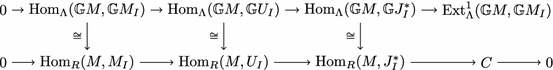
  Hence C is a submodule of $\mathrm{Ext}^1_\Lambda (\mathbb {G}M,\mathbb {G}M_I)$. But since (A.E) is exact, it follows that $e_IC=0$ and so C is a finitely generated $\Lambda _I$-module. Since $\Lambda _I$ has finite length, so too does C. But $\mathrm{depth}_R\mathrm{Ext}^1_\Lambda (\mathbb {G}M,\mathbb {G}M_I)>0$ since $\mathrm{Hom}_\Lambda (\mathbb {G}M,\mathbb {G}M_I)\cong \mathrm{Hom}_R(M,M_I)\in \mathrm{CM}\,R$, hence $C=0$.

• (2) If $\upnu _{I}M\cong M$, then $J_I^*\cong M_I$. Consequently, viewing the exact sequence in (1) as $\mathrm{End}_R(M)$-modules, the last term is projective and so the sequence splits. By reflexive equivalence this would imply that $M_I$ is a summand of $U_I\in \mathrm{add}\,M_{I^c}$, which is a contradiction.

• (3) Since the last map in (A.M) is a minimal right $\mathrm{add}\,M_{I^c}$-approximation, applying $\mathrm{Hom}_R(M,-)$ to (A.M) gives an exact sequence

  $$\begin{aligned} 0\rightarrow \mathrm{Hom}_R(M,J_I^*)\rightarrow \mathrm{Hom}_R(M,V_I)\rightarrow \mathrm{Hom}_R(M,M_I)\rightarrow \Lambda _{\mathrm {con}}^I\rightarrow 0. \end{aligned}$$

  Splicing this with the exact sequence in (1) gives the result.

• (4) If $d>3$, applying the depth lemma to the projective resolution in (3) gives a contradiction. $\square$

The above results give the following, stated in Sect. 2.3.

Corollary A.8

Suppose that $d\ge 3$, $\upnu _I \upnu _IM\cong M$ and $\dim _{\mathbb {C}}\Lambda _I<\infty$. As above, set $\Gamma :=\mathrm{End}_\Lambda (T_I)\cong \mathrm{End}_R(\upnu _IM)$. Then

• (1) $T_I\cong \mathrm{Hom}_R(M,\upnu _IM)$.

• (2) $\Omega _\Lambda ^2\Lambda _I=T_I$, thus $\mathrm {pd}_\Lambda \Lambda _I=3$ and $\mathrm{Ext}^1_\Lambda (T_I,-)\cong \mathrm{Ext}^3_\Lambda (\Lambda _I,-)$.

Proof

• (1) This follows from the definition of $T_I$, together with A.7(1).

• (2) This is now immediate from (1), A.7(1) and A.7(3).

$\square$

Appendix B: Conjectures

This appendix outlines conjectures and further directions. First and foremost, we are hampered by the fact that the Bridgeland–Chen flop functor is only known to be an equivalence in the setting of Gorenstein terminal singularities. This paper began by trying to lift the reconstruction algebra of [52] to 3-folds, and through the analysis of many non-Gorenstein examples. There is evidence to suggest the following.

Conjecture B.1

Suppose that $X\rightarrow X_{\mathrm {con}}$ is a flopping contraction of 3-folds, where X has at worst CM rational singularities. Then the flop functor is an equivalence if and only if the universal sheaf of the noncommutative deformation functor associated to the curves is a perfect complex (equivalently, $\mathrm {pd}_\Lambda \Lambda _{\mathrm {con}}<\infty$).

This would recover Bridgeland [5] and Chen [10], since when X has only Gorenstein terminal singularities, the universal sheaf is guaranteed to be perfect [15, 7.1].

Whilst mutation needs R to be Gorenstein to ensure that it gives a derived equivalence, it can sometimes be an equivalence when R is not Gorenstein. The relationship between flops and mutation seems to be tight.

Conjecture B.2

When $C_i$ is a crepant curve whose universal sheaf is perfect, and X has at worst CM rational singularities, then Theorem 1.2 remains true.

Conjecture B.3

The Homological MMP in Fig. 2 can be used to flop curves and jump between minimal models of non–Gorenstein singularities, again in the CM rational singularities setting, provided that we account for $\mathrm {pd}_\Lambda \Lambda _{\mathrm {con}}<\infty$.

Even although $\mathrm {pd}_\Lambda \Lambda _{\mathrm {con}}<\infty$ seems necessary to relate mutation to flops, it does not seem so relevant for moduli tracking purposes. The following is at least true in many examples, and may be true more generally.

Conjecture B.4

The moduli tracking theorem 5.12 is true under the simplifying assumption $\upnu _I\upnu _IM\cong M$.

Tracking moduli in the non-Gorenstein setting is substantially harder, since even reasonable algebras like NCCRs need not be closed under derived equivalence.

In an algebraic direction, 4.10 should extend to the situation when R is not Gorenstein. There is a version of the Auslander–McKay Correspondence in dimension two when R is not Gorenstein [52, 53], obtained by replacing CM modules by Wunram’s notion of a special CM module [53]. There should be a three dimensional analogue of this.

Conjecture B.5

There is a notion of ‘special MM generator’ such that the Auslander–McKay Correspondence 4.10 holds for non–Gorenstein rational 3-fold singularities whose minimal models have fibres that are at most one-dimensional.

Of course, the above conjecture must also account for $\mathrm {pd}_\Lambda \Lambda _{\mathrm {con}}<\infty$, but again this is guaranteed if we restrict to those $\mathrm{Spec}\,R$ admitting minimal models with only Gorenstein terminal singularities.

Since the noncommutative deformations in Sect. 3 detect contractions for both flips and flops, and has no restriction on singularities, it is reasonable to speculate about modifying the Homological MMP to cover flips. Indeed, philosophically there we should not be changing the GIT stability, since there is no derived equivalence so we do not expect to be able to track the moduli back. Instead, we change the algebra, keeping the GIT fixed.

Conjecture B.6

In the setting of CM rational singularities, given $N=H^0(\mathcal {V}_X)$, there is some homological modification of mutation that produces $H^0(\mathcal {V}_{X'})$ where $X'$ is the flip. Consequently, the Homological MMP in Fig. 2 can be extended to cover both flips and flops.

References

Auslander, M.: Rational singularities and almost split sequences. Trans. Am. Math. Soc. 293(2), 511–531 (1986)
Bergh, P.A.: On the existence of cluster tilting objects in triangulated categories. J. Algebra 417, 1–14 (2014)
Bocklandt, R., Schedler, T., Wemyss, M.: Superpotentials and Higher Order Derivations. J. Pure Appl. Algebra 214(9), 1501–152 (2010)
Brenner, S., Butler, M.C.R.: A spectral sequence analysis of classical tilting functors. Handbook of Tilting Theory, London Math. Soc. Lecture Note Ser., vol. 332. Cambridge University Press, Cambridge, pp. 31–48 (2007)
Bridgeland, T.: Flops and derived categories. Invent. Math. 147(3), 613–632 (2002)
Bridgeland, T., Stern, D.: Helices on del Pezzo surfaces and tilting Calabi-Yau algebras. Adv. Math. 224(4), 1672–1716 (2010)
Burban, I., Iyama, O., Keller, B., Reiten, I.: Cluster tilting for one-dimensional hypersurface singularities. Adv. Math. 217(6), 2443–2484 (2008)
Cartan, H., Eilenberg, S.: Homological Algebra. Princeton Landmarks in Mathematics. Princeton University Press, Princeton (1999)
Cassens, H., Slodowy, P.: On Kleinian singularities and quivers. Singularities (Oberwolfach, 1996), pp. 263–288, Progr. Math., vol. 162. Birkhuser, Basel (1998)
Chen, J.-C.: Flops and equivalences of derived categories for threefolds with only terminal Gorenstein singularities. J. Differ. Geom. 61(2), 227–261 (2002)
Clemens, H., Kollár, J., Mori, S.: Higher Dimensional Complex Geometry, Astérisque, vol. 166. Société Mathématique de France, Paris (1988)
Craw, A.: The McKay Correspondence and Representations of the McKay Quiver. University of Warwick Ph.D. thesis, xviii + 134 pp (June 2001)
Craw, A., Ishii, A.: Flops of \(G\)-Hilb and equivalences of derived categories by variation of GIT quotient. Duke Math. J. 124(2), 259–307 (2004)
Dao, H., Huneke, C.: Vanishing of Ext, cluster tilting and finite global dimension of endomorphism rings. Am. J. Math. 135(2), 561–578 (2013)
Donovan, W., Wemyss, M.: Noncommutative deformations and flops. Duke Math. J. 165(8), 1397–1474 (2016)
Donovan, W., Wemyss, M.: Contractions and deformations, arXiv:1511.00406
Donovan, W., Wemyss, M.: Twists and braids for 3-fold flops. JEMS (accepted, 2016). arXiv:1504.05320
Donovan, W., Wemyss, M.: Noncommutative enhancements of contractions, arXiv:1612.01687
Gulliksen, T.H.: On the deviations of a local ring. Math. Scand. 47(1), 5–20 (1980)
Hirano, Y., Wemyss, M.: Faithful actions from hyperplane arrangements, arXiv:1612.02582
Iyama, O., Reiten, I.: Fomin-Zelevinsky mutation and tilting modules over Calabi-Yau algebras. Am. J. Math. 130(4), 1087–1149 (2008)
Iyama, O., Wemyss, M.: The classification of special Cohen Macaulay modules. Math. Z. 265(1), 41–83 (2010)
Iyama, O., Wemyss, M.: Maximal modifications and Auslander–Reiten duality for non-isolated singularities. Invent. Math. 197(3), 521–586 (2014)
Iyama, O., Wemyss, M.: Singular derived categories of \(\mathbb{Q}\)-factorial terminalizations and maximal modification algebras. Adv. Math. 261, 85–121 (2014)
Iyama, O., Wemyss, M.: Reduction of triangulated categories and Maximal Modification Algebras for \(cA_n\) singularities. Crelle (2015). https://doi.org/10.1515/crelle-2015-0031
Kalck, M., Iyama, O., Wemyss, M., Yang, D.: Frobenius categories, Gorenstein algebras and rational surface singularities. Compos. Math. 151(3), 502–534 (2015)
Karmazyn, J.: Quiver GIT for varieties with tilting bundles. Manuscr. Math. 154(1–2), 91–128 (2017)
Katz, S.: Small resolutions of Gorenstein threefold singularities. Algebraic geometry: Sundance 1988, pp. 61–70, Contemp. Math., vol. 116, Am. Math. Soc., Providence, RI (1991)
Kawamata, Y., Matsuda, K., Matsuki, K.: Introduction to the minimal model problem. Algebraic geometry, Sendai, 1985, pp. 283–360, Adv. Stud. Pure Math., vol. 10, North-Holland, Amsterdam (1987)
Kawamata, Y., Matsuki, K.: The number of the minimal models for a 3-fold of general type is finite. Math. Ann. 276(4), 595–598 (1987)
Keller, B.: Derived categories and tilting. Handbook of tilting theory, pp. 49–104, London Math. Soc. Lecture Note Ser., vol. 332. Cambridge University Press, Cambridge (2007)
King, A.D.: Moduli of representations of finite-dimensional algebras. Quart. J. Math. Oxf. Ser. (2) 45(180), 515–530 (1994)
Kollár, J.: Flops. Nagoya Math. J. 113, 15–36 (1989)
Kollár, J.: Flips, flops, minimal models etc. Surveys in differential geometry (Cambridge, MA, 1990), pp. 113–199. Lehigh Univ, Bethlehem, PA (1991)
Kollár, J., Mori, S.: Classification of three-dimensional flips. J. Am. Math. Soc. 5(3), 533–703 (1992)
Kronheimer, P.B.: The construction of ALE spaces as hyper-Kähler quotients. J. Differ. Geom. 29(3), 665–683 (1989)
Laudal, O.A.: Noncommutative deformations of modules. The Roos Festschrift volume, 2. Homology Homotopy Applications, vol. 4(2), part 2, pp. 357–396 (2002)
Muto, T., Tani, T.: Stability of quiver representations and topology change. J. High Energy Phys. 2001(9), 8 (2001)
Nolla de Celis, A., Sekiya, Y.: Flops and mutations for crepant resolutions of polyhedral singularities. Asian J. Math. 21(1), 1–46 (2017)
Orlov, D.: Formal completions and idempotent completions of triangulated categories of singularities. Adv. Math. 226(1), 206–217 (2011)
Pinkham, H.: Factorization of birational maps in dimension 3. Singularities (P. Orlik, ed.), Proc. Symp. Pure Math., vol. 40, Part 2, pp. 343–371. American Mathematical Society, Providence (1983)
Ramras, M.: Maximal orders over regular local rings of dimension two. Trans. Am. Math. Soc. 142, 457–479 (1969)
Reid, M.: Minimal models of canonical 3-folds. Algebraic varieties and analytic varieties (Tokyo, 1981), pp. 131–180. Adv. Stud. Pure Math., 1, North-Holland, Amsterdam (1983)
Schröer, S.: A characterization of semiampleness and contractions of relative curves. Kodai Math. J. 24(2), 207–213 (2001)
Sekiya, Y., Yamaura, K.: Tilting theoretical approach to moduli spaces over preprojective algebras. Algebr. Represent. Theory 16(6), 1733–1786 (2013)
Toda, Y.: Stability conditions and crepant small resolutions. Trans. Am. Math. Soc. 360(11), 6149–6178 (2008)
Toda, Y.: On a certain generalization of spherical twists. Bull. Soc. Math. France 135(fascicule 1), 119–134 (2007)
Toda, Y.: Noncommutative width and Gopakumar-Vafa invariants. Manuscr. Math. 148(3–4), 521–533 (2015)
Van den Bergh, M.: Three-dimensional flops and noncommutative rings. Duke Math. J. 122(3), 423–455 (2004)
Van den Bergh, M.: Non-commutative crepant resolutions. The legacy of Niels Henrik Abel, pp. 749–770. Springer, Berlin (2004)
Weibel, C.A.: An introduction to homological algebra. Cambridge Studies in Advanced Mathematics, vol. 38. Cambridge University Press, Cambridge (1994). xiv+450 pp
Wemyss, M.: The GL(2,\(\mathbb{C} \)) McKay correspondence. Math. Ann. 350(3), 631–659 (2011)
Wunram, J.: Reflexive modules on quotient surface singularities. Math. Ann. 279(4), 583–598 (1988)
Acknowledgements
It is a pleasure to thank Alastair Craw and Alastair King for many discussions and comments over the eight years since this work began, and to thank Will Donovan and Osamu Iyama for many discussions and ideas, some of which are included here, and for collaborating on the foundational aspects [15,16,17, 23,24,25]. It is also a pleasure to thank the referee for many helpful comments and suggestions. Thanks are also due to Gavin Brown, Alvaro Nolla de Celis, Hailong Dao, Eleonore Faber, Martin Kalck, Joe Karmazyn, Miles Reid and Yuhi Sekiya.
Author information
Authors and Affiliations
Corresponding author
Additional information
The author was supported by EPSRC Grant EP/K021400/1.