Model Checking MANETs with Arbitrary Mobility

Abstract.

Modeling arbitrary connectivity changes of mobile ad hoc networks (MANETs) makes application of automated formal verification challenging. We introduced constrained labeled transition systems (CLTSs) as a semantic model to represent mobility. To model check MANET protocol with respect to the underlying topology and connectivity changes, we here introduce a branching-time temporal logic interpreted over CLTSs. The temporal operators, from Action Computation Tree Logic with an unless operator, are parameterized by multi-hop constraints over topologies, to express conditions on successful scenarios of a MANET protocol. We moreover provide a bisimilarity relation with the same distinguishing power for CLTSs as our logical framework.

These keywords were added by machine and not by the authors. This process is experimental and the keywords may be updated as the learning algorithm improves.

1 Introduction

In mobile ad hoc networks (MANETs), nodes communicate along multi-hop paths using wireless transceivers. Wireless communication is restricted; only nodes located in the range of a transmitter receive data. Due to e.g. noise in the environment, interferences, and temporary communication link errors, wireless communication is unreliable, which together with mobility of nodes complicates the design of MANET protocols. Formal methods provide valuable tools to design, evaluate and verify such protocols.

We introduced Restricted Broadcast Process Theory (RBPT) [9] to specify and verify MANETs, taking into account mobility. RBPT specifies a MANET by composing nodes using a restricted local broadcast operator. A strong point of RBPT is that the underlying topology is not specified in the syntax, which would make it hard to set up the initial topology for each scenario in a verification. In similar approaches, the mobility is modeled as arbitrary manipulation of the underlying topology (given as part of the semantic state), which may make the model infinite and insusceptible to automated verification techniques. Instead in the semantic model of RBPT, a constraint labeled transition system (CLTS) [10], transitions are enriched with so-called network constraints, to restrict the possible topologies. This symbolic representation of network topologies in the semantics is more compact and allows automated verification techniques to investigate families of properties on a unified model.

Properties in MANETs tend to be weaker than in wired networks, due to the topology-dependent behavior of communication, and consequently the need for multi-hop communication between nodes. For instance, an important property in routing or information dissemination protocols is packet delivery: If there exists an end-to-end route between two nodes $A$ and $B$ for a long enough period of time, then packets sent by $A$ will be received by $B$ [7]. To reason about properties that require such topology conditions, we introduce a temporal logic CACTL based on ACTLW [16], which consists of Action CTL [3] with an until operator. Our approach supports flexibility in verifying topology-dependent behavior (without changing the model), and restricting the generality of mobility as opposed to existing approaches. CACTL is interpreted over CLTSs. Path operators are parameterized with multi-hop constraints over the underlying topologies. We present a model checking algorithm for CACTL; a model checker for CACTL is being implemented, using the rewrite logic Maude. This provides a framework, supporting both equational reasoning [9] and model checking of MANET protocols, to verify topology-dependent properties like “existence of a route”.

We moreover introduce a novel notion of branching network bisimilarity, based on branching bisimilarity [24], that induces the same identification of CLTSs as CACTL. This relation is finer than the one introduced in [10], due to reliability of communication: A receiving node is not equivalent to a deadlocked node anymore, since in parallel with a sending node, an unsuccessful communication cannot be matched to a communication with no enabled receiver (which is the case in the lossy framework).

2 Related Work

MANET protocols have been studied either using existing formalisms such as SPIN [1, 5, 26] and UPPAAL [8, 15, 26, 27], or introducing specific frameworks mainly with an algebraic approach [7, 13, 14, 17, 18, 20, 21, 23]. Important modeling challenges in MANETs are local broadcast, underlying topology and mobility. The modeling approach using existing formalisms can be summarized as follows: The underlying topology is modeled by a two-dimensional array of Booleans, mobility by explicit manipulation of this matrix, and local broadcast by unicasting to all nodes with whom the sending node is presently connected, using the connectivity matrix. The verification approach tends to be based on model checking techniques restricted to a pre-specified mobility scenario. Lack of support for compositional modeling and arbitrary topology changes has motivated new approaches with a primitive for local broadcast and support of arbitrary mobility. These approaches are CBS#, bKlaim, CWS, CMAN, CMN, $\omega$-calculus, RBPT, CSDT, and AWN [7, 9, 13, 14, 17, 18, 20, 21, 23]. The common point among them (except RBPT) is implicit manipulation of the underlying topology in the semantics to model arbitrary connectivity changes and mobility. The analysis techniques supported by these frameworks, except bKlaim and AWN, are based on a behavioral congruence relation. In [10] we provided an axiomatization to derive that a specification of a MANET protocol is observably equal to a specification of its desired external behavior. Equational reasoning (applied at the syntactic or the semantic level) requires either abstraction from the actual specification of the MANET protocol, or knowledge about the overall behavior of the MANET beforehand. The model checking approach is useful to investigate specific properties of MANET protocols with less effort and knowledge. The mix of broadcast behavior and mobility leads to state-space explosion, hampering the application of automated verification techniques like model checking. In bKlaim [21], the semantic model is abstracted to a finite labeled transition system such that the mobility information is preserved; a variant of ACTL is introduced to determine which properties hold if movement of nodes is restricted. To this aim, ACTL operators are parameterized by a set of possible network configurations (topology). However, topology-dependent behavior cannot be checked. AWN [7] verifies topology-dependent behavior properties using CTL [2], by treating a transition label carrying (dis)connectivity information as a predicate of its succeeding state [7] and defining predicates over the topology as part of the syntax. This approach can be extended to algebras, e.g. CMAN and $\omega$-calculus, with (dis)connectivity information on transition labels. However, this approach needs auxiliary strategies to extract predicates from the states and transitions, to restrict connectivity changes during model checking and thus limit the state space. These challenges are tackled with the help of the model checker UPPAAL, by transforming AWN specifications to automata and exploiting an auxiliary automaton which statically restricts connectivity changes [8], similar to [15].

3 Background

Communication in wireless networks tends to be based on local broadcast: Only nodes that are located in the transmission area of a sender can receive. A node $B$ is directly connected to a node $A$, if $B$ is located within the transmission range of $A$. This asymmetric connectivity relation between nodes introduces a topology concept. A topology is a function $\gamma :{ Loc}\rightarrow {I\!\!P}({ Loc}$) where ${ Loc}$ denotes a finite set of (hardware) addresses $A,B,C$. We extend ${ Loc}$ with the unknown address $?$ to model open communications, which is helpful in giving semantics to MANETs in a compositional way.

Constrained labeled transition systems (CLTSs) [10] provide a semantic model for the operational behavior of MANETs. A transition label is a pair of an action and a network constraint, restricting the range of possible underlying topologies. A network constraint $\mathcal C$ is a set of connectivity pairs $\rightsquigarrow : { Loc}\times { Loc}$, where only the first address can be $?$. In this setting, non-existence of connectivity information between two addresses in a network constraint can imply three consequences; we do not have any information about the link (this is helpful when the link has no effect on the evolution of a network), the link was disconnected, or the link exists, but due to unreliable communication, the communication was unsuccessful. To distinguish these cases from each other, we extend the network constraints of CLTSs with a set of disconnectivity pairs $\mathrel {\not \rightsquigarrow }: { Loc}\times { Loc}$; while $B\rightsquigarrow A$ denotes that $A$ is connected to $B$ directly and consequently $A$ can receive data sent by $B$, $B\mathrel {\not \rightsquigarrow }A$ denotes that $A$ is not connected to $B$ directly and consequently cannot receive any message from $B$. In this setting, non-existence of connectivity information between two addresses in a network constraint means a lack of information. We write $\{B\rightsquigarrow A,C~-~B\mathrel {\not \rightsquigarrow }D,E\}$ instead of $\{B\rightsquigarrow A,B\rightsquigarrow C,B\mathrel {\not \rightsquigarrow }D, B\mathrel {\not \rightsquigarrow }E\}$.

A network constraint $\mathcal C$ is said to be well-formed if $\forall \ell \rightsquigarrow \ell '\in \mathcal C \,(\ell '\ne ?\wedge \ell \mathrel {\not \rightsquigarrow }\ell '\mathrel {\not \in }\mathcal C )$ and $\forall \ell \mathrel {\not \rightsquigarrow }\ell '\in \mathcal C \,(\ell '\ne ?\wedge \ell \rightsquigarrow \ell '\mathrel {\not \in }\mathcal C )$. Let $\mathbb C$ denote the set of well-formed network constraints that can be defined over network addresses in ${ Loc}$. Each network constraint $\mathcal C$ represents the set of network topologies that satisfy the (dis)connectivity pairs in $\mathcal C$, i.e., $\{ \gamma \mid \mathcal C \subseteq \mathcal C _{\Gamma }(\gamma ) \}$, where $\mathcal C _{\Gamma }(\gamma )$ extracts all one-hop (dis)connectivity information from $\gamma$. So the empty network constraint $\{\}$ denotes all possible topologies over ${ Loc}$. Let ${ Act}_\tau$ be the set of actions (including the silent action $\tau$), ranged over by $\eta$.

A CLTS is of the form by $\langle S,\Lambda ,\rightarrow ,s_0\rangle$, with $S$ a set of states, $\Lambda \subseteq \mathbb C \times { Act}_\tau$, $\rightarrow \,\subseteq S\times \Lambda \times S$ a transition relation, and $s_0\in S$ the initial state. A transition $(s,(\mathcal C ,\eta ),s')\in \,\rightarrow$, denoted by , expresses that a MANET protocol in state $s$ with an underlying topology $\gamma \in \mathcal C$ can perform action $\eta$ to evolve to state $s'$. Extending network constraints with disconnectivity pairs enables us to define different behaviors for the communication primitive (see Fig. 1). Furthermore, it allows us to reason about existence of a communication path between nodes, as will be explained in Section 4.1.

Fig. 1

Modeling different communication behaviors: $s_0$ represents a state in which $A$ broadcasts its data, while $s_1$ represents a state in which data has been transferred from $A$ to $B$

4 Constrained Action Computation Tree Logic

Properties of MANETs tend to be weaker than of wired networks, due to topology-dependent behavior of communication, and consequently the requirement of existence of a multi-hop communication path between nodes. CLTSs provide a suitable platform to verify topology-dependent properties, using the (dis)connectivity information encoded into the transition labels: While transitions are traversed to investigate a behavioral property, (dis)connectivity information is collected to verify the topology conditions on which the behavior depends. To this aim, we introduce a temporal logic based on Action CTL (ACTL) [3] which includes the until and next operators from CTL [2], parameterized with a set of actions. Recently a more expressive variant of ACTL called ACTLW [16] was introduced, in which the next is replaced by an unless operator.

4.1 Concepts

Since the behavior of MANET protocols depends on the underlying topology of the network, many properties depend on constraints on this topology. For example, to examine whether a routing protocol can find a route from node $A$ to node $B$, the existence of a multi-hop path from $A$ to $B$ is a pre-condition. Viewing a network topology as a directed graph, the simplest form of constraint consists of the (non-)existence of multi-hop relations between nodes.

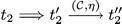
As explained in Section 3, states in a CLTS do not hold information about the underlying topology. E.g., from the transition sequence we can infer that at the moment we reach $t_1$, $B$ was connected to $A$, and at the moment we reach $t_2$, $C$ was connected to $B$. So we can conclude that to reach $t_2$ via this path, two links must exist (not essentially at the same time). That is, a multi-hop communication link from $A$ to $C$, denoted by $A\dashrightarrow C$, must exist to reach $t_2$. In general, to examine a property pre-conditioned by a multi-hop constraint over the topology, we look for a path in the CLTS along which the multi-hop relations are inferred.

Let $T=\langle S,\Lambda ,\rightarrow ,s_0\rangle$ be a CLTS. A path $\sigma$ of $T$ is a sequence of transitions $t_0 (\mathcal C _0,\eta _0) t_1 (\mathcal C _1,\eta _1) t_2 \ldots$ where $\forall i\ge 0\,((t_{i-1} (\mathcal C _{i},\eta _i) t_i)\in \,\rightarrow )$. A path is said to be maximal if it either is infinite or ends in a deadlock state.

When a multi-hop relation is the pre-condition of a property, we are stating a set of single-hop links (leading to a multi-hop connection) required for a set of communications. Inversely, we can infer from the network constraints of such communications over a path that the multi-hop connection exists. To this aim, we determine multi-hop connections by collecting single-hop constraints along a path in a forward fashion using a set of computations over network constraints. The operator $\oplus :\mathbb C \times \mathbb C \rightarrow \mathbb C$ allows to gather information along a path in a CLTS. It merges connectivity information, where the second argument overwrites conflicting information of the first argument:

$$\begin{aligned} \mathcal C _1\oplus \mathcal C _2 = \mathcal C _2 \cup \{ p \mid \lnot p \mathrel {\not \in }\mathcal C _2\wedge p\in \mathcal C _1\} \end{aligned}$$

where $\lnot (\ell \rightsquigarrow \ell ')=\ell \mathrel {\not \rightsquigarrow }\ell '$ and $\lnot (\ell \mathrel {\not \rightsquigarrow }\ell ')=\ell \rightsquigarrow \ell '$. This operator is left-associative and non-commutative; $\{\}$ is its identity element. Let $\oplus _{k=i}^j\mathcal C _k$ denote $(\ldots ((\mathcal C _{k=i}\oplus \mathcal C _{k=i+1})\oplus \mathcal C _{k=i+2})\ldots \oplus \mathcal C _{k=j})$. We say $\xi \in \mathbb C$ conforms to $\mathcal C$ if $\xi$ does not include (dis)connectivity information that contradicts $\mathcal C$, which can be formally tested by $\mathcal C \subseteq \mathcal C \oplus \xi$. Extending CLTSs with disconnectivity pairs allows to correctly update topology information gathered along a path when the communication behavior distinguishes lossy from disconnectivity by providing precise information in the labels (see Fig. 1(b) and 1(c)) in the case of unsuccessful communication. For instance, updating the connectivity information $\{A\rightsquigarrow B,C~-~B\rightsquigarrow C\}$ with $A\mathrel {\not \rightsquigarrow }B$ results in $\{A\rightsquigarrow C,B\rightsquigarrow C,A\mathrel {\not \rightsquigarrow }B\}$.

A path $t_0 (\mathcal C _0,\eta _0) t_1 (\mathcal C _1,\eta _1) t_2 \ldots$ is called $\mathcal C$-path if $\mathcal C _{i}$ conforms to $\mathcal C$ for all $i\ge 0$.

4.2 CACTL Syntax

To provide a logic to verify topology-dependent properties of MANET protocols, our modal path operator is parameterized with multi-hop constraints over the topology. This parameter specifies the pre-condition required for inspecting the property; if the pre-condition never holds, the property does not need to hold. Moreover, to verify properties of MANETs with regard to different mobility scenarios, the satisfaction relation is parameterized with single-hop constraints. This parameter expresses the (non-)existence of communication links and also restricts node mobility; nodes can only move in such a way that the specified links do not change. This is achieved by only traversing transitions that conform to the specified links. For instance, consider the CLTS in Fig. 2(a). We examine properties under the network constraint $\{B \mathrel {\not \rightsquigarrow }C\}$, meaning that $C$ is never in the transmission range of $B$. To this aim we should traverse transitions with network constraints $\mathcal C$ such that $\{B \mathrel {\not \rightsquigarrow }C\}\subseteq \{B \mathrel {\not \rightsquigarrow }C\}\oplus \mathcal C$ (like $s_0\rightarrow s_1\rightarrow s_3$ in the CLTS in Fig. 2(a)). This can be explained by partially unfolding the CLTS, as depicted in Fig. 2(b), with an initial topology $\gamma _0$ where $B\in \gamma _0(A)$, $D\in \gamma _0(B)$ and $C\mathrel {\not \in }\gamma _0(B)$. Three possible mobility scenarios of state $\langle s_1,\gamma _0\rangle$ are shown: One moves $C$ in the transmission range of $B$, while another moves $D$ out and $C$ in the transmission range of $B$. According to the mobility restriction, the resulting topologies $\gamma _1$ and $\gamma _2$ do not satisfy $\{B \rightsquigarrow C\}$. Therefore only the middle scenario to $\langle s_3,\gamma _0\rangle$ is possible.

Fig. 2

Restricted mobility, achieved through restricted transition traversal

Our logic borrows its temporal operators from ACTLW: $\mathbf {AU}$, $\mathbf {EU}$, $\mathbf {AW}$, and $\mathbf {EW}$. Let $\eta \in { Act}_\tau$, $\ell ,\ell '\in { Loc}$, $\mathcal C \in \mathbb C$. Action formula $\chi$, topology formula $\mu$, state formula $\phi$ (also called CACTL formula), and path formula $\psi$ are defined by the grammars:

While action and state formulae are the same as in ACTLW, path formulae carry a condition over topologies. Intuitively, a path formula $\phi {~}_{\{\chi \}}\mathbf U {~}^{\mu } {\!}_{\{\chi '\}}\phi '$ specifies a path along which states satisfying property $\phi$ perform actions from $\chi$, until the accumulated (dis)connectivity information along this path satisfies the topology formula $\mu$, and a state satisfying property $\phi '$ is reached after an action from $\chi '$. An infinite path that never stabilizes to a situation where $\mu$ is always satisfied, still satisfies this path formula if all its states satisfy $\phi$ and all its transitions are from $\chi$. But if a path does stabilize to such a situation, then eventually a transition from $\chi '$ must lead to a state where $\phi '$ holds. Typically, $\mu$ could define that there is a path from node $A$ to node $B$, and $\phi '$ could define that some information broadcast by $A$ reaches $B$.

The path formula based on the unless (weak until) operator $\phi {~}_{\{\chi \}}\mathbf W {~}^{\mu } {\!}_{\{\chi '\}}\phi '$ specifies a path along which states satisfying property $\phi$ perform actions from $\chi$ at least as long as either $\mu$ is never satisfied or no state satisfying $\phi '$ is visited by an actions from $\chi '$. We note that $\mathbf {EW}$ cannot readily be defined in terms of $\mathbf {AU}$ as opposed to CTL, due to actions of $\chi$ and $\chi '$ that should be visited to reach states satisfying $\phi$ and $\phi '$.

4.3 CACTL Semantics

Let $\eta '\in { Act}_\tau$, $\zeta \in \mathbb C$, and $\langle S,\Lambda ,\rightarrow ,s_0\rangle$ a CLTS. Satisfaction under network constraint $\zeta$ of action formula $\chi$ by $\eta \in { Act}_\tau$ (written $\eta \models _{\zeta } \chi$), topology formula $\mu$ by network constraint $\mathcal C$ (written $\mathcal C \models _\zeta \mu$), state formula $\phi$ by state $t$ (written $t\models _\zeta \phi$), or path formula $\psi$ by maximal path $\sigma$ (written $\sigma \models _\zeta \psi$), is inductively defined below. Let $\sigma ^s_i$, $\sigma ^\mathcal{C }_i$ and $\sigma ^\eta _i$ denote the $i$-th state, network constraint and action on path $\sigma$. With $\oplus _{k=1}^{\infty }\sigma ^\mathcal C _k\nvDash _\zeta \mu$ we mean that $\oplus _{k=1}^{m}\sigma ^\mathcal C _k\models _\zeta \lnot \mu$ for infinitely many $m\ge 1$.

$$\begin{aligned} & \eta \models _{\zeta }{ true}&\text {always} \\ & \eta \models _{\zeta }&\eta^{\prime} \text { iff }\eta =\eta^{\prime}\\ &\eta \models _{\zeta }&\lnot \chi \text { iff }\eta \nvDash _{\zeta } \chi \\ & \eta \models _{\zeta }&\chi \wedge \chi^{\prime} \text { iff }\eta \models _\zeta \chi \wedge \eta \models _\zeta \chi^{\prime}\\ & \mathcal C \models _\zeta{ true} &\text { always}\\ & \mathcal C \models _\zeta \ell \dashrightarrow \ell^{\prime} &\text { iff there are } \ell _0,\ldots ,\ell _n\in { Loc}\text{ with } \ell _0=\ell ,\, \ell _n=\ell^{\prime},\text{ and}\\&&\ell _i\rightsquigarrow \ell _{i+1}\in \zeta \oplus \mathcal C \text{ for all } i=0,\ldots ,n-1\\ & \mathcal C \models _\zeta \lnot \mu &\text { iff } \mathcal C \nvDash _\zeta \mu \\& \mathcal C \models _\zeta \mu \wedge \mu ^{\prime} &\text { iff } \mathcal C \models _\zeta \mu \wedge \mathcal C \models _\zeta \mu^{\prime } \\ & t\models _{\zeta }{ true} &\text { always}\\ & t\models _{\zeta } \lnot \phi &\text { iff } t \nvDash _{\zeta }\phi \\& t\models _{\zeta }\phi \wedge \phi^{\prime} &\text { iff } t\models _{\zeta }\phi \wedge t\models _{\zeta }\phi^ {\prime} \\& t\models _{\zeta } \mathbf E \psi &\text { iff there exists a maximal } \zeta -\text{path } \sigma \text{ such that } t=\sigma ^s_0\wedge \sigma \models _{\zeta }\psi \\& t\models _{\zeta } \mathbf A \psi &\text { iff for all maximal } \zeta -\text{paths } \sigma , \, t=\sigma ^s_0\Rightarrow \sigma \models _{\zeta }\psi \\& \sigma \models _{\zeta }\phi {~}_{\{\chi \}}\mathbf U {~}^{\mu } {\!}_{\{\chi^ \prime \}}\phi ^ \prime &\text { iff } \sigma ^s_0 \models _{\zeta } \phi , \text{ and either } \oplus _{k=1}^{\infty }\sigma ^\mathcal C _k\nvDash _\zeta \mu , \forall j\ge 1\,(\sigma ^s_j\models _\zeta \phi \,\wedge \\ & \qquad \qquad (\sigma ^\eta _j\models _\zeta \chi \wedge \zeta \subseteq \zeta \oplus \sigma ^\mathcal C _j )\vee (\sigma ^\eta _j=\tau \wedge \sigma ^\mathcal C _j=\{\}))) \text{ or there exists an } i\ge 1 \\ & \qquad \text { such that } \sigma ^s_i\models _{\zeta \oplus (\oplus _{k=1}^{i}\sigma ^\mathcal C _k)} \phi ^{\prime} , \sigma ^\eta _i\models _\zeta \chi \prime, \zeta \subseteq \zeta \oplus \sigma _i^\mathcal{C }, \oplus _{k=1}^{i}\sigma ^\mathcal C _k\models _\zeta \mu , \text{ and}\\ & \qquad \forall 1\le j<i\,( \sigma ^s_j\models _\zeta \phi \wedge ((\sigma ^\eta _j\models _\zeta \chi \wedge \zeta \subseteq \zeta \oplus \sigma ^\mathcal C _j )\vee (\sigma ^\eta _j=\tau \wedge \sigma ^\mathcal C _j=\{\}))) \\ &\sigma \models _{\zeta } \phi {~}_{\{\chi \}}\mathbf W {~}^{\mu } {\!}_{\{\chi ^{\prime} \}}\phi^{\prime} &\text { iff } \sigma \models _{\zeta }\phi {~}_{\{\chi \}}\mathbf U {~}^{\mu } {\!}_{\{\chi ^{\prime} \}}\phi^{\prime}, \text{ or } \sigma ^s_0 \models _{\zeta } \phi \text{ and }\forall j\ge 1\,( \sigma ^s_j\models _\zeta \phi \\ &\quad{ \wedge \,((\sigma ^\eta _j\models _\zeta \chi \wedge \zeta \subseteq \zeta \oplus \sigma ^\mathcal C _j)\vee (\sigma ^\eta _j=\tau \wedge \sigma ^\mathcal C _j=\{\})))}\end{aligned}$$

We use $\models$ to denote $\models _{\{\}}$ and ${~}_{\{\chi \}}\mathbf U {~}^{~} {\!}_{\{\chi '\}}$ to denote ${~}_{\{\chi \}}\mathbf U {~}^{ true} {\!}_{\{\chi '\}}$. We remark that the semantics of the until operator is somewhat different from CTL: $\mathbf E (\phi {}_{\{\chi \}} \mathbf U {}_{\{\chi '\}} \phi ')$ in ACTLW (similar to ACTL) requires to perform at least one action from $\{\chi '\}$ to reach a state satisfying $\phi '$, while $\mathbf E (\phi \mathbf U \phi ')$ in CTL is satisfied if the first state satisfies $\phi '$. Furthermore, our semantics explicitly distinguishes silent actions $\tau$ (over all possible topologies) and visible actions (similar to ACTL, in contrast to ACTLW).

For example, the state formula $\mathbf A ({ true}{~}_{\{\tau \vee { init}\}}\mathbf U {~}^{A\dashrightarrow B} {\!}_{\{{ get}\}}{ true})$ indicates that if there exists a path from $A$ to $B$, the action ${ init}$ is followed by action ${ get}$, after some communication (specified by $\tau$). E.g., the path

satisfies $({ true}{~}_{\{\tau \vee { init}\}}\mathbf U {~}^{A\dashrightarrow B} {\!}_{\{{ get}\}}{ true})$ with no restriction on mobility of nodes ($\zeta =\{\}$), since $get$ is observed after passing transitions with labels of ${ init}$ and $\tau$, and the accumulated network constraints over these transitions, $\{\}\oplus \{A\rightsquigarrow C~-~ A\mathrel {\not \rightsquigarrow }B,D\}\oplus C\rightsquigarrow D~-~C\mathrel {\not \rightsquigarrow }A,B\}\oplus \{D\rightsquigarrow B~-~D\mathrel {\not \rightsquigarrow }C\}\oplus \{\}$ induces that $A\dashrightarrow B$ via $C$ and $D$.

4.4 CACTL Model Checking

We adapt the CTL model checking algorithm (see [6]) to CACTL. Model checking a CACTL formula $\varphi$ under $\zeta \in \mathbb C$ starts with smallest sub-formulae and works outwards toward $\varphi$. The model checking will operate by adding to each state a set of labels of the form $\langle \phi ,\Omega ,O\rangle$, where $\phi$ is a subformula of $\varphi$, $\Omega$ a set of (dis)connectivity pairs, not necessarily well-formed, and $O$ a set of topology obligations. The set $\Omega$ maintains the history of links experienced during exploration of $\varphi$, and is helpful in the verification of state formulae based on (weak) until operators. A topology obligation is a pair of a topology formula $\mu$ and a network constraint $\mathcal C$. A topology obligation $\langle \mu ,\mathcal C \rangle$ is said to be satisfied when $\mathcal C \models _\zeta \mu$. Initially all states are labeled by $\langle { true},\emptyset ,\emptyset \rangle$. A state satisfies $\varphi$ iff at the end it includes a label $\langle \varphi ,\Omega ,O\rangle$ with the topology obligations in $O$ all satisfied. The pseudo code of the model checking algorithm’s backbone is given in Fig. 3.

Fig. 3

Model checking algorithm

We explain the idea of procedure CheckEU for the $\mathbf {EU}$ operator; other CACTL operators can be dealt with in a similar way. The pseudo code of this procedure is given in Appendix A. For simplicity we assume that CLTSs are deadlock-free. We extend the application of $\oplus$ to topology obligations: $\mathcal C \oplus O=\{\langle \mu , \mathcal C \oplus \mathcal C '\rangle \mid \langle \mu , \mathcal C '\rangle \in O\}$. Two possible cases should be examined. In the first case, state $s$ satisfies formula $\mathbf E (\phi {~}_{\{\chi \}}\mathbf U {~}^{\mu } {\!}_{\{\chi '\}}\phi ')$ if there exists a path from $s$ consisting of states satisfying property $\phi$ under $\zeta$ and actions from $\chi$, until a state satisfying $\phi '$ under $\zeta \oplus \xi$ is reached after an action from $\chi '$ and $\xi$ induces $\mu$, where $\xi$ is the accumulated (dis)connectivity information along this path. To check this case, we move backward starting from the states where $\phi '$ holds under $\zeta$, first over a transition with an action from $\chi '$, and then over transitions with an action from $\chi$, passing over states where $\phi$ holds under $\zeta$. We record the status of links encountered during backward exploration of executions (note that these links conform to $\zeta$). To ensure conformability of the links recorded for $\phi '$ to $\zeta \oplus \xi$, we incrementally check conformability of these links to the partial of $\xi$ being formed in the backward exploration. Since the yet unknown $\xi$ should induce $\mu$, we initially include topology obligation $\langle \mu ,\{\}\rangle$ in the state label; its network constraint is incrementally updated while moving backward. Furthermore, we record the topology obligation generated during exploration of $\phi$ and $\phi '$. To ensure $\phi '$ holds under $\zeta \oplus \xi$, we incrementally update its recorded topology obligation while moving backward.

Let $\Omega$ and $\Omega '$ contain the links that occurred over executions during exploration of $\phi$ and $\phi '$, and $O$ and $O'$ the topology obligations generated during exploration of $\phi$ and $\phi '$ (under $\zeta$), respectively. Since first $\phi$ and only after that $\phi '$ needs to hold, these sets can be kept separate. The sets $\Omega$ and $\Omega '$ may contain conflicting conditions, and even if $\Omega '$ conforms to the partial of $\xi$, $\Omega \cup \Omega '$ may not. To check conformability of $\Omega '$ to and update $O'$ with partial $\xi$, we postpone mixing these sets until the end, and exploit a senary labeling $\langle \mathbf E (\phi {~}_{\{\chi \}}\mathbf U {~}^{\mu } {\!}_{\{\chi '\}}\phi '),\Omega ,\Omega ',\mathcal C ,O,O'\rangle$. Let $\mathcal C$ be the accumulated value of network constraints over the traversed execution path. By moving backward over a $(\mathcal C ,\eta )$-transition (where $\mathcal C$ conforms to $\zeta$ and $\eta$ satisfies $\chi '$) from the state labeled with $\langle \phi ',\Omega ',O'\rangle$ to the state labeled with $\langle \phi ,\Omega ,O\rangle$, we add the label $\langle \mathbf E (\phi {~}_{\{\chi \}}\mathbf U {~}^{\mu } {\!}_{\{\chi '\}}\phi '),\Omega \cup \mathcal C ,\Omega ',\mathcal C ,O,\{\langle \mu ,\mathcal C \rangle \}\cup \mathcal C \oplus O'\rangle$ to states labeled with $\langle \phi ,\omega ,O\rangle$, if $\Omega '$ conforms to $\mathcal C$; it should be noted that $\mathcal C$ is added to $\Omega$ (and $\Omega$ conforms to $\zeta$), $O'$ is updated with $\mathcal C$, and the obligation $\{\langle \mu ,\mathcal C \rangle \}$ ($\mathcal C \oplus \{\langle \mu ,\{\}\rangle \}$) is generated during model checking of $\mathbf E (\phi {~}_{\{\chi \}}\mathbf U {~}^{\mu } {\!}_{\{\chi '\}}\phi ')$. At the end of model checking, the senary labels $\langle \mathbf E (\phi {~}_{\{\chi \}}\mathbf U {~}^{\mu } {\!}_{\{\chi '\}}\phi '),\Omega ,\Omega ',\mathcal C ,O,O'\rangle$ are replaced by $\langle \mathbf E (\phi {~}_{\{\chi \}}\mathbf U {~}^{\mu } {\!}_{\{\chi '\}}\phi '),\Omega \cup \Omega ',O\cup O'\rangle$.

Next we continue moving backward from the states with labels of the form $\langle \mathbf E (\phi \\ {~}_{\{\chi \}}\mathbf U {~}^{\mu } {\!}_{\{\chi '\}}\phi '),\Omega ,\Omega ',\mathcal C ',O,O'\rangle$ over $(\{\},\tau )$ or $(\mathcal C ,\eta )$-transitions of which their action satisfies $\chi$ and their network constraint conforms to $\zeta$, to reach states labeled by $\langle \phi ,\Omega '',O''\rangle$ for some $\Omega ''$ and $O''$. We add the label $\langle \mathbf E (\phi {~}_{\{\chi \}}\mathbf U {~}^{\mu } {\!}_{\{\chi '\}}\phi '),\Omega \cup \Omega ''\cup \mathcal C ,\Omega ',\mathcal C \oplus \mathcal C ',O\cup O'',\mathcal C \oplus O'\rangle$ to these states, if $\Omega '$ conforms to $\mathcal C \oplus \mathcal C '$. We continue moving backward until no new label is added to the states.

Fig. 4

The CLTS to be checked for $\mathbf E ({ true}{~}_{\{a\vee \tau \}}\mathbf U {~}^{A\dashrightarrow B} {\!}_{\{b\}}\mathbf E ({ true}{~}_{\{a\vee \tau \}}\mathbf U {~}^{A\dashrightarrow C} {\!}_{\{c\}}$ true))

Table 1 Labels of states in Fig. 4 while checking formula $\varphi _2\equiv \mathbf E (\phi {~}_{\{a\vee \tau \}}\mathbf U {~}^{A\dashrightarrow B} {\!}_{\{b\}}\varphi _1)$, where $\varphi _1\equiv \mathbf E (\phi {~}_{\{\chi \}}\mathbf U {~}^{A\dashrightarrow C} {\!}_{\{c\}}\phi )$ and $\phi \equiv { true}$

As an example, we verify $\mathbf E ({ true}{~}_{\{a\vee \tau \}}\mathbf U {~}^{A\dashrightarrow B} {\!}_{\{b\}}\mathbf E ({ true}{~}_{\{a\vee \tau \}}\mathbf U {~}^{A\dashrightarrow C} {\!}_{\{c\}}{ true}))$ under $\{\}$ over the CLTS given in Fig. 4. States are initially labeled by $\langle { true},\emptyset ,\emptyset \rangle$. Table 1 includes the labels given to the states in each step; first we label states $\mathcal M _7$ to $\mathcal M _4$ for the inner until operator, and then we label states $\mathcal M _4$ to $\mathcal M _0$ for the outer until operator. State $\mathcal M _{1_2}$ is only labeled by $\langle { true},\emptyset ,\emptyset \rangle$ and cannot be labeled further, because the set of links encountered during exploration of the inner until formula, i.e. $\{B\rightsquigarrow C,D\rightsquigarrow C\}$, does not conform to $\{D\rightsquigarrow B,D\mathrel {\not \rightsquigarrow }C\}$. State $\mathcal M _0$ includes the label $\langle \varphi _2,\{D\rightsquigarrow B,A\rightsquigarrow D,B\rightsquigarrow C,D\rightsquigarrow C\},\{\langle A\dashrightarrow C,\{D\rightsquigarrow B,A\rightsquigarrow D,B\rightsquigarrow C,D\rightsquigarrow C\} \rangle ,\langle A\dashrightarrow B, \{D\rightsquigarrow B,A\rightsquigarrow D\}\rangle \}\rangle$, so it satisfies $\varphi _2$ (under $\{\}$), since $\{D\rightsquigarrow B,A\rightsquigarrow D,B\rightsquigarrow C,D\rightsquigarrow C\}\models A\dashrightarrow C$ and $\{D\rightsquigarrow B,A\rightsquigarrow D\}\models A\dashrightarrow B$. The topology formula $A\dashrightarrow C$ in the inner until formula is satisfied after the network constraints $A\rightsquigarrow D$ and $D\rightsquigarrow B$ update their corresponding topology obligation while moving backward to model check the outer formula.

In the second case, $s$ satisfies $\mathbf E (\phi {~}_{\{\chi \}}\mathbf U {~}^{\mu } {\!}_{\{\chi '\}}\phi ')$ if there exists a path from $s$ along which the states satisfy $\phi$, the actions are from $\chi$, and the accumulated (dis)connectivity information never induces $\mu$ permanently (see Fig. 5 for two simple examples). To check the occurrence of this case, we decompose the CLTS into non-trivial strongly connected components (SCCs), meaning that they contain at least one edge.

We first restrict to states that include a label $\langle \phi ,\Omega ,O\rangle$ for some $\Omega$ and $O$, and to $(\{\},\tau )$ and $(\mathcal C ,\eta )$-transitions where $\eta$ satisfies $\chi$ and $\mathcal C$ conforms to $\zeta$. Next, we partition the new CLTS into SCCs using the algorithm explained in [2]. We initially move backward in an SCC over $(\mathcal C ,\eta )$-transitions, and for any $\langle \phi ,\Omega _1,O_1\rangle \in { label}(s)$ and $\langle \phi ,\Omega _2,O_2\rangle \in { label}(t)$, where $s$ and $t$ are origin and destination of transition, we add the label $\langle \mathbf E (\phi {~}_{\{\chi \}}\mathbf U {~}^{\mu } {\!}_{\{\chi '\}}\phi '),\Omega _1\cup \Omega _2\cup \mathcal C ,\emptyset ,\mathcal C ,O_1\cup O_2,\{\langle \lnot \mu ,\mathcal C \rangle \}\rangle$ to $s$. The obligation $\langle \lnot \mu ,\mathcal C \rangle$ indicates that the accumulated value of network constraints does not induce $\mu$. Then, similar to first case, we move backward out of the SCC until no new label is added to the states, and at the end we replace senary labels by triples.

Fig. 5

Two examples of infinite execution paths for which the accumulated network constraints never induce $A\dashrightarrow B$ permanently

5 Protocol Analysis with CACTL

To illustrate the expressiveness of CACTL in the analysis of MANETs, we specify properties for two important classes of protocols, namely routing and leader election.

The most fundamental error in routing protocol operations is failure to route correctly. The correct operation of MANET routing protocols is defined as follows [26]: If from some point in time on there exists a path between two nodes, then the protocol must be able to find some path between the nodes. Furthermore, when a path has been found, and for the time it stays valid, it must be possible to send packets along the path from the source node to the destination node. To verify the first part of property, let ${ init}({ src})$ and ${ found}({ src})$ indicate initialization and completion respectively of the route discovery protocol in a node with address $src$ for a specific address $dst$. The property “whenever there exists a path from $src$ to $dst$ and from $dst$ to $src$, each ${ init}({ src})$ is proceeded by its corresponding ${ found}({ src})$”, for ${ scr}\in \{A,C\}$ and ${ dst}=B$, is specified by the CACTL formula

$$\begin{aligned} \begin{array}{l} \mathbf A ({ true}{~}_{\{\tau \vee { init}(A)\vee { init}(C)\}}\mathbf U {~}^{A\dashrightarrow B\wedge B\dashrightarrow A} {\!}_{\{{ found(A)}\}}{ true}) ~\wedge \\ \mathbf A ({ true}{~}_{\{\tau \vee { init}(C)\vee { init}(C)\}}\mathbf U {~}^{C\dashrightarrow B\wedge B\dashrightarrow C} {\!}_{\{{ found(C)}\} }{ true}) \end{array} \end{aligned}$$

where $\tau$ abstracts away from communications between nodes. By model checking the CLTS model of a MANET in which the nodes deploy a routing protocol, we can verify this property with respect to arbitrary topology changes. This property was examined in [7] for the AODV protocol using CTL.

To verify the second part of the property, let ${ insert}({ src})$ and ${ delivery}({ src})$ indicate submission and arrival of a data over the route found beforehand at $src$ and $dst$ respectively. The property “whenever there exists paths from $src$ to $dst$ and from $dst$ to $src$, when a route is found from $src$ to $dst$; and while this path is valid each ${ insert}$ is followed by ${ deliver}$”, for ${ src}=C$ and ${ dst}=B$, is specified by the CACTL formula

$$\begin{aligned} \mathbf A ({ true}{~}_{\{{ init}(C)\vee { init}(A) \vee \tau \}}\mathbf U {~}^{C\dashrightarrow B\wedge B\dashrightarrow C} {\!}_{\{{ found}(C)\}}(\mathbf A ({ true}{~}_{\{{ insert}\vee \tau \}}\mathbf U {~}^{ true} {\!}_{\{{ deliver}\}}{ true}))) \end{aligned}$$

The outer until formula looks for all maximal paths in which $found$ is performed after $init$ while the accumulated network constraints $\xi$ induce $C\dashrightarrow B$ and $B\dashrightarrow C$ (or this topology formula is never induced), and by $found$ reach a state of which all maximal $\xi$-paths satisfy the inner until path formula. The network constraints over a $\xi$-path do not violate the single-hop (dis)connectivity pairs in $\xi$. It can be said that (dis)connectivity pairs are frozen, and consequently the route from $src$ to $dst$ is still valid.

Classical leader election algorithms aim at electing a unique leader from a fixed set of nodes. In the context of MANETs such protocols should consider arbitrary topology changes, and aim at finding a unique leader which is the most-valued node within a connected component [25]. Let ${ leader}({ id},{ lid})$ indicate that a node with address $id$ has found its leader with address ${ lid}$, and let node $A$ be the most-valued node. We can investigate correctness of such a leader election algorithm with the CACTL formula

$$\begin{aligned} \begin{array}{l} \mathbf A ({ true}{~}_{{ Act}_\Lambda }\mathbf U {~}^{\tiny \begin{array}{l}A\dashrightarrow B\wedge A\dashrightarrow C\wedge \\ B\dashrightarrow A\wedge B\dashrightarrow C\wedge \\ C \dashrightarrow A\wedge C\dashrightarrow B\end{array}} {\!}_{\{{ leader}(A,A),{ leader}(B,A),{ leader}(C,A)\}}{ true}) \end{array} \end{aligned}$$

It expresses that in any connected component containing nodes $A$, $B$ and $C$, eventually $A$ is chosen as the leader. Being in the same connected component is indicated by the existence of multi-hop paths among them. We can also investigate scenarios in which two disconnected components merge together with the help of a CACTL formula like

$$\begin{aligned} \begin{array}{l} \mathbf A ({ true}{~}_{{ Act}_\Lambda }\mathbf U {~}^{\tiny \begin{array}{l}A\dashrightarrow B\wedge B\dashrightarrow A\wedge \\ C\dashrightarrow D\wedge D\dashrightarrow C\wedge \\ \lnot A\dashrightarrow C\wedge \lnot A\dashrightarrow D\wedge \\ \lnot B\dashrightarrow C\wedge \lnot B\dashrightarrow D\end{array}} {\!}_{\{{ leader}(A,A),{ leader}(B,A),{ leader}(D,C)\}}(\\ \qquad \qquad\mathbf A ({ true}{~}_{{ Act}_\Lambda }\mathbf U {~}^{C\dashrightarrow B\wedge B\dashrightarrow C} {\!}_{\{{ leader}(A,A),{ leader}(B,A),{ leader}(D,A),{ leader}(C,A)\}}{ true})) \end{array} \end{aligned}$$

meaning that nodes $A,B$ and nodes $C,D$ belong to the same component with leader $A$ and $C$ respectively; if these two components get connected via $B$ and $C$, then they will eventually converge to the same leader, i.e. $A$.

6 Branching Network Bisimilarity

We define a novel notion of branching network bisimilarity that induces the same identification of CLTSs as our logical framework.

Definition 1.

Let $\langle S,\Lambda ,\rightarrow ,s_0\rangle$ be a CLTS. States $r,s\in S$ are logically equivalent, denoted by $r\sim _{L}s$, iff $\forall \zeta \in \mathbb C ~\forall \varphi \in { CACTL}~(r\models _\zeta \varphi \Leftrightarrow s\models _\zeta \varphi )$.

Intuitively, equivalent states in a CLTS exhibit the same behavior for any topology. This behavior includes communication and internal actions. Communication actions carry a message and the address of the sender, which can be abstracted into the unknown address $?$. Two equivalent states must match on every internal action, receive action, and send action with a known address. A send action with unknown address can be mimicked by a send action with either a known or unknown address. Let $\Longrightarrow$ denote the reflexive-transitive closure of $\tau$-transitions, over all possible topologies.

Definition 2.

A binary relation $\mathcal R$ on states in a CLTS is a branching network simulation if $t_1\mathcal R t_2$ and implies that:

• either $(\mathcal C ,\eta )$ is $(\{\},\tau )$, and $t_1'\mathcal R t_2$; or

• there are $t_2'$ and $t_2''$ such that , where $t_1\mathcal R t_2'$ and $t_1'\mathcal R t_2''$; or

• $\eta \equiv { nsnd}(\mathfrak m ,?)$, and there are $t_2'$, $t_2''$ and $\ell$ such that , where $t_1\mathcal R t_2'$ and $t_1'\mathcal R t_2''$.

$\mathcal R$ is a branching network bisimulation if $\mathcal R$ and $\mathcal{R }^{-1}$ are branching network simulations. Two terms $t_1$ and $t_2$ are branching network bisimilar, denoted by $t_1 \simeq _{b} t_2$, if $t_1\mathcal R t_2$ for some branching network bisimulation relation $\mathcal R$.

Theorem 1.

$\simeq _{b}$ is an equivalence relation.

This theorem can be proved in a similar fashion as for branching computed network bisimilarity in [9]. As said, branching network bisimilarity and the equivalence relation induced by CACTL coincide. This can be proved for CLTSs with so-called bounded-nondeterminism following the approach of [4]. The result can be lifted to general CLTSs in the same vein as [19], by resorting to infinitary logics (see [11] for the proof).

Theorem 2.

Let $\langle S,\Lambda ,\rightarrow ,s_0\rangle$ be a CLTS. For any $r,s\in S$, $r\simeq _{b}s$ iff $r\sim _L s$.

7 Conclusion and Future Work

We introduced the branching-time temporal logic CACTL, interpreted over CLTSs, to reason about topology-dependent behavior of MANET protocols. We can investigate scenarios like after a route found and after two disconnected components merged with the help of multi-hop constraints over topologies, which are specified as a part of path operators in our logic. Advantages of our approach are flexibility in verifying topology-dependent behavior (without changing the model), and restricting the generality of mobility. By nesting until operators, a specific path can be found with the help of topology constraints (without a need to specify how a topology constraint should be inferred), and then fixed for further exploration. The (dis)connectivity information in CLTS transitions makes it possible to restrict the generality of mobility as desired. By contrast, in approaches like [7], the inferences leading to the establishment of topology constraints should be embedded in the specification. Existing approaches to model mobility either are insusceptible to model checking [7, 13, 23], or require separate modeling of mobility [8]. The logic in [21] does not support verification of topology-dependent behavior.

A model checker for CACTL is being implemented, using the rewrite logic Maude. We also intend to verify real-world MANET protocols.

A   Pseudo Code of Procedure CheckEU

References

Bhargavan, K., Obradovid, D., Gunter, C.A.: Formal verification of standards for distance vector routing protocols. Journal of the ACM 49(4), 538–576 (2002)
Clarke, E.M., Emerson, E.A.: Design and synthesis of synchronization skeletons using branching-time temporal logic. In: Kozen, D. (ed.) Logic of Programs 1981. LNCS, vol. 131, pp. 52–71. Springer, Heidelberg (1982)
De Nicola, R., Vaandrager, F.: Action versus state based logics for transition systems. In: Guessarian, I. (ed.) LITP 1990. LNCS, vol. 469, pp. 407–419. Springer, Heidelberg (1990)
De Nicola, R., Vaandrager, F.: Three logics for branching bisimulation. Journal of the ACM 42(2), 458–487 (1995)
De Renesse, R., Aghvami, A.H.: Formal verification of ad-hoc routing protocols using SPIN model checker. In: MELECON, pp. 1177–1182. IEEE (2004)
Clarke, E., Grumberg, O., Peled, D.: Model Checking. MIT Press (2001)
Fehnker, A., van Glabbeek, R., Höfner, P., McIver, A., Portmann, M., Tan, W.L.: A process algebra for wireless mesh networks. In: Seidl, H. (ed.) ESOP 2012. LNCS, vol. 7211, pp. 295–315. Springer, Heidelberg (2012)
Fehnker, A., van Glabbeek, R., Höfner, P., McIver, A., Portmann, M., Tan, W.L.: Automated analysis of AODV using Uppaal. In: Flanagan, C., König, B. (eds.) TACAS 2012. LNCS, vol. 7214, pp. 173–187. Springer, Heidelberg (2012)
Ghassemi, F., Fokkink, W., Movaghar, A.: Equational reasoning on mobile ad hoc networks. Fundamenta Informaticae 103, 1–41 (2010)
Ghassemi, F., Fokkink, W., Movaghar, A.: Verification of mobile ad hoc networks: An algebraic approach. Theoretical Computer Science 412(28), 3262–3282 (2011)
Ghassemi, F., Ahmadi, S., Fokkink, W., Movaghar, A.: Model Checking MANETs with Arbitrary Mobility. In: Arbab, F., Sirjani, M. (eds.) FSEN 2013. LNCS, vol. 8161, pp. 214–228. Springer, Heidelberg (2013)
Godskesen, J.C.: Observables for mobile and wireless broadcasting systems. In: Clarke, D., Agha, G. (eds.) COORDINATION 2010. LNCS, vol. 6116, pp. 1–15. Springer, Heidelberg (2010)
Godskesen, J.C.: A calculus for mobile ad hoc networks. In: Murphy, A.L., Vitek, J. (eds.) COORDINATION 2007. LNCS, vol. 4467, pp. 132–150. Springer, Heidelberg (2007)
Kouzapas, D., Philippou, A.: A process calculus for dynamic networks. In: Bruni, R., Dingel, J. (eds.) FMOODS/FORTE 2011. LNCS, vol. 6722, pp. 213–227. Springer, Heidelberg (2011)
McIver, A., Fehnker, A.: Formal Techniques for Analysis of Wireless Network. In: ISoLA. LNCS vol. 6722, pp. 263–270. IEEE (2006)
Meolic, R., Kapus, T., Brezocnik, Z.: ACTLW - An action-based computation tree logic with unless operator. Information Sciences 178(6), 1542–1557 (2008)
Merro, M.: An observational theory for mobile ad hoc networks. In: MFPS XXIII. ENTCS, vol. 173, pp. 275–293. Elsevier (2007)
Mezzetti, N., Sangiorgi, D.: Towards a calculus for wireless systems. In: MFPS XXII. ENTCS, vol. 158, pp. 331–353. Elsevier (2006)
Milner, R.: Communication and Concurrency. Prentice-Hall (1989)
Nanz, S., Hankin, C.: A framework for security analysis of mobile wireless networks. Theoretical Computer Science 367(1), 203–227 (2006)
Nanz, S., Nielson, F., Nielson, H.: Static analysis of topology-dependent broadcast networks. Information and Computation 208(2), 117–139 (2010)
Perkins, C.E., Belding-Royer, E.M.: Ad-hoc on-demand distance vector routing. In: WMCSA, pp. 90–100. IEEE (1999)
Singh, A., Ramakrishnan, C.R., Smolka, S.A.: A process calculus for mobile ad hoc networks. In: Lea, D., Zavattaro, G. (eds.) COORDINATION 2008. LNCS, vol. 5052, pp. 296–314. Springer, Heidelberg (2008)
van Glabbeek, R., Weijland, W.P.: Branching time and abstraction in bisimulation semantics. Journal of the ACM 43(3), 555–600 (1996)
Vasudevan, S., Kurose, J., Towsley, D.: Design and analysis of a leader election algorithm for mobile ad hoc networks. In: ICNP, pp. 350–360. IEEE Computer Society (2004)
Wibling, O., Parrow, J., Pears, A.: Automatized verification of ad hoc routing protocols. In: de Frutos-Escrig, D., Núñez, M. (eds.) FORTE 2004. LNCS, vol. 3235, pp. 343–358. Springer, Heidelberg (2004)
Wibling, O., Parrow, J., Pears, A.: Ad hoc routing protocol verification through broadcast abstraction. In: Wang, F. (ed.) FORTE 2005. LNCS, vol. 3731, pp. 128–142. Springer, Heidelberg (2005)
Author information
Authors and Affiliations
Corresponding author
Editor information
Editors and Affiliations