
Abstract
With the development of brain science, a variety of new methods and techniques continue to emerge. Functional magnetic resonance imaging (fMRI) has become one of the important ways to study the brain functional connection and of brain functional connectivity detection because of its noninvasive and repeatability. However, there are still some issues in the fMRI researches such as the amounts of data and the interference noise in the data. Therefore, how to effectively reduce the fMRI data dimension and extract data features has become one of the core content of study. In this paper, a K-means algorithm based on rough set optimization is proposed to solve these problems. Firstly, the concept of important attributes is put forward according to the characteristics of Rough Set, and the attribute importance is calculated by observing the change of attribute positive domain. Then, the best attributes reduction is selected by the attribute importance, so that these important attributes are the best attributes reduction. Finally, the K-means algorithm is used to classify the important attributes. The experiments of two datasets are designed to evaluate the proposed algorithm, and the experimental results show that the K-means algorithm based on rough set optimization has more classification accuracy than the original K-means algorithm.
Fund Project: National Natural Science Foundation of China (Grants No. 31470954).
You have full access to this open access chapter, Download conference paper PDF
1 Introduction
The field of neuroinformatics mainly concludes: data collection, organization and analysis of neuroscience data, data calculation model and development of analytical tools, etc. Treated as a comprehensive subject of information science and neuroscience, neuroinformatics plays a vital role in information science and neuroscience research [1]. Functional magnetic resonance imaging (fMRI) technology is one of the most significant approaches to obtain the data of neuroinformatics. It has been widely used in human behavior experiment and pathology because of its noninvasive, repeatability and other advantages [2,3,4,5,6,7,8]. fMRI can be used to obtain high-resolution three-dimensional images of the brain through the BOLD (blood oxygen level dependent) effect, which can dynamically reflect changes in brain activity signals. However, there are some problems such as large amount of data and excessive interference noise in the research of fMRI. Therefore, how to effectively reduce and extract the feature of fMRI data has become the core contents of the research.
Rough set theory provides a new method that can extract attribute reduction set from fMRI data and obtain feature rules by subtracting the set. Rough set is a mathematical idea proposed by Polish mathematician Pawlak for dealing with uncertainty data in 1980 [9]. The main idea is to keep the classification ability under the premise of the same, get the problem of classification rules and decision rules through the knowledge reduction [10, 11]. The ultimate goal of rough set theory is to generate the final rule from the information (decision) system. There are two principles for the derivation of a feature rule: first, the rules should be used for the classification of database objects. That is, to predict the categories of unlabeled objects. Second, the rule should be used to develop a mathematical model in the field of research, and this knowledge should be presented in a way that can be understood by people. The main steps to process the data using rough set theory are as follows: (1) mapping information from the original database to the decision table (2) data preprocessing (3) calculated attribute reduction (4) from the data reduction derived rules (5) rules filtering. One of the most critical tasks is the reduction of the attributes of the data. In general, as a decision table elements, the real object often produces a large amount of data, and these data is not all valuable from the calculation point of view. Therefore, it would be meaningful to be able to extract the most valuable information from the large decision table effectively.
In this paper, a kind of K-means algorithm based on rough set optimization is proposed to apply the classification of fMRI data. First, use the rough set of ideas in the training set of fMRI data on the property reduction. Then, gain the best attribute reduction by calculating the importance of the property, and regard the best attribute reduction as an important attribute. Finally, treat the important attributes as data features, and classify the test fMRI data by k-means algorithm. Furthermore, various fMRI data experiments are used to demonstrate the effectiveness of the proposed method.
2 Knowledge of Rough Sets
Definition 1:
Suppose \( P\,\subseteq\,R, P \ne \varnothing , \cap \, P \) represents the intersection of all equivalence relations in P, as ind(P), and \( [{\text{x}}]_{{ind({\text{P}})}} = \bigcap\limits_{P \subseteq R} {[{\text{X}}]_{R} } \). ([x] is the non-distinguishable set of x).
Definition 2:
Four-tuples = (U, A, V, f) is a knowledge representation system, U represents the domain of non-empty set of object, as \( U = \{ X_{1} ,X_{2} , \cdots ,X_{n} \} \); A represents non-empty finite set of the indicators, as \( A = \{ \text{a}_{1} ,{\text{a}}_{2} , \cdots ,{\text{a}}_{n} \} \), (where \( A = C \cup D \), C represents the condition attribute and D represents the decision attribute); V is the range of indicator a, as \( V = \cup \,V_{a} (\forall V_{a} \in V) \); \( f = U \times A \to V \) is an information function which given the value of a message to each attribute, where \( V = \cup \,V_{a} (\forall V_{a} \in V) \).
Definition 3
(Pawlak approximation space): Let U be a finite nonempty universe of discourse. Let R be an equivalence relation over U. Then the ordered pair <U, R> is a Pawlak approximation space.
Approximation operators: Let <U, R> be a Pawlak approximation space \( {\text{U}}/{\text{R}} = \left\{ {{\text{W}}1,{\text{W}}2 \ldots {\text{Wm}}} \right\} \) is a partition where W1, W2 … Wm are all equivalence classes of R. With each subset \( X \subseteq U \), we associate two subsets:
Called the R- upper and R- lower approximations of X, respectively.
Their relationship can be explained by Fig. 1.

Sketch map of concept of rough sets
Attribute positive field: Suppose P and Q are the two knowledge of the Domain of U. Definition positive field P of Q in fellow:
3 Experimental Methods
3.1 Data Acquisition and Data Preprocessing
-
(1)
Data of different eye states
This study includes the following two behaviors: (1) Open eyes behavior. Subjects were asked to open their eyes, pegged to the top of the machine cross, and kept the frequency of blink as low as possible. (2) Close eyes behavior. Subjects were asked to close their eyes, keep less visual input. Data acquisition process requires subjects to keep their brain clear and keep away from the sleep state.
The BOLD fMRI data were acquired on a Siemens Trio 3.0 T of East China Normal University with a gradient echo EPI with 36 slices providing whole-brain coverage and 230 volumes, a TR of 2s and a scan resolution of 64 * 64. The in-plane resolution was 3.5 mm × 3.5 mm, and the slice thickness was 3.5 mm.
-
(2)
Data of Alzheimer’s disease and health
The data of 30 Alzheimer’s disease data which was used in the current study was provided by the Alzheimer’s disease Neuroimaging Initiative (ADNI) database (adni.loni.usc.edu). The ADNI is a public-private partnership guided by Michael W. Weiner, MD, which was founded in 2003. ADNI’s initial target was to investigate and find a solution to predict the progression of early Alzheimer’s disease and mild cognitive impairment by means of a combination of positron emission tomography, magnetic resonance imaging and other biological, neuropsychological and clinical evaluations.
The specific parameters for data acquisition are: Magnetic field strength 3.0 T Philips with a gradient echo EPI with 48 slices providing whole-brain coverage and 140 volumes, a TR of 3s and a scan resolution of 64 * 64. The in-plane resolution was 3.31 mm × 3.31 mm, and the slice thickness was 3.31 mm.
The 30 healthy subjects’ data which was used in the current study, was provided by Common database of neuroimaging (http://www.nitrc.org/projects/fcon1000/). The data was published by Professor Yufeng Zang in NIFTI format.
The specific parameters for data acquisition are: Magnetic field strength 3.0T Philips with a gradient echo EPI with 33 slices providing whole-brain coverage and 215 volumes, a TR of 2s and a scan resolution of 64 * 64. The in-plane resolution was 3.13 mm × 3.13 mm, and the slice thickness was 3.6 mm.
3.2 Attribute Importance Calculation
Suppose that S = <U, A, V, f > is a knowledge expression system. \( A = C \cup D \), \( C \cap D = \varnothing \) C is the condition attribute set, D is the decision attribute. If \( U/C = \{ X_{1} ,X_{2} , \cdots ,X_{n} \} ,U/D = \{ Y_{1} ,Y_{2} , \cdots ,Y_{n} \} \) the degree of dependence between P and D can be computed as [12]:
Thus, the significance of an attribute a ∈ C can be calculated from the set of conditional attributes C as follows:
3.3 Best Attribute Reduction
The attribute significance of each condition attribute from each subject was calculated, and the attribute significance of the same condition attribute was added, the order table of attribute significance was obtained according to the order from large to small as well. We counted the attribute significances which were obtained for the combination of attribute reduction. In the premise of keeping the attribute table decision-making ability unchanged, we selected the least amount and the highest attribute significance from the combination of attribute reduction as the best attribute reduction.
3.4 K-means Algorithm
-
Step 1:
From N data objects, K objects were selected as the initial clustering centers;
-
Step 2:
According to the mean (central object) of each clustering object, calculate the distance between each object and the central object, and divide the corresponding object according to the minimum distance;
-
Step 3:
Recalculate the mean of each cluster (central object);
-
Step 4:
Calculate the standard measure function. When a certain condition is satisfied, such as meet the convergence of the function, the algorithm terminates; if the condition is not satisfied, then go back to step 2.
From the training set of data calculating the attribute significance, relying on the attribute significance to select the best attribute reduction of the rough set, the attribute of best attribute reduction was defined as an important attribute, and the rest of the attributes other than the best attribute were defined as non-significant attributes. The test sets for the two sets of data were tested separately; the K-means algorithm was used to classify the important and non-important attributes. Take K = 2, randomly generated the initial center of mass, the classification result was compared with the original data label to obtain the classification accuracy n. Considering that the correspondence between the label after K-means classification and the original label was uncertain, therefore, only values with a classification accuracy greater than 0.5 were selected. If n is less than 0.5, then 1 − n is the final classification accuracy. That is, the classification accuracy is at least 0.5, and the highest is 1.
4 Result Analyses
4.1 Reductions in fMRI Data for Different Eye States
We randomly selected 30 groups of subjects, a total of 13800 data as a training set, and 4600 data of the remaining 10 subjects as a test set. After acquiring the attribute reductions, the best attribute reduction is obtained by calculating the attribute significance. The best reduction in fMRI data for different eye states consists of 20 brain regions listed in Table 1. Rank in descending order according to attribute importance: \( \left\{ {49,4,3,10,15,40,9,47,21,46,16,42,41,50,13,22,11,44,39,35} \right\} \).
4.2 Reductions in fMRI Data for Alzheimer’s Disease and Healthy Controls
We randomly selected 20 groups of subjects, a total of 7100 data as a training set, and 3550 data of the remaining 10 subjects as test set. After acquiring the attribute reductions, the best attribute reduction is obtained by calculating the attribute significance. The best reduction in fMRI data for Alzheimer’s and healthy controls contains 17 brain regions listed in Table 2. Rank in descending order according to attribute importance: \( \left\{ {19,3,16,21,50,20,23,2,48,49,43,8,40,14,35,42,10} \right\} \).
4.3 Data Atlas
In order to more intuitively reflect the differences between important attributes and non-important attributes, the mean values of the different brain regions of each subject were obtained. The data maps are produced as follows:
-
(1)
Different eye state data_Average data map (Line 1 to 230 is closed eyes, Line 231 to 460 is opened eyes) (Fig. 2).
Fig. 2. 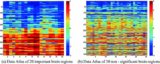
Data Atlas of important and non-vital brain regions with different eye status data
-
(2)
Alzheimer’s disease and normal control data _ Average data map (Line 1 to 140 is Alzheimer’s disease data, Line 141 to 355 is normal data) (Fig. 3).
Fig. 3. 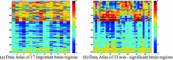
Data Atlas of important and non-vital brain regions with Alzheimer’s disease


We can clearly see from the two sets of data, in the data of the same control group, the distinction in the data of important attributes is greater, and different categories of data are more clearly distinguished. Therefore, the use of important attributes for classification can have a better effect. And the non-important attribute data is usually more disorganized and less distinct, so using it to classify is often ineffective and may even affect judgement.
4.4 Clustering Algorithm Based on Rough Set Optimization
The result of the attribute reduction is taken as an important attribute, and the data that has been subtracted is taken as a non-important attribute. Then the K-means algorithm is used to classify the raw data, the data containing only the important attributes, and the data containing only the non-significant attributes, respectively, where K = 2. The results are as follows (Table 3):
It can be found that, using the important attributes that obtained by the attribute reduction of the rough set to classify, can have a better effect. However, using the non-important attributes that has been subtracted to classify, its accuracy will be less than the raw data, and much less than the important attributes.
5 Discuss
In this paper, a K-means algorithm based on rough set optimization is proposed and applied to the hierarchical fMRI data classification. First, the concepts of important and non-important attributes were put forward. Applicate the rough set theory in the training data set for reduction of attributes, and select the best attribute reduction through the importance of the property. Regard the best attribute reduction of the attribute as an important attribute, the rest attributes as non-important attributes. The important attributes are the most significant cluster of data in the original attributes, and the rest of the attribute often plays a very weak role in the classification, and even affects the classification result. It can be seen from the experiment that the accuracy of classification using the important attributes will be higher than the original data, and the accuracy of the use of non-important attributes of the classification will be lower than the original data, and far below the important attributes. Therefore, the use of important attributes for classification calculation can greatly reduce the workload and can achieve better classification results. In the next step, the experiment can be improved by optimizing the attribute reduction algorithm, selecting the more reasonable strategy of superiority, dividing the more detailed brain region and so on, and obtain the scientific result.
References
Liu, H.B., Abraham, A., Zhang, W.S., Mcloone, S.: A swarm-based rough set approach for fMRI data analysis. Int. J. Innov. Comput. Inf. Control 7, 3121–3132 (2011)
Taylor, M., Donner, E., Pang, E.: fMRI and MEG in the study of typical and atypical cognitive development. Neurophysiol. Clin. 42, 19–25 (2012)
Shad, M.U., Keshavan, M.S.: Neurobiology of insight deficits in Schizophrenia: an fMRI study. Schizophr. Res. 165, 220–226 (2015)
Huang, H., Wang, H.L., Zhou, Y.: Schizophrenia brain resting explore networks and perform network centers and to highlight the relationship between network. Chin. J. Psychiatry 48, 175–181 (2015)
Li, H.J., Hou, X.H., Liu, H.H.: Toward systems neuroscience in mild cognitive impairment and Alzheimer’s disease: a met analysis of 75 fMRI studies. Hum. Brain Mapp. 36, 1217–1232 (2015)
Yang, J.J., Zeng, W.M.: Complex network-based connectivity study in patients with brain function. Chin. J. Med. Imaging 23, 418–422 (2015)
Shi, Y.H., Zeng, W.M., Wang, N.Z., Chen, D.T.L.: A novel fMRI group data analysis method based on data-driven reference extracting from group subjects. Comput. Methods Programs Biomed. 122, 362–371 (2015)
Shi, Y.H., Zeng, W., Wang, N., Zhao, L.: A new method for independent component analysis with priori information based on multi-objective optimization. J. Neurosci. Methods 283, 72–82 (2017)
Pawlak, Z.: Rough set. Int. J. Comput. Inf. Sci. 11, 341–356 (1982)
Wang, G.Y., Yao, Y.Y., Yu, H.: A review of research on rough sets theory and applications. J. Comput. Sci. 1229–1246 (2009)
Zhou, X.Z., Huang, B., Li, H.X., Wei, D.K.: Rough Sets Theory & Approaches for Knowledge Acquisition in Incomplete Information Systems. Nanjing University Press, Nanjing (2010)
Barnali, B., Swarnajyoti, P.: Hyper spectral image analysis using neighborhood rough set and mathematical morphology. In: Accessibility to Digital World (2016). ISBN 978-1-5090-4291
Author information
Authors and Affiliations
Corresponding author
Editor information
Editors and Affiliations
Rights and permissions
Copyright information
© 2017 IFIP International Federation for Information Processing
About this paper
Cite this paper
Li, X., Zeng, W., Shi, Y., Huang, S. (2017). Resting State fMRI Data Classification Method Based on K-means Algorithm Optimized by Rough Set. In: Shi, Z., Goertzel, B., Feng, J. (eds) Intelligence Science I. ICIS 2017. IFIP Advances in Information and Communication Technology, vol 510. Springer, Cham. https://doi.org/10.1007/978-3-319-68121-4_9
Download citation
DOI: https://doi.org/10.1007/978-3-319-68121-4_9
Published:
Publisher Name: Springer, Cham
Print ISBN: 978-3-319-68120-7
Online ISBN: 978-3-319-68121-4
eBook Packages: Computer ScienceComputer Science (R0)