Non-committing Encryption with Constant Ciphertext Expansion from Standard Assumptions

Abstract

Non-committing encryption (NCE) introduced by Canetti et al. (STOC ’96) is a central tool to achieve multi-party computation protocols secure in the adaptive setting. Recently, Yoshida et al. (ASIACRYPT ’19) proposed an NCE scheme based on the hardness of the DDH problem, which has ciphertext expansion $\mathcal {O}(\log \lambda )$ and public-key expansion $\mathcal {O}(\lambda ^2)$.

In this work, we improve their result and propose a methodology to construct an NCE scheme that achieves constant ciphertext expansion. Our methodology can be instantiated from the DDH assumption and the LWE assumption. When instantiated from the LWE assumption, the public-key expansion is $\lambda \cdot \mathsf {poly}(\log \lambda )$. They are the first NCE schemes satisfying constant ciphertext expansion without using iO or common reference strings.

Along the way, we define a weak notion of NCE, which satisfies only weak forms of correctness and security. We show how to amplify such a weak NCE scheme into a full-fledged one using wiretap codes with a new security property.

1 Introduction

1.1 Background

In secure multi-party computation (MPC) protocols, a group of parties can compute some function of their private inputs by communicating with each other. Depending on when corrupted parties are determined, two types of adversarial settings called static and adaptive have been considered for MPC. In the static setting, an adversary is required to declare which parties it corrupts before the protocol starts. On the other hand, in the adaptive setting, an adversary can choose which parties to corrupt on the fly, and thus the corruption pattern can depend on the messages exchanged during the protocol. Security guarantee in the adaptive setting is more desirable than that in the static setting since the former naturally captures adversarial behaviors in the real world while the latter is somewhat artificial.

Beaver and Haber [3] showed if honest parties are assumed to be able to erase sensitive local information completely, then adaptively secure MPC can be obtained efficiently. However, as discussed by Canetti et al. [8], such trusted erasure may be unrealistic in many scenarios.

If private channels are provided between each pair of parties, information-theoretically secure MPC protocols such as those proposed by Ben-Or et al. [7] and Chaum et al. [12] are secure against adaptive adversaries.¹ In order to use those protocols in the actual usage scenarios, we have to simulate private channels by using encryption primitives. For this aim, non-committing encryption (NCE) was introduced by Canetti et al. [8]. Informally, an encryption scheme is said to be non-committing if it can generate a dummy ciphertext that is indistinguishable from real ones but can later be opened to any message by producing a secret key and encryption randomness that “explain” the ciphertext as an encryption of the message. Canetti et al. showed that the information-theoretically secure MPC protocols are still adaptively secure if private channels are replaced by NCE over insecure channels (assumed they are authenticated). Canetti, Lindell, Ostrovsky, and Sahai [9] also showed a slightly augmented version of NCE is useful to achieve adaptive security in the universally composable (UC) setting.

Prior Works on Non-committing Encryption. The ability to open a dummy ciphertext to any message is generally achieved at the price of efficiency. This is in contrast to the ordinary public-key encryption for which we can easily obtain schemes the size of whose ciphertext is by using hybrid encryption methodology, where n is the length of an encrypted message and is the security parameter. Thus, many previous works have focused on constructing efficient NCE schemes. Especially, they tried to improve ciphertext expansion which is the ratio of ciphertext length and message length since ciphertext length dominates the online communication complexity.

In literature, the term NCE was also used to indicate 3-round message transmission protocols which have the non-committing property [2, 15]. In this work, we only focus on 2-round schemes, that is, public-key encryption with the non-committing property.

Canetti et al. [8] constructed the first NCE scheme, based on common-domain trapdoor permutations which can be instantiated from the computational Diffie-Hellman (CDH) or RSA problem. Ciphertext expansion of their scheme is .

Choi, Dachman-Soled, Malkin, and Wee [13] constructed an NCE scheme with ciphertext expansion from trapdoor simulatable PKE. Their construction can be instantiated under many computational problems including factoring problem, since many existing (ordinary) PKE schemes satisfy trapdoor simulatability.

The first NCE scheme with sub-linear ciphertext expansion was proposed by Hemenway, Ostrovsky, and Rosen [23]. They proposed an NCE scheme with ciphertext expansion $\mathcal {O}\!\left( \log n \right)$ for n-bit messages based on the $\varPhi$-hiding problem, which we can easily modify its ciphertext expansion to by dividing long messages to -bit blocks. Hemenway, Ostrovsky, Richelson, and Rosen [22] also showed constructions of NCE with ciphertext expansion from the learning with errors (LWE) and Ring-LWE problems.

Canetti, Poburinnaya, and Raykova [10] studied the construction of NCE in the common reference strings (CRS) model. They achieved optimal ciphertext expansion $1+ o \left( 1 \right)$ assuming the existence of indistinguishability obfuscation (iO) and one-way function.

Recently, Yoshida, Kitagawa, and Tanaka [31] constructed an NCE scheme with ciphertext expansion from a primitive called chameleon encryption (CE), which additionally satisfies oblivious sampleability. They showed an instantiation of obliviously sampleable CE based on the decisional Diffie-Hellman (DDH) problem.

1.2 Our Contribution

We propose the first NCE schemes with constant ciphertext expansion without the use of iO or CRS.

We construct such an NCE scheme based on the construction paradigm using obliviously sampleable CE proposed by Yoshida et al. [31]. Yoshida et al. showed obliviously sampleable CE can be realized based on the DDH problem. In this work, we also show that it can be realized based on the LWE problem for super-polynomially large modulus. As a result, we obtain constant ciphertext expansion NCE schemes based on the DDH problem and LWE problem.

One of the disadvantage of the NCE scheme proposed by Yoshida et al. is its relatively large public-key size. The size of public key for each message bit of their scheme is . In addition to the ciphertext expansion, our LWE based NCE scheme also improves public-key size compared to Yoshida et al.’s scheme. The size of the public key for each message bit of our LWE based scheme is . This is the same as that of NCE scheme proposed by Hemenway et al. [22], which is also based on the LWE problem for super-polynomially large modulus. We provide a comparison between our NCE schemes and existing NCE schemes in Table 1.

Table 1. Comparison of existing (2-round) NCE schemes in terms of their ciphertext and public-key expansion. The security parameter is denoted by . $^{(*)}$ This scheme uses common reference strings.

1.3 Overview

Weak Non-committing Encryption. Our starting point is the observation that by adjusting the parameters of an intermediate version of Yoshida et al. ’s NCE scheme, its ciphertext expansion can be reduced to a constant, at the cost of its perfect form of correctness and security.

Specifically, the scheme only satisfies weak correctness, which means that each bit of decrypted plaintext is flipped with constant probability. Moreover, the scheme only satisfies weak security that only guarantees the secrecy of some part of encrypted plaintexts. In Sect. 3, we formally define weak correctness and weak security for NCE and introduce the notion of weak NCE as NCE satisfying only those weak correctness and weak security.

In Sect. 5, we give the description of the above scheme and its building block, obliviously sampleable CE. Then we prove that the scheme is indeed a weak NCE scheme.

Amplification for Non-committing Encryption. Next, we show that we can amplify a weak NCE scheme into a full-fledged NCE scheme in Sect. 4. As a tool of amplification, we use a coding scheme called wiretap codes. More specifically, we define a new security property, conditional invertibility for wiretap codes. We show an instantiation of wiretap codes constructed from randomness extractor and linear error-correcting codes satisfies the conditional invertibility.

This amplification increases the ciphertext expansion by only a constant factor. Thus, by applying this transformation to the weak NCE scheme shown in Sect. 5, we obtain an NCE scheme with a constant ciphertext expansion.

Lattice-Based Instantiation. We propose a lattice-based instantiation of obliviously sampleable CE in Sect. 6. The construction is a natural composition of the lattice-based hash encryption by Döttling et al. [17] and the lattice-based chameleon hash functions by Cash et al. [11].

One caveat of our construction is that we need the modulus of lattices to be super-polynomially large for the correctness of it. This seems unavoidable since the chameleon encryption implies non-interactive key exchange, which is considered difficult to be realized from lattice problems for polynomially large modulus as discussed by Guo et al. [21].

1.4 Related Works on Amplification for Public-Key Encryption

Studies on security amplification have asked and answered the question: “How far can we weaken a security definition so that schemes satisfying the definition can still be transformed into those satisfying full-fledged security?” Dwork, Naor, and Reingold [18] first studied the amplification of public-key encryption. They showed that a public-key encryption scheme that satisfies weak forms of one-wayness and correctness can be transformed into one satisfies the ordinary correctness and IND-CPA security. Holenstein and Renner [24] showed a more efficient amplification method, starting from a scheme satisfying weak forms of IND-CPA security and correctness. Lin and Tessaro [26] provided an amplification method for schemes with IND-CCA security. In this work, we show an amplification method for NCE, which can be seen as one of this line of research.

2 Preliminaries

Notations. In this paper, PPT denotes probabilistic polynomial time. $x\leftarrow X$ denotes an element x is sampled from uniform distribution over a set X. $y\leftarrow \mathsf {A}(x;r)$ denotes $\mathsf {A}$ given input x, using internal randomness r, outputs y. denotes function f is negligible, that is, holds.

For an integer n, [n] denotes a set $\left\{ 1,\dots ,n \right\}$. For a subset $\mathcal {I}\subset [n]$ and a vector $x=(x_i)_{1\le i\le n}\in \{0,1\}^n$, $x_\mathcal {I}$ denotes $(x_i)_{i\in \mathcal {I}}$. For a matrix $M=(\varvec{m}_i)_{1\le i\le n}\in \{0,1\}^{k\times n}$, $M_\mathcal {I}\in \{0,1\}^{k\times \left|\mathcal {I}\right|}$ denotes the matrix composed from column vectors $\varvec{m}_i$ of M for $i\in \mathcal {I}$.

$h_2(\cdot )$ denotes the binary entropy function, $h_2(p)=-p\log p-(1-p)\log (1-p)$. H(Y|X) denotes the conditional entropy.

Lemma 1 (Chernoff Bound)

Let X be a binomial random variable. If $\mathbb {E}\left[ X \right] \le \mu$, then for all $\delta >0$, $\Pr \left[ X\ge (1+\delta )\mu ) \right] \le e^{-\frac{\delta ^2}{2+\delta }\mu }$ holds.

Lemma 2 (Leftover hash lemma)

Let $\mathcal {H}:=\{h:\{0,1\}^n \rightarrow \{0,1\}^\ell \}$ be a universal hash family. If , (h, h(x)) and (h, u) are statistically indistinguishable where $u\leftarrow \{0,1\}^\ell$.

Channel Model. When a sender transmits a message $x\in \{0,1\}^n$ through a channel $\mathsf {ChR}$, the receiver gets a noisy version of the message $\tilde{x}\in \{0,1,\bot \}^n$. We define the procedure of such channels as probabilistic functions, $\tilde{x}\leftarrow \mathsf {ChR}(x;{r_{\mathsf {ch}}})$. We review two channel models, Binary Erasure Channel (BEC) and Binary Symmetric Channel (BSC).

Let $\mathcal {B}^n_p$ be the n-bit Bernoulli distribution with parameter p. In other words, ${r_{\mathsf {ch}}}\leftarrow \mathcal {B}^n_p$ is an n-bit string where for each $i\in [n]$, $\Pr [{r_{\mathsf {ch}}}_i=1]=p$ and $\Pr [{r_{\mathsf {ch}}}_i=0]=1-p$.

Definition 1

(Binary Erasure Channel (BEC)). Through a binary erasure channel $\mathsf {BEC}_{p}$, each bit of input $x\in \{0,1\}^n$ is erased with probability p.

$\mathsf {BEC}_{p}(x;{r_{\mathsf {ch}}})$ samples randomness ${r_{\mathsf {ch}}}\leftarrow \mathcal {B}^n_p$. Output of the channel is $\tilde{x}$ where $\tilde{x}_i=\bot$ if ${r_{\mathsf {ch}}}_i=1$ and $\tilde{x}_i=x_i$ if ${r_{\mathsf {ch}}}_i=0$.

We also denote the output of BEC by $x_\mathcal {I}\leftarrow \mathsf {BEC}_p(x;{r_{\mathsf {ch}}})$ where $\mathcal {I}=\{i\in [n] \mid {r_{\mathsf {ch}}}_i=0\}$ is the set of non-erased indices.

Definition 2

(Binary Symmetric Channel (BSC)). Through a binary symmetric channel $\mathsf {BSC}_{p}$, each bit of input $x\in \{0,1\}^n$ is flipped with probability p.

$\mathsf {BSC}_{p}$ samples randomness ${r_{\mathsf {ch}}}\leftarrow \mathcal {B}^n_p$. Output of the channel is $\tilde{x}=x\oplus {r_{\mathsf {ch}}}$.

We denote by $\mathsf {BEC}_{\le p}$, a binary symmetric channel with parameter $p'\le p$.

3 (Weak) Non-committing Encryption

A non-committing encryption (NCE) scheme is a public-key encryption (PKE) scheme that has efficient simulator algorithms satisfying the following properties. The simulator can generate a simulated public key $pk$ and a simulated ciphertext $CT$. Later can explain the ciphertext $CT$ as encryption of any message. Concretely, given a message m, can output a pair of randomness for key generation and encryption , as if $pk$ was generated by the key generation algorithm with the randomness , and $CT$ is an encryption of m with the randomness .

Some previous works proposed NCE schemes that are three-round protocols [2, 15]. In this work, we focus on NCE that needs only two rounds, which is also called non-committing public-key encryption, and we use the term NCE to indicate it unless stated otherwise.

In this work, we abstract the intermediate construction of NCE by Yoshida et al. [31] and formalize it as weak NCE. Specifically, we introduce weak correctness and weak security for NCE.

Syntax.  Since an NCE scheme is public-key encryption, we recall its syntax.

Definition 3

(Public-Key Encryption). A PKE scheme consists of the following PPT algorithms .

• : Given the security parameter , using a randomness , it outputs a public key $pk$ and a secret key $sk$.

• : Given a public key $pk$ and a plaintext $m\in \{0,1\}^\mu$, using a randomness , it outputs a ciphertext $CT$.

• : Given a secret key $sk$ and a ciphertext $CT$, it outputs $m$ or $\bot$.

Public-Key/Ciphertext Expansion.  Public-key expansion and ciphertext expansion of a public-key encryption scheme are defined by ${\left|pk\right|}/{\left|m\right|}$ and ${\left|CT\right|}/{\left|m\right|}$, respectively, for .

Correctness.  Since the ordinary correctness can be seen as a special case of weak correctness, we first introduce the notion of weak correctness and then define correctness. Informally, we say that a PKE scheme is weakly correct if it has decryption error for each message bit as defined below.

Definition 4

((Weak) Correctness). We say that a PKE scheme is weakly correct if it has non-negligible decryption error for each plaintext bit. Specifically, we say that $\mathtt {NCE}$ has -decryption error if for all plaintext $m\in \{0,1\}^\mu$ and $i\in [\mu ]$,

holds, where and the probability is taken over the choice of and . In other words, the procedure of encryption and decryption works as the binary symmetric channel

Furthermore, we say that $\mathtt {NCE}$ satisfies correctness if .

Security.  We first introduce the notion of weak security. We then recall the ordinary security of NCE.

Weak security allows an adversary to learn some partial information of a plaintext $\mathsf {Leak}(m)$. Still, it guarantees that other information of m remains hidden. Furthermore, in the security experiment of weak security, the challenge message is fixed in advance independently of the public key.

Definition 5

(Weak Security for NCE). For a PKE scheme and a probabilistic function $\mathsf {Leak}$, consider the following PPT simulators :

• : Given the security parameter , it outputs a simulated public key and its internal state information $st_1$.

• : Given a partial information of a plaintext $\tilde{m}$ which is computed by the probabilistic function $\mathsf {Leak}$ with randomness r, and a state $st_1$, it outputs a simulated ciphertext and a state $st_2$.

• : Given a plaintext m, randomness r used by $\mathsf {Leak}$, and a state $st_2$, it outputs randomness for key generation and encryption .

For an adversary $\mathcal {A}$ and a message m, define two experiments as follows.

We say that $\mathtt {NCE}$ is weakly secure with respect to $\mathsf {Leak}$ if there exist PPT simulators such that for any PPT adversary $\mathcal {A}$ and any message m,

holds.

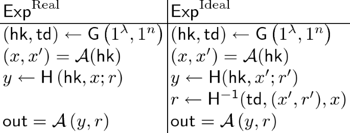
Weak security with respect to $\mathsf {Leak}=\bot$ in which the target message is chosen by the adversary is exactly the same notion as the full-fledged security for NCE which we recall below.

Definition 6

(Security for NCE). For a PKE scheme , consider the following PPT simulators :

• : Given the security parameter , it outputs a simulated public key , a simulated ciphertext and its state $st$.

• : Given a message m and a state $st$, it outputs randomness for key generation and encryption .

For a stateful adversary $\mathcal {A}$, we define two experiments as follows.

We say that $\mathtt {NCE}$ is secure if there exist PPT simulators such that for all PPT adversary $\mathcal {A}$,

holds.

Definition 7

((Weak) Non-Committing Encryption). Let $\mathtt {NCE}$ be a PKE scheme. $\mathtt {NCE}$ is said to be NCE if it satisfies the above correctness and security for NCE. Also, $\mathtt {NCE}$ is said to be weak NCE if it satisfies the above weak correctness and weak security for NCE.

4 Amplification for Non-committing Encryption

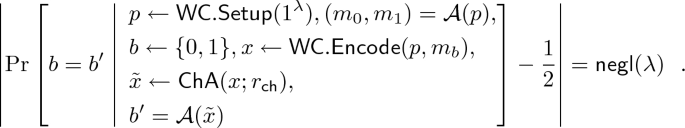
When weak NCE is used to communicate, roughly speaking, the receiver gets a noisy version of the transmitted message x, and the adversary can see some partial information of x. In fact, such a situation is very natural and studied as physical layer security in the Information and Coding (I&C) community since the wiretap channel model was proposed by Wyner [30]. Based on this observation, in this section, we show how to amplify a weak NCE scheme into a full-fledged one by using wiretap codes.²

4.1 Wiretap Codes

As described in Fig. 1, when the sender transmits a message x over the wiretap channel, on one hand, the receiver gets the message affected by noise over receiver channel $\mathsf {ChR}(x)$. On the other hand, an adversary can interrupt the transmission and gets a noisier version of the message $\mathsf {ChA}(x)$.

In such a model, using the difference in the amount of noise the receiver and the adversary are affected, wiretap codes $\mathtt {WC}$ enable us to transmit a message m correctly to the receiver while keeping it information-theoretically secure against the adversary.

Fig. 1.

Wiretap channel model.

Wiretap codes have an encoding and a decoding algorithm similar to error-correcting codes. Wiretap codes satisfy two properties. One is correctness, which ensures that the receiver can decode codewords even if they are affected by some amount of noise. The other is security, which guarantees that the adversary can get no information about the message given some part of the codeword. It is known that the encoding algorithm must use randomness to satisfy security.

Originally in the I&C community, the security of wiretap codes was defined by mutual information. Bellare et al. [4,5,6] proposed several equivalent definitions in a cryptographic manner. Among them, we recall one adopting the distinguishing style of security below. Then we proposed a new security property, conditional invertibility for wiretap codes, which we need in the security proof of our amplification for NCE.

Note that the following definition adopts the seeded version of wiretap codes also proposed by Bellare et al. [6]. In the seeded wiretap channel, the sender, receiver, and an adversary can see a public random seed. We adopt the seeded wiretap codes to give a simple construction of the codes. The seed can be removed without increasing the rate of the codes by a transformation shown in [4]. In this work, we put the seed into a part of the public key when constructing NCE.

Definition 8

(Wiretap Codes). (Seeded) wiretap codes $\mathtt {WC}$ consist of the following PPT algorithms $\left( \mathsf {WC{.}Setup}, \mathsf {WC{.}Encode},\mathsf {WC{.}Decode} \right)$.

• : Given the security parameter , it samples a public seed p.

• : It encodes a message $m\in \{0,1\}^\mu$ with a public seed p and randomness $s\leftarrow \mathbf {S}$, and outputs a codeword $x\in \{0,1\}^n$.

• $\mathsf {WC{.}Decode}(p,x)$: On input a noisy codeword $x\in \{0,1\}^n$ and a public seed p, it outputs a message m.

Rate of Wiretap Codes.  The rate of $\mathtt {WC}$ is the length of messages over the length of codewords $\mu /n\in (0,1)$. The rate of $\mathtt {WC}$ is at most the secrecy capacity of the wiretap channel. The secrecy capacity of wiretap channel, defined with symmetric channels $\mathsf {ChR}$ and $\mathsf {ChA}$, is equal to $H(U|\mathsf {ChA}(U))-H(U|\mathsf {ChR}(U))$ for a uniformly random bit U [25], where H(Y|X) denotes the conditional entropy.

Usually, wiretap codes are required to satisfy the following correctness and security.

As a security property, we present a definition of distinguishing security adopted for seeded wiretap codes. This is a natural extension of the distinguishing security for seedless wiretap codes proposed by Bellare et al. [6].

• Correctness: $\mathtt {WC}$ is correct over the receiver’s channel $\mathsf {ChR}$ if for all message $m\in \{0,1\}^\mu$ and public seed p, we have

  

• Security: $\mathtt {WC}$ is DS-secure against adversary’s channel $\mathsf {ChA}$ if for any unbounded stateful adversary $\mathcal {A}$, we have

  

Next, we introduce a new security property for wiretap codes, conditional invertibility.

Intuitively, this security notion states that after the adversary sees the partial information $\tilde{x}\leftarrow \mathsf {ChA}(x)$ resulted from the codeword x of a message $m'$, we can efficiently explain that $\tilde{x}$ has resulted from another message m. The security definition involves a PPT inversion algorithm $\mathsf {WC{.}Invert}$, which on inputs seed p, a condition $\tilde{x}$, and a message m, outputs randomness $s'$ and ${r_{\mathsf {ch}}}'$ such that $\mathsf {ChA}(\mathsf {WC{.}Encode}(p,m;s');{r_{\mathsf {ch}}}')$ is equal to the condition $\tilde{x}$.

Conditional invertibility implies the ordinary distinguishing security. It can be seen as non-committing security for wiretap codes. Note that wiretap codes are inherently non-committing in the sense that they usually required to statistically lose the information of messages. Thus, the only point conditional invertibility additionally requires is that the inversion can be computed efficiently.

Definition 9

(Conditional Invertibility). For an unbounded stateful adversary $\mathcal {A}$ and a PPT algorithm $\mathsf {WC{.}Invert}$, define two experiments as follows:

We say that $\mathtt {WC}$ is invertible conditioned on $\mathsf {ChA}$ if there exists a PPT inverter $\mathsf {WC{.}Invert}$ such that for any unbounded adversary $\mathcal {A}$,

holds.

4.2 Instantiation of Wiretap Codes

Overview. We recall a modular construction of wiretap codes proposed by Bellare et al. [6] called Invert-then-Encode construction. The building blocks are error-correcting codes and invertible extractors. This idea of composing error-correcting codes and extractors can be found also in the construction of a linear secret sharing scheme proposed by Cramer et al. [14].

Consider an seeded extractor $\mathsf {Ext}:\{0,1\}^k\rightarrow \{0,1\}^\mu$ which on inputs $X\in \{0,1\}^k$ and a seed p, outputs $m\in \{0,1\}^\mu$. The extractor is invertible if there is an efficient inverter $\mathsf {Inv}$, which on inputs $m\in \{0,1\}^\mu$ and seed p, samples a preimage $X\in \{0,1\}^k$ using randomness s. The Invert-then-Encode construction takes input m with seed p, first inverts the extractor $X\leftarrow \mathsf {Inv}(m,p;s)$, then encodes X by the error-correcting code as $x=\mathsf {Encode}(X)$.

For a concrete instantiation, Bellare et al.  suggested to use the polar codes [1] as error-correcting codes to achieve the optimal rate. Note that we can compute the encoding of input m by mG where G is a generator matrix of the linear error-correcting code. Invertible extractors can be instantiated using multiplication over $\mathord {\mathrm {GF}}(2^k)$. Concretely, the extractor takes inputs $x\in \{0,1\}^k$ and seed $p\in \mathord {\mathrm {GF}}(2^k)$, and outputs the first $\mu$ bit of $x\odot p$, where $\odot$ denotes multiplication over $\mathord {\mathrm {GF}}(2^k)$. The inverter $\mathsf {Inv}$ for this extractor is obtained by $\mathsf {Inv}(m,p;s)=(m \Vert s)\odot p^{-1}$.

Construction. We describe the construction of wiretap codes for bit messages. For a longer message, we can encode it by first dividing it into blocks of $\mu$ bit and then encoding each block by the following codes (see [4]).

Let . Let $G\in \{0,1\}^{k \times n}$ be a generator matrix of a linear error-correcting code, and $\mathsf {ECC{.}Decode}$ a corresponding decoding algorithm. Choose a constant $\epsilon >0$ such that the error-correcting code can be correct over $\mathsf {ChR}=\mathsf {BSC}_{\le \epsilon }$. We construct wiretap codes which is correct over $\mathsf {ChR}=\mathsf {BSC}_{\le \epsilon }$ and invertible conditioned on $\mathsf {ChA}=\mathsf {BEC}_{0.5}$. Thus, in this construction, the wiretap decoding algorithm takes as input $x'\leftarrow \mathsf {BSC}_\epsilon (x)$, and the wiretap inverter algorithm takes as input $x_\mathcal {I}\leftarrow \mathsf {BEC}_{0.5}(x;{r_{\mathsf {ch}}})$ where $\mathcal {I}\in [n]$ is the set of non-erased indices determined by a uniformly random n-bit string ${r_{\mathsf {ch}}}$.

• : Sample and output $p\leftarrow \mathord {\mathrm {GF}}(2^k) {\setminus } \{0\}$.

• : For input $m\in \{0,1\}^\mu$, sample $s\leftarrow \{0,1\}^{k-\mu }$, output $x=((m\Vert s)\odot p) G\in \{0,1\}^n$.

• $\mathsf {WC{.}Decode}(p,x')$: Output the first $\mu$ bits of $\mathsf {ECC{.}Decode}(x')\odot p^{-1}$.

• $\mathsf {WC{.}Invert}(p, x_\mathcal {I},m)$: On input a condition $x_\mathcal {I}\leftarrow \mathsf {BEC}_{0.5}(x; {r_{\mathsf {ch}}})$, sample and output $s'$ which satisfies $x_\mathcal {I}=((m\Vert s')\odot p)G_\mathcal {I}$.

  Concretely, let $\sum _i z_i c_i +c_0 (c_i\in \{0,1\}^k,z_i\in \{0,1\})$ be the general solution of linear equation $x_\mathcal {I}=yG_\mathcal {I}$. Then, uniformly sample a solution $\{z_i\}_i$ of linear equation $m=\sum _i z_i(c_i\odot p^{-1})_{\{1,\dots ,\mu \}}+(c_0\odot p^{-1})_{\{1,\dots ,\mu \}}$. Finally, output $s'= \sum _i z_i(c_i\odot p^{-1})_{\{\mu +1,\dots ,k\}}+(c_0\odot p^{-1})_{\{\mu +1,\dots ,k\}}$.

  It also outputs randomness for the channel ${r_{\mathsf {ch}}}'={r_{\mathsf {ch}}}$, which is a uniformly random n-bit string representing the non-erased indices $\mathcal {I}$.

Rate of the Scheme. The rate $\mu /n$ of the scheme can be set to a constant smaller than $(\frac{k}{n}-\frac{1}{2})$. If the rate k/n of the error-correcting codes is close to its capacity $1-h_2(\epsilon )$, the rate of $\mathtt {WC}$ can be close to its secrecy capacity $1/2-h_2(\epsilon )$, which is the optimal rate of wiretap codes.

Correctness. The correctness of the wiretap codes directly follows from the correctness of the underlying error-correcting codes.

Conditional Invertibility. To show the invertibility conditioned on $\mathsf {BEC}_{0.5}$, we need to show that distributions of $(\tilde{x},s,{r_{\mathsf {ch}}})$ are statistically indistinguishable in the real and ideal experiments of the definition. We introduce the hybrid experiment defined as follows:

Claim

The distribution of output in the real and hybrid experiments are same.

Proof

In general, for a function $f:\mathcal {X}\rightarrow \mathcal {Y}$,

$$\begin{aligned} \left\{ (x,y)\mid x\leftarrow \mathcal {X},y=f(x) \right\} \equiv \left\{ (x',y)\mid x\leftarrow \mathcal {X},y=f(x),x'\leftarrow f^{-1}(y) \right\} \end{aligned}$$

holds, where $f^{-1}(y)$ denotes the set of pre-images of y.

By applying the above fact to $f_{p,m}(s,{r_{\mathsf {ch}}})=\mathsf {ChA}(\mathsf {WC{.}Encode}(p,m;s);{r_{\mathsf {ch}}})$, what we need to show is that $\mathsf {WC{.}Invert}$ implements sampling $(s',{r_{\mathsf {ch}}}')\leftarrow f_{p,m}^{-1}(\tilde{x})$.

Since we consider $\mathsf {ChA}=\mathsf {BEC}_{0.5}$, $\mathsf {WC{.}Invert}$ can uniquely determine ${r_{\mathsf {ch}}}'={r_{\mathsf {ch}}}$ from the representation of $\tilde{x}=x_\mathcal {I}$. Recall that $\mathsf {WC{.}Invert}$ samples $s'$ satisfying $x_\mathcal {I}=((m\Vert s')\odot p)G_\mathcal {I}=\mathsf {BEC}_{0.5}(\mathsf {WC{.}Encode}(p,m;s');{r_{\mathsf {ch}}})$ uniformly at random. Hence, the claim follows.    $\square$

Claim

The hybrid and ideal experiments are statistically close if the wiretap codes are secure in the ordinarily sense.

Proof

Consider the adversary $\mathcal {A}$ that distinguished the two experiments. We can construct another adversary $\mathcal {A}'$ against the security of the wiretap codes as follows: Given p, run $\mathcal {A}'$ on p and obtain $m, m'$; send them to its challenger and receive $\tilde{x}$; compute $(s, {r_{\mathsf {ch}}}) \leftarrow \mathsf {WC{.}Invert}(p,\tilde{x},m)$; run $\mathcal {A}'$ on $\tilde{x},s,{r_{\mathsf {ch}}}$ and receive ; output . The claim is proven, since the simulation by $\mathcal {A}$ is perfect.    $\square$

Claim

The wiretap codes are secure in the ordinarily sense.

Bellare et al. [6] show a detailed security proof of the wiretap codes for general $\mathsf {ChA}$. Below, we show a specific security proof for $\mathsf {ChA}=\mathsf {BEC}_{0.5}$.

Proof

Recall that the parameter is selected to satisfy $\mu /n<(k/n-1/2)$. Let $2\delta :=((k-\mu )/n-1/2)>0$ be a constant.

Since $\mathsf {ChA}=\mathsf {BEC}_{0.5}$, the input for the adversary is $x_\mathcal {I}=((m\Vert s)\odot p) G_\mathcal {I}$. By the Chernoff bound, $\left|\mathcal {I}\right|<(\frac{1}{2}+\delta )n$ holds except negligible probability.

Let us decompose the submatrix of the generator $G_\mathcal {I}=PDQ$, where $P\in \{0,1\}^{k\times k}$ and $Q\in \{0,1\}^{\left|\mathcal {I}\right|\times \left|\mathcal {I}\right|}$ are invertible. Furthermore $D=(d_{i,j})\in \{0,1\}^{k\times \left|\mathcal {I}\right|}$ satisfies $d_{i,i}=1$ for $1\le i\le r:=\mathrm {Rank}(G_\mathcal {I})$ and $d_{i,j}=0$ for other elements. We interpret the multiplication by D as getting the first r bits and concatenating $0^{\left|\mathcal {I}\right|-r}$. Thus $x_\mathcal {I}=((((m\Vert s)\odot p)P)_{[r]}\Vert 0^{\left|\mathcal {I}\right|-r})Q$.

For input $m\Vert s$ and seed p, $h_p(m\Vert s):=((m\Vert s\odot p)P)_{[r]}$ forms a universal hash family. Note that the input has min-entropy $\mathbf {H}_{\infty }(m\Vert s)=k-\mu$.

Since holds, by the left over hash lemma, $(p,h_p(m\Vert s))$ is statistically indistinguishable from (p, u) where $u\leftarrow \{0,1\}^r$. Therefore $x_\mathcal {I}$ is statistically indistinguishable from $(u\Vert 0^{\left|\mathcal {I}\right|-r})Q$, which is independent of m. Thus, the claim is proven.    $\square$

By combining the above three claims, conditional invertibility of the wiretap codes follows.

4.3 Full-Fledged NCE from Weak NCE

In this section, we amplify a weak NCE scheme into a full-fledged one using conditionally invertible wiretap codes.

Construction. Let be a weak NCE scheme which has -decryption error and weak security with respect to $\mathsf {BEC}_{0.5}$, and wiretap codes $\mathtt {WC}=(\mathsf {WC{.}Setup},\mathsf {WC{.}Encode},\mathsf {WC{.}Decode})$ which is correct over receiver channel and conditionally invertible against the adversary channel $\mathsf {BEC}_{0.5}$. We construct a full-fledged NCE scheme as follows.

• : 

  • Sample a public seed of the wiretap codes .

  • Generate a key pair of weak NCE .

  • Output $(pk',sk'):=((p,pk),sk)$.

  The randomness for key generation is .

• : 

  • Sample a key for one-time pad $k\leftarrow \{0,1\}^\mu$.³

  • Encode the key as $x\leftarrow \mathsf {WC{.}Encode}(p,k;s)\in \{0,1\}^n$.

  • Compute .

  • Output ciphertext $CT'=(CT, m\oplus k)$.

  The randomness for encryption is .

• : 

  • Parse $CT'$ as $(c_1,c_2)$.

  • Compute .

  • Output $m=c_2 \oplus k$.

Ciphertext Expansion. The ciphertext expansion of $\mathtt {NCE}'$ is

$$\begin{aligned} \frac{\text {ciphertext expansion of }\mathtt {NCE}}{\text {rate of }\mathtt {WC}}+1. \end{aligned}$$

(1)

Since the rate of the wiretap codes is constant, this amplification increases ciphertext expansion only by a constant factor. Combining the ciphertext expansion given in Sect. 5, we will estimate its concrete value for our scheme in Sect. 7.

Correctness.  Due to the decryption error of $\mathtt {NCE}$, each bit of the decrypted codeword x is flipped with probability at most . The wiretap codes correct this error as shown below.

Theorem 1 (Correctness)

If $\mathtt {NCE}$ has -decryption error, and $\mathtt {WC}$ is correct over $\mathsf {BSC}_{\le \epsilon }$, then $\mathtt {NCE}'$ is correct.

Proof

The probability of $\mathtt {NCE}'$ fails to decrypt is evaluated as

Thus $\mathtt {NCE}'$ is correct.

Security.  We now show the security of $\mathtt {NCE}'$.

Theorem 2 (Security)

If $\mathtt {NCE}$ is weakly secure with respect to $\mathsf {BEC}_{0.5}$, and $\mathtt {WC}$ is invertible conditioned on $\mathsf {BEC}_{0.5}$, then $\mathtt {NCE}'$ is secure.

Proof

We first construct a simulator of $\mathtt {NCE}'$ from the simulator of $\mathtt {NCE}$, and the inverter $\mathsf {WC{.}Invert}$ of $\mathtt {WC}$.

•  

  • Sample .

  • Generate .

  • Sample $k\leftarrow \{0,1\}^\mu$.

  • Compute $\tilde{x}\leftarrow \mathsf {BEC}_{0.5}(\mathsf {WC{.}Encode}(p,0^\mu ;s');{r_{\mathsf {ch}}}')$.

  • Compute .

  • Set $pk'=(p,pk), CT'=(CT,k),st'=(st_2,p,k,\tilde{x})$.

  • Output $(pk',CT',st')$.

•  

  • Parse $st'$ as $(st_2,p,k,\tilde{x})$.

  • $(s,{r_{\mathsf {ch}}})\leftarrow \mathsf {WC{.}Invert}(p,\tilde{x},m\oplus k)$.

  • .

  • Output .

Let $\mathcal {A}$ be an adversary against the security of $\mathtt {NCE}'$. We then define the following experiments:

• This experiment is the same as . Specifically,

  • 1. Sample .

  • 2. Generate the key pair .

  • 3. Run the adversary to output plaintext $m\leftarrow \mathcal {A}(p,pk)$.

  • 4. Sample $k\leftarrow \{0,1\}^\mu$ and encoded it as $x\leftarrow \mathsf {WC{.}Encode}(p,k;s)$.

  • 5. Encrypt the codeword as .

  • 6. Output this experiment is .

• In this experiment, we use the simulator for $\mathtt {NCE}$. The ciphertext $CT$ is simulated by only given partial information of the message $\tilde{x}\leftarrow \mathsf {Leak}(x)$, where $\mathsf {Leak}=\mathsf {BEC}_{0.5}$ and $x\leftarrow \mathsf {WC{.}Encode}(p,k;s)$ now. Specifically,

  • 1. Sample .

  • 2. Simulate the public key as .

  • 3. Run the adversary to output plaintext $m\leftarrow \mathcal {A}(p,pk)$.

  • 4. Sample $k\leftarrow \{0,1\}^\mu$ and encoded it as $x\leftarrow \mathsf {WC{.}Encode}(p,k;s)$.

  • 5. Compute partial information $\tilde{x}\leftarrow \mathsf {BEC}_{0.5}(x;{r_{\mathsf {ch}}})$.

  • 6. Simulate the ciphertext as .

  • 7. Explain the randomness for key generation and encryption as .

  • 8. Output of this experiment is .

• In this experiment, we completely eliminate the information of k from the input of to simulate the ciphertext. Later $\mathsf {WC{.}Invert}$ determines the randomness s used in the encode. Specifically,

  • 1. Sample .

  • 2. Simulate the public key as .

  • 3. Run the adversary to output plaintext $m\leftarrow \mathcal {A}(p,pk)$.

  • 4. Sample $k\leftarrow \{0,1\}^\mu$, but the codeword is $x\leftarrow \mathsf {WC{.}Encode}(p,0^\mu ;s')$.

  • 5. Compute partial information $\tilde{x}\leftarrow \mathsf {BEC}_{0.5}(x;{r_{\mathsf {ch}}}')$.

  • 6. Simulate the ciphertext as .

  • 7. Invert the randomness for encode as $(s,{r_{\mathsf {ch}}})\leftarrow \mathsf {WC{.}Invert}(p,\tilde{x},k)$.

  • 8. Explain the randomness for key generation and encryption as .

  • 9. Output of this experiment is .

• In this experiment, we completely eliminate m from the ciphertext by switching k to $m\oplus k$. Specifically,

  • 1. Sample .

  • 2. Simulate the public key as .

  • 3. Run the adversary to output plaintext $m\leftarrow \mathcal {A}(p,pk)$.

  • 4. Sample $k\leftarrow \{0,1\}^\mu$, but the codeword is $x\leftarrow \mathsf {WC{.}Encode}(p,0^\mu ;s')$.

  • 5. Compute partial information $\tilde{x}\leftarrow \mathsf {BEC}_{0.5}(x;{r_{\mathsf {ch}}}')$.

  • 6. Simulate the ciphertext as .

  • 7. Invert the randomness for encoding as $(s,{r_{\mathsf {ch}}})\leftarrow \mathsf {WC{.}Invert}(p,\tilde{x},m\oplus k)$.

  • 8. Explain the randomness for key generation and encryption as .

  • 9. Output of this experiment is .

  Note that the last experiment is identical to .

We show the difference between each experiments are negligible.

Lemma 3

If $\mathtt {NCE}$ is weakly secure with respect to $\mathsf {BEC}_{0.5}$, the difference of in and is negligible.

This lemma directly follows from the weak security of $\mathtt {NCE}$. Note that the message encrypted by $\mathtt {NCE}$ is the key of one-time pad k, which is independent of the public key.

Lemma 4

If $\mathtt {WC}$ is invertible conditioned on $\mathsf {BEC}_{0.5}$, the difference of in and is negligible.

By the conditional invertibility of $\mathtt {WC}$, the following items are statistically indistinguishable.

• $(\mathsf {BEC}_{0.5}(\mathsf {WC{.}Encode}(p,k;s);{r_{\mathsf {ch}}}), (s,{r_{\mathsf {ch}}}))$

• $(\mathsf {BEC}_{0.5}(\mathsf {WC{.}Encode}(p,0^\mu ;s');{r_{\mathsf {ch}}}'), (s,{r_{\mathsf {ch}}}))$ where $(s,{r_{\mathsf {ch}}})$ is output of $\mathsf {WC{.}Invert}( p,\mathsf {BEC}_{0.5}(\mathsf {WC{.}Encode}(p,0^\mu ;s');{r_{\mathsf {ch}}}'),k)$

The lemma follows because , and hence in are computed from the former item, while those in are computed from the latter item.

Lemma 5

  is identical in and .

This lemma holds unconditionally, because $(k, m\oplus k)$ and $(m\oplus k,k)$ distribute identically when k is sampled uniformly at random.

Combining the above lemmas, we complete the proof of Theorem 2.

5 Construction of Weak NCE

In this section, we show an intermediate version of the NCE scheme in Yoshida et al. [31] is a weak NCE scheme. Their scheme is constructed from obliviously sampleable CE. We first recall the definition of obliviously sampleable CE. We then describe the construction of weak NCE, show that it has ${1}/{2^{\ell +1}}$-decryption error, where $\ell$ is a constant which appears in the chameleon encryption, and prove its weak security with respect to $\mathsf {BEC}_{0.5}$. The ciphertext expansion of the resulting weak NCE is $2\ell +o(1)$.

5.1 Obliviously Sampleable Chameleon Encryption

Chameleon encryption (CE) was proposed by Döttling and Garg [16]. We recall its obliviously sampleable variant, introduced by Yoshida et al. [31] as a building block of their NCE scheme. They showed an instantiation of obliviously sampleable CE from the DDH problem. We also show an instantiation from the LWE problem in Sect. 6.

Definition 10

(Obliviously Sampleable Chameleon Encryption). An obliviously sampleable chameleon encryption scheme $\mathtt {CE}$ consists of PPT algorithms for hash functionality , those for encryption functionality , and those for oblivious sampling . We first introduce algorithms for the first two functionality. Below, we let (and , resp.) be the randomness space of (and that of and , resp.). We let $\{0,1\}^\ell$ be the key space.

• : Given the security parameter and the length of inputs to the hash function $1^n$, it outputs a hash key $\mathsf {hk}$ and a trapdoor $\mathsf {td}$.

• : Given a hash key $\mathsf {hk}$ and an input $x\in \{0,1\}^n$, using randomness , it outputs a hash value y.

• : Given a trapdoor $\mathsf {td}$, an input to the hash function x, randomness for the hash function r, and another input to the hash function $x'$, it outputs randomness $r'$.

• : Given a hash key $\mathsf {hk}$, an index $i\in [n], b\in \{0,1\}$, using randomness , it outputs a ciphertext $\mathsf {ct}$.

• : Given a hash key $\mathsf {hk}$, an index $i\in [n], b\in \{0,1\}$, and a hash value y, using randomness , it outputs .

• : Given a hash key $\mathsf {hk}$, a pre-image of the hash function (x, r), and a ciphertext $\mathsf {ct}$, it outputs .

We then introduce algorithms for oblivious sampling.

• : Given the security parameter , it outputs only a hash key $\widehat{\mathsf {hk}}$ without using any randomness other than $\widehat{\mathsf {hk}}$ itself.

• : Given a hash key $\widehat{\mathsf {hk}}$, an index $i\in [n]$, and $b\in \{0,1\}$, it outputs a ciphertext $\widehat{\mathsf {ct}}$ without using any randomness except $\widehat{\mathsf {ct}}$ itself.

An obliviously sampleable CE scheme satisfies the following trapdoor collision property, correctness, oblivious sampleability of hash keys, and security with oblivious sampleability.

• Trapdoor Collision: For a chameleon encryption scheme and a stateful adversary $\mathcal {A}$, we define two experiments as follows.

  

  We say the chameleon encryption scheme satisfies trapdoor collision if for any unbounded stateful adversary $\mathcal {A}$,

  

  holds.

• Correctness: For all , $\mathsf {hk}$ output by either or , we have

  

  where , , and $x_i$ denotes the i-th bit of x.

• Oblivious Sampleability of Hash Keys:  and are computationally indistinguishable.

• Security with Oblivious Sampleability: For any $x\in \{0,1\}^n$, , $i\in [n]$, and PPT adversary $\mathcal {A}$, define two experiments as follows.

  

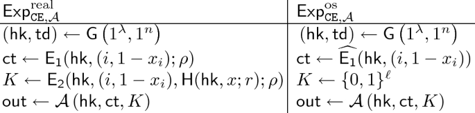
  Then, we have

  

Remark 1

In the original definition of Yoshida et al. [31], security of an obliviously sampleable CE scheme and its oblivious sampleability of ciphertexts are defined separately. In the above definition, we combine them into a single notion, security with oblivious sampleability. This yields a clean and simple security proof of obliviously sampleable CE based on the LWE assumption and that of NCE scheme based on obliviously sampleable CE.

5.2 Construction

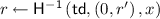
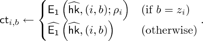
We show a construction of weak NCE scheme $\mathtt {NCE}$ for message space $\{0,1\}^n$ based on an obliviously sampleable CE scheme $\mathtt {CE}$ below. $\mathtt {NCE}$ has constant ciphertext expansion and $\epsilon$-decryption error, and satisfies weak security with respect to $\mathsf {Leak}=\mathsf {BEC}_{0.5}$. We can set $\epsilon$ to be arbitrarily small constant by appropriately selecting the constant parameter $\ell$ of $\mathtt {CE}$; we require that .

• :

  • Generate , and sample $z\leftarrow \{0,1\}^n$.

  • For all $i\in [n]$, sample .

  • For all $i\in [n]$ and $b\in \{0,1\}$, compute

    

  • Output

    

    (2)

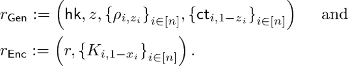
  The key generation randomness is .

• :

  • Parse public key $pk$ as the Eq. 2.

  • Sample randomness and compute .

  • For all $i\in [n]$ and $b\in \{0,1\}$, compute

    

  • Output

    

    (3)

  The encryption randomness is .

• :

  • Parse $sk$ and $CT$ as the Eqs. 2 and 3, respectively.

  • For all $i\in [n]$, compute

    

  • Output x.

Ciphertext Expansion.  Ciphertext length of this scheme is $\left|CT\right|=\left|y\right|+2n\ell$, where length of the output of the chameleon hash $\left|y\right|$ does not depend on n. Therefore ciphertext expansion of this scheme is

$$\begin{aligned} \left|CT\right|/n=2\ell +o(1). \end{aligned}$$

Next, we show that $\mathtt {NCE}$ is weak NCE. More concretely, we show that $\mathtt {NCE}$ has $\epsilon$-decryption error and satisfies weak security with respect to $\mathsf {BEC}_{0.5}$.

Theorem 3 (Weak Correctness)

Let $\ell$ be a constant noticeably larger than $\log (1/\epsilon )-1$. If $\mathtt {CE}$ satisfies correctness, then $\mathtt {NCE}$ has $\epsilon$-decryption error.

Proof

Let $x\in \{0,1\}^n$ be a message encrypted by $\mathtt {NCE}$ and $z\in \{0,1\}^n$ a random string sampled when generating a key pair of $\mathtt {NCE}$.

We fail to decrypt $x_i$ if the underlying chameleon encryption causes correctness error when $z_i = x_i$, or accidentally coincides with when $z_i\ne x_i$. The probability of the former is negligible since $\mathtt {CE}$ is correct, and that of the later is $1/2^\ell$. Notice that correctness of $\mathtt {CE}$ holds for obliviously sampled hash key $\widehat{\mathsf {hk}}$. Thus, the probability of failure to decrypt $x_i$ is evaluated as

   $\square$

Theorem 4 (Weak Security)

If $\mathtt {CE}$ is an obliviously sampleable CE scheme, then $\mathtt {NCE}$ is weakly secure with respect to $\mathsf {Leak}=\mathsf {BEC}_{0.5}$.

Proof

We construct a tuple of simulators as follows.

• :

  • Generate .

  • For all $i\in [n]$ and $b\in \{0,1\}$, compute .

  • Output a simulated public key and state .

• :

  • Sample and compute .

  • For all $i\notin \mathcal {I}$, compute for $b\in \{0,1\}$. For all $i\in \mathcal {I}$, compute

    

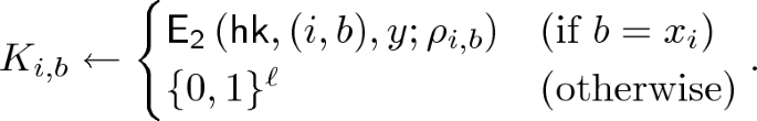
  • Output a simulated ciphertext and state .

• :

  • Sample .

  • Set $z=x\oplus 1^n\oplus {r_{\mathsf {ch}}}$.

  • Output the following simulated randomness

    

Let $\mathcal {A}$ be a PPT adversary against weak security of $\mathtt {NCE}$ and $x\in \{0,1\}^n$. We define the following sequence of experiments.⁴

• : This experiment is exactly the same as . Specifically;

  • 1. Generate and $z\leftarrow \{0,1\}^n$.

  • 2. For all $i\in [n]$, sample .

  • 3. For all $i\in [n]$ and $b\in \{0,1\}$, compute

    

  • 4. Set

    

  • 5. Sample and compute .

  • 6. For all $i\in [n]$ and $b\in \{0,1\}$, compute

    

  • 7. Set

    

  • 8. Output of this experiment is .

• : In this experiment, instead of sampling $z\leftarrow \{0,1\}^n$, we first compute $x_\mathcal {I}\leftarrow \mathsf {BEC}_{0.5}(x;{r_{\mathsf {ch}}})$ and set $z=x\oplus 1^n \oplus {r_{\mathsf {ch}}}$.

Notice that z distributes uniformly at random over $\{0,1\}^n$ also in since ${r_{\mathsf {ch}}}\leftarrow \mathcal {B}^n_{0.5}$. Thus, in is identical to that in . Also notice that $i\in \mathcal {I}$ iff $z_i\ne x_i$ holds by the setting of z.

• : In this experiment, we run instead of .

From the oblivious sampleability of hash keys of $\mathtt {CE}$, the difference of between and is negligible.

In subsequent experiments, we eliminate information of $x_i$ for $i\notin \mathcal {I}$ from the ciphertext .

• : This experiment is defined for $j=0,\dots , n$. is the same experiment as except that we modify the procedures 3 and 6 as follows.

  • 3. For all $i\le j$, compute for .

    For all $i> j$, compute them in the same way as .

  • 6. For all $i\le j$, if $i\notin \mathcal {I}$, compute as and .

    For all $i\le j$, if $i\in \mathcal {I}$, compute them in the same way as .

    Also, for all $i> j$, compute them in the same way as regardless of whether $i\in \mathcal {I}$ or not.

  Note that is exactly the same as .

Lemma 6

If $\mathtt {CE}$ satisfies security with oblivious sampleability, the difference of between and is negligible for every $j\in [n]$.

Proof

Using $\mathcal {A}$, we construct a reduction algorithm $\mathcal {A}^{\prime }$ which attacks the security with oblivious sampleability of $\mathtt {CE}$ with respect to x, r, and j.

What differ in and are $\mathsf {ct}_{i,1-x_i}$, , and .

  is the same in both experiments except negligible probability due to the correctness of CE. We consider the following two cases.

• Case 1. $z_j=x_j$:  $\mathsf {ct}_{j,1-x_j}$ is output of or . is uniform random or output of . In this case, the reduction algorithm $\mathcal {A}^{\prime }$, given , embed $\mathsf {ct}_{i,1-x_i}=\mathsf {ct}^*$, .

• Case 2. $z_j\ne x_j$:  $\mathsf {ct}_{j,1-x_j}$ is output of or .

  is uniform random in both experiments.

  In this case, the reduction algorithm $\mathcal {A}^{\prime }$, given , embed $\mathsf {ct}_{i,1-x_i}=\mathsf {ct}^*$, set .

In both cases, $\mathcal {A}^{\prime }$ returns output .

Depending on $\mathcal {A}^{\prime }$ playing in either $\mathsf {Exp}^{\text {real}}_{\mathtt {CE},\mathcal {A}^{\prime }}$ or $\mathsf {Exp}^{\text {os}}_{\mathtt {CE},\mathcal {A}^{\prime }}$, $\mathcal {A}^{\prime }$ perfectly simulates or except correctness error on , which occurs with negligible probability.

Hence assuming the CE satisfies security with oblivious sampleability, the difference of in and is negligible.

• : This experiment is the same as except that is generated by instead of for every $i\in [n]$.

From the correctness of $\mathtt {CE}$, the difference of between and is negligible.

• : In this experiment, we compute y as , where . Later, we compute r as . Note that this experiment is exactly the same as in which $\mathsf {Leak}=\mathsf {BSC}_{0.5}$ is used. In detail, the experiment proceeds as follows.

  • 1. Generate and $z\leftarrow \{0,1\}^n$.

    For all $i\in [n],b\in \{0,1\}$, compute . Set

    

    Note that this does not depend on z.

  • 2. Compute ,

    

    for all $i\in [n],b\in \{0,1\}$, and

    

    Note that this can be computed only from $x_\mathcal {I}$, where $\mathcal {I}=\{i\in [n] \mid z_i\ne x_i\}$. Moreover, we can regard $x_\mathcal {I}\leftarrow \mathsf {BEC}_{0.5}(x;{r_{\mathsf {ch}}}=x\oplus z\oplus 1^n)$, since $z\leftarrow \{0,1\}^n$ has not appeared elsewhere in this experiment.

  • 3. Sample . Set the randomness as

    

  • 4.

Lemma 7

If the obliviously sampleable CE satisfies trapdoor collision, the difference of in and is negligible.

From the above arguments, we see that $\mathtt {NCE}$ satisfies weak security with respect to $\mathsf {Leak}=\mathsf {BSC}_{0.5}$. This completes the proof of Theorem 4.    $\square$

6 Obliviously Sampleable Chameleon Encryption from Lattices

We propose a lattice-based construction of obliviously sampleable CE. The ciphertext length of the proposed scheme is , which is smaller than of the construction from the DDH problem [31].

The construction is similar to the construction of hash encryption from LWE proposed by Döttling et al. [17]. However we need a super-polynomially large modulus $\mathbb {Z}_q$ for the scheme to satisfy correctness. Although security of the hash encryption is claimed to be proved from a valiant of the LWE assumption, called extended-LWE, we prove the security directly from the LWE assumption.

Before describing our construction, we recall preliminaries on lattices.

6.1 Preliminaries on Lattices

Notations. Let $\varvec{A},\varvec{B}$ be matrices or vectors. $[\varvec{A}|\varvec{B}]$ and $[\varvec{A} ;\varvec{B}]$ denotes concatenation of columns and rows respectively. $\varvec{A}_{\backslash {i}}$ denotes the matrix obtained by removing the i-th column of $\varvec{A}$.

The n-dimensional Gaussian function with parameter s is defined as $\rho _s(\varvec{x}) := \exp (-\pi \Vert \varvec{x}\Vert ^2/s^2)$. For positive real s and countable set A, the discrete Gaussian distribution $D_{A,s}$ is defined by $D_{A,s}(\varvec{x}) = \rho _s(\varvec{x})/\sum _{\varvec{y} \in A} \rho _s(\varvec{y})$. We note that, if $s = \omega (\log {m})$,

$$ \mathop {\Pr }\limits _{\varvec{r} \leftarrow D_{\mathbb {Z}^m,s}}[\Vert \varvec{r}\Vert \le s \sqrt{m}] \ge 1 - 2^{-m+1}. $$

(See [28].)

Parameters. We let , $m=\mathcal {O}\!\left( n\log q \right)$ (e.g., $m = 2 n \log {q}$), . Let $\chi$ be the discrete Gaussian distribution over $\mathbb {Z}$ with parameter $s = \omega (\sqrt{m\log {n}})$, that is, $D_{\mathbb {Z},s}$. Rounding function $\mathsf {round}:\mathbb {Z}_{q}\rightarrow \{0,1\}$ is defined as $\mathsf {round}(v)=\left\lfloor {2v}/{q}\right\rceil$. If input for $\mathsf {round}$ is a vector $\varvec{v}\in \mathbb {Z}_{q}^\ell$, the rounding is applied to each component. $\ell$ be a constant.

Definition 11

((Decisional) Learning with Errors [29]). The LWE assumption with respect to n dimension, m samples, modulus q, and error distribution $\chi$ over $\mathbb {Z}_{q}$ states that for all PPT adversary $\mathcal {A}$, we have

where $\varvec{A}\leftarrow \mathbb {Z}_{q}^{n\times m}, \varvec{S}\leftarrow \mathbb {Z}_{q}^{n\times \ell }, \varvec{E}\leftarrow \chi ^{m\times \ell }, \varvec{B}\leftarrow \mathbb {Z}_{q}^{m\times \ell }$.

Definition 12

(Lattice Trapdoor [19, 27]). There exists following PPT algorithms $\mathsf {TrapGen}$ and $\mathsf {Sample}$.

• Output a matrix $\varvec{A}_T \in \mathbb {Z}_{q}^{n\times m}$ together with its trapdoor $\varvec{T}$.

• $\mathsf {Sample}(\varvec{A}_T,\varvec{T},\varvec{u},s)$: Given a matrix $\varvec{A}_T$ with its trapdoor $\varvec{T}$, a vector $\varvec{u} \in \mathbb {Z}_{q}^n$, and a parameter s, output a vector $\varvec{r} \in \mathbb {Z}^m$.

These algorithms satisfy the following two properties.

• 1. $\varvec{A}_T$ is statistically close to uniform in $\mathbb {Z}_{q}^{n\times m}$.

• 2. If $s \ge \omega (\sqrt{m \cdot \log n})$, then $\varvec{r}\in \mathbb {Z}^{m}$ output by $\mathsf {Sample}(\varvec{A}_T,\varvec{T},\varvec{u},s)$ is statistically close to $D_{\mathbb {Z}^m,s}$ conditioned on $\varvec{r} \in \varLambda _{\varvec{u}}(\varvec{A}_T) := \{\varvec{r}\in \mathbb {Z}^{m} \mid \varvec{A}_T \varvec{r} \equiv \varvec{u} \pmod {q}\}$.

6.2 Construction

We construct an obliviously sampleable CE scheme from the LWE problem for super-polynomially large modulus.

• : 

  • Sample $\varvec{R}\leftarrow \mathbb {Z}_{q}^{n\times N}$ and .

  • Output

    

• : 

  • Sample $\varvec{r}\in \mathbb {Z}_{q}^m$ according to distribution .

  • Output

    $$\begin{aligned} \varvec{y}:=\varvec{A}\cdot [\varvec{x};\varvec{r}] \bmod {q}. \end{aligned}$$

• : 

  • Set $\varvec{y}'= \varvec{R} (\varvec{x} - \varvec{x}')+\varvec{A}_T \varvec{r} \bmod {q}$. Sample and output a short collision by the sampling algorithm of the lattice trapdoor

    $$\begin{aligned} \varvec{r}'\leftarrow \mathsf {Sample}(\varvec{A}_T,\varvec{T},\varvec{y}',s). \end{aligned}$$

• : 

  • Sample where $\varvec{S}\leftarrow \mathbb {Z}_{q}^{n\times \ell }, \varvec{E}\leftarrow \chi ^{\ell \times (N+m)}$.

  • Output

    $$ \mathsf {ct}:={\varvec{S}}^\mathrm {T} \varvec{A}_{\backslash {i}}+ \varvec{E}_{\backslash {i}} \in \mathbb {Z}_{q}^{\ell \times (N+m-1)}. $$

• : 

  • Compute $\varvec{v}={\varvec{S}}^\mathrm {T}(\varvec{y}-b\cdot \varvec{a}_i)+\varvec{e}_i$ and output , where $\varvec{a}_i$ and $\varvec{e}_i$ are the i-th rows of $\varvec{A}$ and $\varvec{E}$.

• : 

  • Compute $\varvec{v}'=\mathsf {ct}\cdot [\varvec{x}_{\backslash {i}};\varvec{r}]$ and output .

• : 

  • Sample and output

    $$\begin{aligned} \widehat{\mathsf {hk}}\leftarrow \mathbb {Z}_{q}^{n\times (N+m)}. \end{aligned}$$

• : 

  • Sample and output

    $$\begin{aligned} \widehat{\mathsf {ct}}\leftarrow {\mathbb {Z}_{q}^{\ell \times (N+m-1)}}. \end{aligned}$$

Trapdoor Collision. For all $\varvec{x},\varvec{x}'$, holds, because the lattice trapdoor samples $\varvec{r}$ such that $\varvec{A}_T \varvec{r}' \equiv \varvec{y}' \pmod {q}$ where $\varvec{y}' = \varvec{R} (\varvec{x} - \varvec{x}')+\varvec{A}_T \varvec{r} \bmod {q}$. Moreover, if $\varvec{r}\leftarrow \chi ^m$, $\varvec{A}_T \varvec{r} \bmod {q}$ is statistically close to uniform over $\mathbb {Z}_{q}^n$ [19, Cor. 5.4], hence $\varvec{y}'$ is also statistically close to uniform. Thus, the distribution of $\varvec{r}'$ is statistically close to $\chi ^m$ (conditioned on $\varvec{R} \varvec{x}' + \varvec{A}_T \varvec{r}' \equiv \varvec{R} \varvec{x} + \varvec{A}_T \varvec{r} \pmod {q}$).

Correctness. Let $\varDelta :=\left|v_j-v'_j\right|$, where $v_j$ and $v'_j$ are the j-th component of the inputs to the rounding function in the computation of and respectively.

$$\begin{aligned} \varDelta&= \left| \left( {\varvec{s}_j}^\mathrm {T} (\varvec{y}-x_i\cdot \varvec{a}_i)+e_{i,j} \right) -\left( \mathsf {ct}_j \cdot [\varvec{x}_{\backslash {i}};\varvec{r}] \right) \right|\\&=\left| {\varvec{s}_j}^\mathrm {T}(\varvec{A}\cdot [\varvec{x};\varvec{r}]-x_i\cdot \varvec{a}_i)+e_{i,j} -\left( {\varvec{s}_j}^\mathrm {T} \varvec{A}_{\backslash {i}}+ \varvec{e}_{\backslash {i,j}} \right) [\varvec{x}_{\backslash {i}};\varvec{r}]\right|\\&=\left|e_{i,j}-\varvec{e}_{\backslash {i,j}}[\varvec{x}_{\backslash {i}};\varvec{r}]\right|\\&\le \Vert \varvec{e}_{j}\Vert \cdot \Vert [\varvec{x};\varvec{r}\Vert \\&\le s\sqrt{N+m} \cdot \sqrt{N+s^2m} \le s^2(N+m), \end{aligned}$$

holds with overwhelming probability. The probability of decryption error on j-th bit is bounded by

which is negligible since the modulus q is super-polynomially large. Thus, by taking the union bound for all $\left|\varvec{v}\right|=\ell$ bits, the probability of decryption error is bounded by

Oblivious Sampleability of Hash Keys. $\varvec{R}$ distributes uniformly at random. The distribution of $\varvec{A}_T$ output by is also statistically close to uniform. Thus, $\varvec{A}$ output by is statistically indistinguishable from the output of .

Security with Oblivious Sampleability. Let $\mathcal {A}$ be an adversary that distinguishes experiments $\mathsf {Exp}^{\text {real}}_{\mathtt {CE},\mathcal {A}}$ and $\mathsf {Exp}^{\text {os}}_{\mathtt {CE},\mathcal {A}}$.

We construct a reduction algorithm $\mathcal {A}^{\prime }$ that breaks the LWE assumption with $(N+m)$ samples by using $\mathcal {A}$ as follows:

• 1. $\mathcal {A}^{\prime }$ receives $\left( \varvec{A}=[\varvec{R}\mid \varvec{A}_T]\in \mathbb {Z}_{q}^{n\times (N+m)},\varvec{B}\in \mathbb {Z}_{q}^{\ell \times (N+m)} \right)$, where $\varvec{B}$ is either ${\varvec{S}}^\mathrm {T}\varvec{A}+\varvec{E}$ or uniformly random.

• 2. $\mathcal {A}^{\prime }$ sets

  $$\begin{aligned} \varvec{a}'&:=(2x_i-1) \left( \varvec{a}_i -\varvec{A}_{\backslash {i}}[\varvec{x}_{\backslash {i}};\varvec{r}] \right) ,\\ \varvec{R}'&:=[\varvec{a}_1\mid \dots \mid \varvec{a}_{i-1}\mid \varvec{a}'\mid \varvec{a}_{i+1}\mid \dots \mid \varvec{a}_{N}]. \end{aligned}$$

  and set

  

• 3. Finally, $\mathcal {A}^{\prime }$ returns .

In the LWE case, that is, $\varvec{B}={\varvec{S}}^\mathrm {T}\varvec{A}+\varvec{E}$ and $\varvec{b}_i = {\varvec{S}}^\mathrm {T}\varvec{a}_i + \varvec{e}_i$, $\mathcal {A}^{\prime }$ statistically simulates $\mathsf {Exp}^{\text {real}}_{\mathtt {CE},\mathcal {A}}$: (1) The distribution of $\mathsf {hk}= [\varvec{R} \mid \varvec{A}_T]$ is the uniform one and statistically close to the real distribution of $\mathsf {hk}$, in which $\varvec{A}_T$ is one of output of ; (2) The distribution of $\mathsf {ct}$ is perfectly correct; (3) The distribution of $K = \mathsf {round}(\varvec{b}_i)$ is also perfectly correct: By our reduction algorithm, we have . Thus, in the computation of , we compute

where we use the fact $(2x_i-1)(2x_i-1)=1$ for $x_i\in \{0,1\}$ to move forth line to fifth line. Therefore, $K = \mathsf {round}(\varvec{v}_i) = \mathsf {round}(\varvec{b}_i)$ has the correct distribution.

In the random case, $\mathcal {A}^{\prime }$ statistically simulates $\mathsf {Exp}^{\text {os}}_{\mathtt {CE},\mathcal {A}}$.

Therefore, assuming the LWE assumption, we obtain .

Public-Key Size of the Resulting NCE. The ciphertext space of this chameleon encryption is $\mathbb {Z}_{q}^{\ell \times (N+m)}$, where , $\ell =\mathcal {O}\!\left( 1 \right)$, , . Thus the length of ciphertexts is

The length of the hash key is

The length of seed for the wiretap codes is . Public key expansion of the resulting NCE scheme is

7 Conclusion

In this work, we constructed NCE schemes with constant ciphertext expansion from the DDH or LWE problem.

Along the way, we defined weak NCE. Given that the full-fledged NCE is a tool to establish private channels in adaptively secure MPC, weak NCE can be interpreted as a tool to establish wiretap channels in adaptively secure MPC. Through wiretap channels, we can securely transmit a message by encoding with wiretap codes that satisfy conditional invertibility.

We showed instantiation of weak NCE that has constant ciphertext expansion and amplified it by using constant rate wiretap codes. Finally, we roughly estimate the ciphertext expansion of the resulting NCE scheme. As we see in Sect. 5, ciphertext expansion of our weak NCE scheme is $2\ell$ asymptotically. Suppose the wiretap codes used in the amplification achieve the secrecy rate $1/2-h_2(\epsilon )$ where $\epsilon =1/2^{\ell +1}$. Then, the ciphertext expansion in Eq. 1 has minimum value $\approx 27$ when $\ell =5$.

We also showed the public-key expansion of our NCE scheme can be reduced to if it is instantiated from the LWE problem. One may think that the use of the ring-LWE problem may further reduce public-key expansion similar to the LWE based NCE scheme by Hemenway et al. [22]. However, unfortunately, it seems that the ring-LWE problem is not helpful to reduce the public-key size asymptotically. Constructing an NCE scheme with constant ciphertext expansion and better public-key expansion is a natural future direction.

References

Arikan, E.: Channel polarization: a method for constructing capacity-achieving codes for symmetric binary-input memoryless channels. IEEE Trans. Inf. Theory 55(7), 3051–3073 (2009)
Beaver, D.: Plug and play encryption. In: Kaliski, B.S. (ed.) CRYPTO 1997. LNCS, vol. 1294, pp. 75–89. Springer, Heidelberg (1997). https://doi.org/10.1007/BFb0052228
Beaver, D., Haber, S.: Cryptographic protocols provably secure against dynamic adversaries. In: Rueppel, R.A. (ed.) EUROCRYPT 1992. LNCS, vol. 658, pp. 307–323. Springer, Heidelberg (1993). https://doi.org/10.1007/3-540-47555-9_26
Bellare, M., Tessaro, S.: Polynomial-time, semantically-secure encryption achieving the secrecy capacity. Cryptology ePrint Archive, Report 2012/022 (2012)
Bellare, M., Tessaro, S., Vardy, A.: A cryptographic treatment of the wiretap channel. Cryptology ePrint Archive, Report 2012/015 (2012)
Bellare, M., Tessaro, S., Vardy, A.: Semantic security for the wiretap channel. In: Safavi-Naini, R., Canetti, R. (eds.) CRYPTO 2012. LNCS, vol. 7417, pp. 294–311. Springer, Heidelberg (2012). https://doi.org/10.1007/978-3-642-32009-5_18
Ben-Or, M., Goldwasser, S., Wigderson, A.: Completeness theorems for non-cryptographic fault-tolerant distributed computation (extended abstract). In: 20th Annual ACM Symposium on Theory of Computing, Chicago, IL, USA, pp. 1–10 (1988)
Canetti, R., Feige, U., Goldreich, O., Naor, M.: Adaptively secure multi-party computation. In: 28th Annual ACM Symposium on Theory of Computing, Philadephia, PA, USA, pp. 639–648 (1996)
Canetti, R., Lindell, Y., Ostrovsky, R., Sahai, A.: Universally composable two-party and multi-party secure computation. In 34th Annual ACM Symposium on Theory of Computing, Montréal, Québec, Canada, pp. 494–503 (2002)
Canetti, R., Poburinnaya, O., Raykova, M.: Optimal-rate non-committing encryption. In: Takagi, T., Peyrin, T. (eds.) ASIACRYPT 2017. LNCS, vol. 10626, pp. 212–241. Springer, Cham (2017). https://doi.org/10.1007/978-3-319-70700-6_8
Cash, D., Hofheinz, D., Kiltz, E., Peikert, C.: Bonsai trees, or how to delegate a lattice basis. In: Gilbert, H. (ed.) EUROCRYPT 2010. LNCS, vol. 6110, pp. 523–552. Springer, Heidelberg (2010). https://doi.org/10.1007/978-3-642-13190-5_27
Chaum, D., Crépeau, C., Damgård, I.: Multiparty unconditionally secure protocols (extended abstract). In: 20th Annual ACM Symposium on Theory of Computing, Chicago, IL, USA, pp. 11–19 (1988)
Choi, S.G., Dachman-Soled, D., Malkin, T., Wee, H.: Improved non-committing encryption with applications to adaptively secure protocols. In: Matsui, M. (ed.) ASIACRYPT 2009. LNCS, vol. 5912, pp. 287–302. Springer, Heidelberg (2009). https://doi.org/10.1007/978-3-642-10366-7_17
Cramer, R., Damgård, I.B., Döttling, N., Fehr, S., Spini, G.: Linear secret sharing schemes from error correcting codes and universal hash functions. In: Oswald, E., Fischlin, M. (eds.) EUROCRYPT 2015. LNCS, vol. 9057, pp. 313–336. Springer, Heidelberg (2015). https://doi.org/10.1007/978-3-662-46803-6_11
Damgård, I., Nielsen, J.B.: Improved non-committing encryption schemes based on a general complexity assumption. In: Bellare, M. (ed.) CRYPTO 2000. LNCS, vol. 1880, pp. 432–450. Springer, Heidelberg (2000). https://doi.org/10.1007/3-540-44598-6_27
Döttling, N., Garg, S.: Identity-based encryption from the Diffie-Hellman assumption. In: Katz, J., Shacham, H. (eds.) CRYPTO 2017. LNCS, vol. 10401, pp. 537–569. Springer, Cham (2017). https://doi.org/10.1007/978-3-319-63688-7_18
Döttling, N., Garg, S., Hajiabadi, M., Masny, D.: New constructions of identity-based and key-dependent message secure encryption schemes. In: Abdalla, M., Dahab, R. (eds.) PKC 2018. LNCS, vol. 10769, pp. 3–31. Springer, Cham (2018). https://doi.org/10.1007/978-3-319-76578-5_1
Dwork, C., Naor, M., Reingold, O.: Immunizing encryption schemes from decryption errors. In: Cachin, C., Camenisch, J.L. (eds.) EUROCRYPT 2004. LNCS, vol. 3027, pp. 342–360. Springer, Heidelberg (2004). https://doi.org/10.1007/978-3-540-24676-3_21
Gentry, C., Peikert, C., Vaikuntanathan, V.: Trapdoors for hard lattices and new cryptographic constructions. In: 40th Annual ACM Symposium on Theory of Computing, Victoria, BC, Canada, pp. 197–206 (2008)
Goldreich, O., Micali, S., Wigderson, A.: How to play any mental game or a completeness theorem for protocols with honest majority. In: 19th Annual ACM Symposium on Theory of Computing, New York City, NY, USA, pp. 218–229 (1987)
Guo, S., Kamath, P., Rosen, A., Sotiraki, K.: Limits on the efficiency of (ring) LWE based non-interactive key exchange. In: Kiayias, A., Kohlweiss, M., Wallden, P., Zikas, V. (eds.) PKC 2020. LNCS, vol. 12110, pp. 374–395. Springer, Cham (2020). https://doi.org/10.1007/978-3-030-45374-9_13
Hemenway, B., Ostrovsky, R., Richelson, S., Rosen, A.: Adaptive security with quasi-optimal rate. In: Kushilevitz, E., Malkin, T. (eds.) TCC 2016. LNCS, vol. 9562, pp. 525–541. Springer, Heidelberg (2016). https://doi.org/10.1007/978-3-662-49096-9_22
Hemenway, B., Ostrovsky, R., Rosen, A.: Non-committing encryption from \(\Phi \)-hiding. In: Dodis, Y., Nielsen, J.B. (eds.) TCC 2015. LNCS, vol. 9014, pp. 591–608. Springer, Heidelberg (2015). https://doi.org/10.1007/978-3-662-46494-6_24
Holenstein, T., Renner, R.: One-way secret-key agreement and applications to circuit polarization and immunization of public-key encryption. In: Shoup, V. (ed.) CRYPTO 2005. LNCS, vol. 3621, pp. 478–493. Springer, Heidelberg (2005). https://doi.org/10.1007/11535218_29
Leung-Yan-Cheong, S.K.: On a special class of wiretap channels (corresp.). IEEE Trans. Inf. Theory 23(5), 625–627 (1977)
Lin, H., Tessaro, S.: Amplification of chosen-ciphertext security. In: Johansson, T., Nguyen, P.Q. (eds.) EUROCRYPT 2013. LNCS, vol. 7881, pp. 503–519. Springer, Heidelberg (2013). https://doi.org/10.1007/978-3-642-38348-9_30
Micciancio, D., Peikert, C.: Trapdoors for lattices: simpler, tighter, faster, smaller. In: Pointcheval, D., Johansson, T. (eds.) EUROCRYPT 2012. LNCS, vol. 7237, pp. 700–718. Springer, Heidelberg (2012). https://doi.org/10.1007/978-3-642-29011-4_41
Micciancio, D., Regev, O.: Worst-case to average-case reductions based on Gaussian measures. SIAM J. Comput. 37(1), 267–302 (2007)
Regev, O.: On lattices, learning with errors, random linear codes, and cryptography. In: 37th Annual ACM Symposium on Theory of Computing, Baltimore, MA, USA, pp. 84–93 (2005)
Wyner, A.D.: The wire-tap channel. Bell Syst. Tech. J. 54(8), 1355–1387 (1975)
Yoshida, Y., Kitagawa, F., Tanaka, K.: Non-committing encryption with quasi-optimal ciphertext-rate based on the DDH problem. In: Galbraith, S.D., Moriai, S. (eds.) ASIACRYPT 2019. LNCS, vol. 11923, pp. 128–158. Springer, Cham (2019). https://doi.org/10.1007/978-3-030-34618-8_5
Acknowledgments
A part of this work was supported by NTT Secure Platform Laboratories, JST OPERA JPMJOP1612, JST CREST JPMJCR14D6, JSPS KAKENHI JP16H01705, JP17H01695, JP19J22363.
Author information
Authors and Affiliations
Corresponding author
Editor information
Editors and Affiliations
Rights and permissions
Copyright information
© 2020 International Association for Cryptologic Research
About this paper
Cite this paper
Yoshida, Y., Kitagawa, F., Xagawa, K., Tanaka, K. (2020). Non-committing Encryption with Constant Ciphertext Expansion from Standard Assumptions. In: Moriai, S., Wang, H. (eds) Advances in Cryptology – ASIACRYPT 2020. ASIACRYPT 2020. Lecture Notes in Computer Science(), vol 12492. Springer, Cham. https://doi.org/10.1007/978-3-030-64834-3_2
Download citation
DOI: https://doi.org/10.1007/978-3-030-64834-3_2
Published:
Publisher Name: Springer, Cham
Print ISBN: 978-3-030-64833-6
Online ISBN: 978-3-030-64834-3
eBook Packages: Computer ScienceComputer Science (R0)