
Abstract
What do we do if our physical system is not perfectly matched to our coordinate system ? This chapter takes a closer look at one aspect of modeling physical systems, namely modeling the most basic robot that has rotational joints. A key concept needed for approaching this and similar problems is coordinate transformation. We focus in particular on mapping Cartesian to spherical coordinates , and vice versa. In addition to refreshing our skills in computing derivatives, special attention must be paid to singularities.
You have full access to this open access chapter, Download chapter PDF
What do we do if our physical system is not perfectly matched to our coordinate system ? This chapter takes a closer look at one aspect of modeling physical systems, namely modeling the most basic robot that has rotational joints. A key concept needed for approaching this and similar problems is coordinate transformation. We focus in particular on mapping Cartesian to spherical coordinates , and vice versa. In addition to refreshing our skills in computing derivatives, special attention must be paid to singularities.
1 Introduction
Because the three dimensions are independent, it is convenient analytically to work with forces in a Cartesian coordinate system. However, robots that actuate a mass in a Cartesian manner would be bigger and more expensive than necessary. In particular, to build a robot that can reach all points in a 1 m × 1 m × 1 m model, we would need machinery that is at least 3 m in length, and that would require substantial space to move. A robot that can rotate and extend needs only to be about 1.73 m long at most; almost half the size. In situations where we have more complex requirements, a multi-link robot can have significant advantages in terms of reach and flexibility, since it can more effectively approximate the shortest feasible path between one point and another. As such, robots with rotational joints and with multiple links have important applications in practice.
To design such robots, we need to have the analytical tools required to model them mathematically. The tools will allow us to determine the location of the links (and joints) at different times, and will also help us to determine the rotational speeds and angular accelerations needed at various joints. One complication to note about the mapping from Cartesian to polar is that there is a singularity (or at least ambiguity) when we are at the origin. This is a technical point that is not so easy to get around, and will require constant attention when we are working with such mappings.
Another key complication to keep in mind is that mapping changes such as speed or acceleration, from Cartesian to polar, depends not only on the magnitude of the change itself but also on the absolute position. Fortunately, this is a complication that can be managed pretty well by using analytical differentiation. In particular, by being careful about independent and dependent variables, and using the chain rule, we can compute closed-form representations of the mapping of changes (or derivatives) from one coordinate system to the other. In doing so, the key analytical skill to keep in mind is looking for patterns in the results of each differentiation step, and to replace any repeating variable by a single variable that we have seen before. This technique of avoiding duplicate expressions keeps derivations manageable and it is rather easy to do. If we skip this step, however, things can easily become complicated.
2 Coordinate Transformation
Let us consider the following illustration, depicting the representation of a point in both Cartesian and polar coordinates :
Using geometry, we know that we can compute the 2D Cartesian representation from the polar one as follows:
This mapping is well-behaved, in that we have a unique value of the Cartesian coordinates for any given value of the polar coordinates. Thus, there are no singularities in this mapping. A singularity is a point where a function is not defined. In general, it is easier to work with functions that have no singularities. A function defined for all possible inputs (of its input type) is called a total function. For example,
is a total function. A function that is not defined for some inputs (of its input type) is called a partial function. For example, g(x) = 1∕x is not defined when x = 0, so, it is a partial function. Note that we refer to the two functions above as one mapping. We can also think of them as one function from pairs to pairs.
We can now compute the derivatives in Cartesian coordinates by differentiating both sides of the equation above. The key thing to note in this case is that we must make extensive use of the chain rule of differentiation, but without being able to simplify it fully.
The chain rule can be expressed in two ways. If we use f and g to represent functions, then we can write it concisely as follows:
A more familiar form might be the following:
or,
Writing it this way helps us see that, if we cannot compute v′ directly, then we can still write a useful expression for it if u′ is a meaningful quantity and we are able to explicitly differentiate v with respect to u. For our example in (6.1) and (6.2), this means that we can differentiate the expressions to obtain the following:
Now we come to the rather important step of looking for patterns in this result, and reducing duplication of expressions as much as possible. This process is important both to help us understand the meaning of the expression that we just computed and also to keep the expression itself small. The latter is especially important if we need to differentiate it again, which is the case, for example, if we eventually want to compute the mapping of accelerations. In our example here, we notice that there are terms corresponding directly to the definition of y and x. Thus, we can simplify the expression for derivatives as follows:
Exercise 6.1 Compute the expression for the second derivative of x and y.
Now we can consider the conversion in the opposite direction, namely going from 2D Cartesian to 2D polar coordinates. We determine the polar coordinates in terms of the Cartesian coordinates as follows:
The first point to note is that this transformation has a singularity. In particular, if l = 0, then the result of the division is not defined.
The second point to note is that, unlike the first one, this transformation is not unique. In particular, there are many other transformations that could give us a result that can be mapped back (by the first transformation ) to the same result. An example would be
or
where K is any integer.
The difficulty introduced by these issues is that we have to carry around with us the requirement that we cannot have l = 0. Other than that, working out how to map the derivatives in Cartesian space back to polar is no different from doing it in the other direction.
Exercise 6.2 Compute the expression for the first and second derivatives of l and θ. The situation is very similar when we go to three dimensions as follows:
The main activity of this chapter’s lab is to demonstrate mastery in deriving the Cartesian to spherical (and vice versa) in a 3D setting, such as the one depicted in Figure 6.1.

3D projections between polar and Cartesian coordinates
The study problems illustrate that the same techniques can be used to convert the local (polar) coordinates of a two-link robot (in 2D) to the global (Cartesian) coordinates.
3 Chapter Highlights
-
1.
From Translational to Rotational Joints
-
(a)
Throughout the project, we have progressed gradually
-
First, we had to determine speeds—this gave us the planning level
-
Second, we determined accelerations (with feedback)—this gave us a simple model of actuation
-
Third, we tuned things to deal with sensing and actuation details
-
Now, we want to figure out how to build an actual robot
-
and that will mean how to work with a single-link robot
We will focus on 2D, but 3D is the subject of the project
-
-
-
(a)
-
2.
From Polar to Cartesian in 2D
-
(a)
Basic equation
-
Using geometry
-
Note that there are no singularities
-
First derivative in detail
-
Second derivative
-
-
(b)
Note about forces and torques
-
(a)
-
3.
From Cartesian to Polar in 2D
-
(a)
Basic equation
-
Still using geometry
-
Note the singularities
-
Derivative of arcsin(x) is \(1/\sqrt {(1-x^2)}\)
-
-
(b)
Beyond a single-link
-
A two-link example
-
Defining positions equations using geometry
-
Inversion gets more complicated
-
Calculating derivatives
-
-
(a)
4 Study Problems
This study problem focuses on practicing basic analytical differentiation.
-
1.
Assume that a, b, x, y are dependent variables that vary as a function of the independent variable t. Consider further the following relations:
\(a\ = \sqrt {x^2\ + \ \sin {}(y/x)}\),
\(b\ = \ a\ + \ x*y/(\sin {}(a))\).
Assume further that the notation x′ means dx∕dt. Compute the following values:
-
(a)
da∕dt in terms x, x′, y, and y′.
-
(b)
db∕dt in terms of a, a′, x, x′, y, y′.
Show all your intermediate work. You may use notation “del a/ del b” for the partial derivative of “a” with respect to “b.”
-
(a)
-
2.
Consider the simple two-link system shown in Figure 6.2.
Fig. 6.2 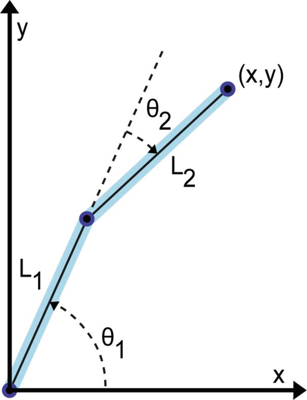
A simple two-link system
-
(a)
Write the formula for (x, y) in terms of the other variables in the diagram.
-
(b)
Assuming ALL variables can change with time, write down the formula for the first derivative of x and the first derivative of y.
-
(c)
Assuming that ONLY the length variables (not the angle variables) can change, write down the equations for the second derivative of x and the second derivative of y.
-
(a)
-
3.
Consider the mechanism in Figure 6.3
-
(a)
Assume that the length of the first link is L, and that the length of the second link is L. Assume further that the end of the second arm is a point at (x, y) with respect to the coordinate system (x 0, y 0). Write an expression for the value of x and y in terms of L, θ 1, and θ 2.
-
(b)
Write an expression for the derivative of x in terms of θ 1 and θ 2. Do the same for y.
Fig. 6.3 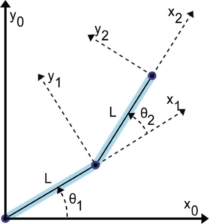
A two-link mechanism
-
(a)
-
4.
Consider the triple-pendulum mechanism shown in Figure 6.4
Fig. 6.4 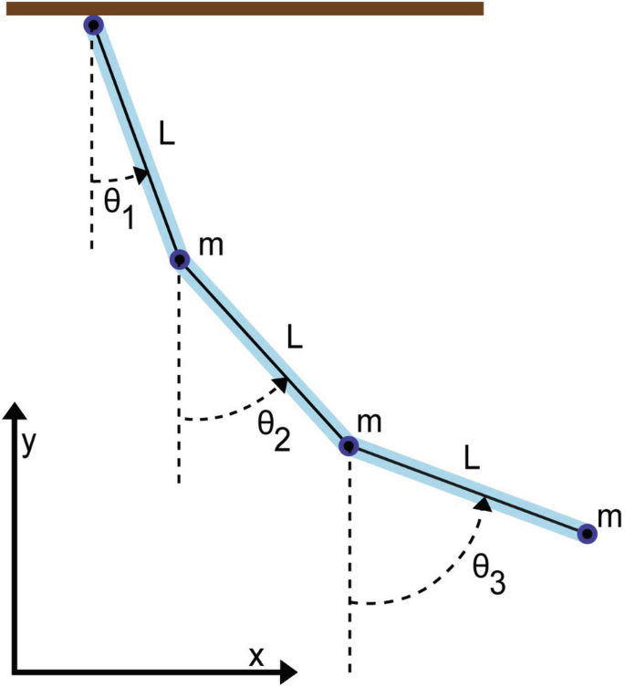
A triple-pendulum mechanism
-
(a)
Assume that the x axis points to the right, the y axis points up, and the origin is at the bottom of the diagram (the exact position is irrelevant for this problem). Assume the first point from the base is at (x 1, y 1), the second is at (x 2, y 2), and the third is at (x 3, y 3). Write the expression for (x 3, y 3) in terms of θ 1, θ 2, θ 3, and l. Your answer should not expand x 1, y 1, x 2, and y 2.
-
(b)
Write an expression for the second derivative of y 3 in terms of θ 1, θ 2, θ 3, and l.
-
(a)
-
5.
Consider the mechanism shown in Figure 6.5:
Fig. 6.5 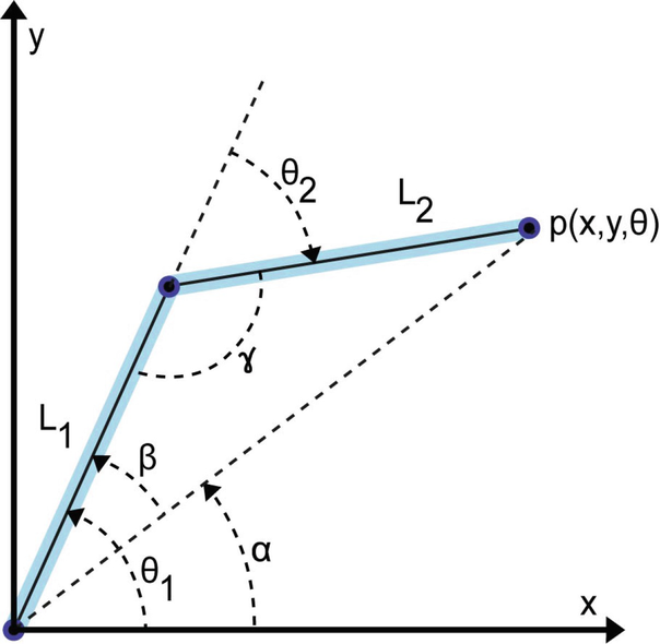
A two-link mechanism
The positive x axis points to the right, the positive y axis points up, and the origin is at the bottom left of the diagram.
-
(a)
Write the expression for x and y for point p(x, y, θ) in terms of θ 1, θ 2, l 1, and l 2.
-
(b)
Let l 3 be the distance of point p(x, y, θ) from the origin. Write an expression for the α and l 3 in terms of x and y.
-
(c)
Write an expression for the second derivative of both x and y in terms of the other variables and their derivatives. Make sure that your answer provides equations that clearly define these values in terms of θ 1, θ 2, l 1, and l 2 and/or their derivatives.
-
(a)
-
6.
Go back to the first assignment and consider your explanation of the challenges. Write a single page containing the following:
-
(a)
Your original submission from the first assignment, with title Original Submission. This part should be at most one page.
-
(b)
A first revision of this submission is based on what you know now. In this revision, your goal is to simply say what you were trying to say at the beginning of the semester, but to say it more clearly using the concepts that you now know. For example, do not add any new challenges. This revision is also a good opportunity to use proper terminology that you may have not been familiar with at the start of the book. This part should be at most one page.
-
(c)
Based on this first revision, make a second one that explains what you see as the most important challenges from your point of view now. In addition, it should explain how you would go about building such a robot. This part can be up to two pages.
-
(a)


5 Lab: Coordinate Transformations
The purpose of this lab is to connect the theoretical discussion of coordinate transformation already seen in this chapter with the concrete use in the context of a simulation of a particular control problem.
Let us consider a situation where there is a ball being moved in a circular orbit with a single-arm robot. There are only two degrees of freedom: The angle around the center of motion and the length (extension of the arm). This can be represented using the following model:

To facilitate visualization in this example, we have also used the _3D mechanism for generating animations. As we add more objects you should also extend that statement to visualize those objects as well.
Note that here we chose to give the red ball the dynamics of having a constant angular velocity theta' but a fluctuating radial speed l'. This makes it move in an almost-but-not-quite circular orbit.
Simulate the model to confirm that it behaves as described. Inspect the plots to familiarize yourself with the behavior of the different variables involved.
Now imagine that we would like to build a controller for a robot arm that should follow this path. There are in general many choices for how to do this, but imagine that we have to build to separate controllers, one for the angle of the arm and one for the extension of the arm. This means that the angular actuation can only depend on angles and the extension actuation can only depend on extensions. For simplicity, we decide to use PID control. The following controller can be modeled as follows:

Simulate this model to confirm that it behaves as described. Note that the performance of the controller can be improved by tuning the gains, but for our purposes smaller gains make it easier to have a distance between the two balls, and to remember which one is which.
Now imagine a situation where our robot was upgraded, and the new robot was Cartesian rather that polar. That is, the new robot consisted of two orthogonal belts, one moved an entire platform in the x direction, and another sitting on this platform could be moved in the y direction. The new robot is also more computationally powerful, so, it can calculate trigonometric functions quickly. Our new task is now to calculate the control signals that the controller for the new robot needs to generate so that it acts exactly as the old controller did. In other words, we have to transform all of our signals from polar to Cartesian.
Use the methods that you have learned about in this chapter to convert the above signals for the green ball to signals in polar coordinates. First do this using pen and paper and then map it back to the model. To make room for it in the model, introduce a new object consisting of a blue box as follows:


When you have calculated the new controller signals, insert in place of the zero on the lines that say Fix me. The formulae that you insert may use all variables of the green ball and the blue cube, but should not make any direct reference to the red ball.
When you are done, simulate your model. If your answer is correct, your blue cube will coincide exactly at all times with the green ball. This should confirm to you that you have successfully mapped the acceleration signals for the green ball into equivalent acceleration signals for the blue ball.
6 Project: Spherical-Actuation for Ping Pong Robot
So far in the project we worked in Cartesian space rather than the space that is most natural with respect to how the components of our robot player move. To remove this simplifying assumption, your task in this project’s activity is to convert the accelerations computed by the controller that you built in the previous activity into forces and torques for the single-arm robot that we are working with. The conventions for the coordinate transformation used for this stage of the tournament are represented by the following diagram:

Develop the mathematical equations for this transformation so that you produce the correct actuation signals to your robot. Your change should be made in the player model, and specifically where it says:
// You need calculate the following equations according // to correct coordinate transformation //r'' = 0 // Wrong value!!! //Alpha'' = 0 // Wrong value!!! //theta'' = 0 // Wrong value!!!
As part of this activity, you should reflect on how you derived the correct coordinate transformation. Consider whether you think it was useful to ignore these effects initially or if it would have been better to include them from the outset. You can use your old path planning strategies developed for tournament 1 and 2. Also, since this is a project, it is useful to reflect on how you developed your player and what you learned from this experience.
7 To Probe Further
-
Articles on Polar (2D) and Spherical coordinate (3D) systems
-
Video about a boy that gets a 3D-printed prosthetic hand
-
Video about a multi-link robot
Author information
Authors and Affiliations
Rights and permissions
Open Access This chapter is licensed under the terms of the Creative Commons Attribution 4.0 International License (http://creativecommons.org/licenses/by/4.0/), which permits use, sharing, adaptation, distribution and reproduction in any medium or format, as long as you give appropriate credit to the original author(s) and the source, provide a link to the Creative Commons license and indicate if changes were made.
The images or other third party material in this chapter are included in the chapter's Creative Commons license, unless indicated otherwise in a credit line to the material. If material is not included in the chapter's Creative Commons license and your intended use is not permitted by statutory regulation or exceeds the permitted use, you will need to obtain permission directly from the copyright holder.
Copyright information
© 2021 The Author(s)
About this chapter

Cite this chapter
Taha, W.M., Taha, AE.M., Thunberg, J. (2021). Coordinate Transformation (Robot Arm). In: Cyber-Physical Systems: A Model-Based Approach. Springer, Cham. https://doi.org/10.1007/978-3-030-36071-9_6
Download citation
DOI: https://doi.org/10.1007/978-3-030-36071-9_6
Published:
Publisher Name: Springer, Cham
Print ISBN: 978-3-030-36070-2
Online ISBN: 978-3-030-36071-9
eBook Packages: Computer ScienceComputer Science (R0)