Encapsulation and Sharing in Dynamic Software Architectures: The Hypercell Framework

Abstract

We present in this paper a novel framework for the definition of formal software component models, called the Hypercell framework. Models in this framework (hypercell models) allow the definition of dynamic software architectures featuring shared components, and different forms of encapsulation policies. Encapsulation policies in an hypercell model are enforced by means of runtime checks that prevent a component, in a given context, to evolve in violation of these policies. We present the main elements of the framework, its operational semantics and the first elements of its behavioral theory. We give some results concerning its ability to express different forms of composition, and show by means of examples its ability to deal with sharing and different forms of encapsulation.

1 Introduction

Motivations. How do we formally model dynamic software architectures featuring both encapsulation and sharing? Can we define an operational semantics and behavioral theory for these architectures? These are the questions we deal with in this paper. By dynamic software architectures, we understand structured collections of software components and their inter-relations [3], that can evolve over time, either spontaneously, for instance to adapt to changing operating conditions, or following external intervention, for instance for purposes of fault correction or functional update. By encapsulation, we understand forms of confinement and isolation between components, typically coupled with information hiding and abstraction, that ensure capabilities offered, and information maintained by a component, can only be accessed through designated interaction points or interfaces. Examples include the many forms of encapsulation that have been studied under the topic of aliasing control and ownership types in object-oriented programming [14]. By architectures with sharing, we understand architectures where components can take part in different ensembles, compositions or aggregations, possibly with different attendant properties, e.g. in terms of encapsulation, lifetime and existential dependencies [2]. Examples include architectures featuring common services, such as databases or logs, that can be used by software components at different levels in a software structure, and architectures featuring shared resources such as virtual machines or operating system processes.

Fig. 1.

Architecture with sharing: shared log service

An example can illustrate the questions we are concerned with. Consider the architecture depicted in Fig. 1. In the figure, a composite component C has two subcomponents, $C_1$ and $C_2$, equipped with private log subcomponents $L_1$ and $L_2$, that are provided as client-specific logs by a composite log service component L (in the picture, components are depicted as circles, and an arrow from component X to component Y can be read as X contains Y, or Y is a subcomponent of X). The log service $L$ is shared among the two subcomponents $C_1$ and $C_2$. One can argue that each private log component $L_i$ ($i=1,2$) is participating to three different ensembles, $C_i$, C and L. $C_i$, because $L_i$ is existentially dependent on $C_i$, and is partially encapsulated in $C_i$ as only updates originating from $C_i$ are possible (it is a partial encapsulation because not all communication between a component $L_i$ and its environment is mediated or controlled by $C_i$). C because each $C_i$ is a subcomponent of C, and C is supposed to encapsulate its subcomponents. L, because $L_i$ is existentially dependent on L, has the same lifetime as L (if L is deleted so are $L_1$ and $L_2$), and relies on private functions (e.g. data storage) provided by L. These ensembles also correspond to encapsulation scopes, whose meaning is, roughly, that no communication outside the scope is possible without explicitly passing through the top component of each scope ($C,L,C_1$ or $C_2$), except for the communications between $C_i$ and $L_i$.

Related Work. Over the past three decades, an abundant literature has developed that aims at formally modeling distributed, component-based, dynamic and adaptive software architectures, systems and services. One can cite notably: process calculi for distributed systems, such as $\pi$-calculi with localities [12, 22, 31], Ambient Calculi and their variants [10, 11], and Milner’s bigraphs [28, 35]; process calculi and formal models for service-oriented computing and adaptive systems [9, 17, 19, 20, 37]; formal software component models such as BIP [6], Ptolemy [18], Reo [23], Community [40], and several others [24, 25]; formal software architecture description languages [26, 32]. However, to the best of our knowledge, none of these previous works provide satisfactory support to model architectures featuring a combination of dynamicity, sharing and encapsulation. Synchronized Hyperedge Replacement (SHR) systems and location graphs constitute a direct inspiration for the work in this paper, but they do not allow the definition of encapsulation scopes with sharing. Ownership types allow the enforcement of encapsulation scopes in object-oriented programs, typically at the expense of restrictions in inter-object communication, but do not allow overlapping encapsulation scopes. Bigraphs with sharing [35] support the definition of nodes with overlapping containment scopes, but, as far as we are aware, it is not possible to use bigraph nodes to enforce the encapsulation policies considered in this paper. The Fractal component model [8] is one of the rare software component models that allows the description of component configurations with sharing, and that has been formally defined [27]. The architecture in Fig. 1 can readily be described in Fractal, with encapsulation scopes captured by Fractal composites. But we do not have a formal operational semantics for Fractal that would allow us to define the exact semantics of these scopes, nor do we have a proper behavioral theory for Fractal architectures. Interesting approaches to enforcing encapsulation policies are works that rely on dynamic access protection instead of aliasing control. These include notably the Siaam actor abstract machine [15], which relies on runtime checks to enforce actor encapsulation in a Java virtual machine, and access contracts [39] which provide dynamic access protection to Java objects that can support a wide range of encapsulation policies, including encapsulation policies with sharing as in the small architecture depicted in Fig. 1. However, Siaam and access contracts do not come with a formal behavioral theory, and the question of program equivalence in concurrent languages with Siaam-like or access contracts-like access protection mechanisms remains open.

Contributions. In this paper, we combine ideas from SHR systems [19], from location graphs [36], as well as Siaam [15] and access contracts [39] dynamic approaches to encapsulation enforcement, to define a formal operational framework, called the Hypercell framework. This framework allows the definition of different software component models (hypercell models), that support the modelling of dynamic component ensembles (hypercells) with sharing and encapsulation. The Hypercell framework can be seen as a conservative extension and generalization of the BIP and Fractal components models [6, 8]. A main contribution of the Hypercell framework is how it handles encapsulation policies: to allow for maximum flexibility, they are enforced by runtime checks (authorizations), that prevent transitions of component ensembles that would violate the chosen policies. Defining a proper notion of authorization is not trivial however. In order to obtain a proper component theory (e.g. in the sense of [4]), we need a notion of hypercell equivalence that is a congruence for hypercell composition, and it is not clear how such a result can be obtained in presence of authorizations. The idea is to have authorizations operate only at the level of individual components (cells): this allows us to define a notion of hypercell bisimilarity where we can decouple the contribution of authorizations from the classical bisimulation game, which in turn allows us to obtain the required congruence result. However, this local form of authorization raises another problem: encapsulation policies are not local in nature, so how can we enforce them via such local checks, notably in presence of evolving component ensembles? We show, by means of examples, how this can be done via a combination of local but context-dependent authorization predicates and dynamic component types (cell sorts).

Outline. The paper is organized as follows. Section 2 is a brief informal introduction to hypercells. Section 3 presents the hypercell framework, and preliminary elements of a behavioral theory for hypercell models. Section 4 shows, by means of examples, how to enforce different forms of encapsulation using sorts and authorizations. Section 5 concludes the paper.

2 Informal Introduction

A hypercell is a finite set of cells. A cell has (we also say “offers”) roles (a term we borrow from location graphs). A role is a point of attachment for cells, as well as a point of interaction between cells. A hypercell, much like a SHR system, constitutes a hypergraph, where the roles are vertices, and cells are the edges of the hypergraph. A role corresponds to a point of attachment and interaction between cells, and may be offered at most by two distinct cells. Hypercells are thus limited forms of hypergraphs, where hyperedges can connect any number of vertices, but a given vertex can only be connected by at most two edges. As in standard software component model ontology [16], roles are classified as provided or required: a provided role in a cell signals some service offered by the cell, whereas a required role signals some expected service. When a role belongs to two cells in a given hypercell (in required position in one cell, and in provided position in the other cell), we say that the role is bound, and that it binds the two cells that offer it. Otherwise, we say that the role is unbound.

A cell is a locus of computation, as are localities in process calculi such as the Distributed $\pi$-calculus [31], and Klaim [29]. One can understand a cell as a basic software component or as a connector, as in the component-and-connector view of software architecture [3] and in software component models [16]. A hypercell can be understood as a composite software component or component ensemble. In this sense, the hypercell concepts align well with the standard concepts of software component models [16] and software architecture, as present e.g. in the ACME [21] and Fractal [8] component models (cells and hypercells correspond to ACME and Fractal components, roles to ACME ports and Fractal interfaces, bound roles to Fractal primitive bindings).

Figure 1 depicts a small hypercell with roles drawn as black dots (or arrows when bound) and cells as ellipses. Interactions in a hypercell take the form of simple point-to-point bidirectional interactions between pairs of cells bound by some role. In Fig. 1, cells $C_1$ and $L_1$ can interact directly because they are bound, but $C_2$ cannot directly interact with $C_1$, nor C with L. In the architecture depicted in Fig. 1, the scopes discussed in the introduction are manifested by bound roles and the sorts adorning the different cells (hinted at by arrows).

The behavior of a hypercell is the result of the composition of the behavior of its cells. A cell evolves by transforming into some hypercell, in the process possibly interacting with, or removing, cells it is bound to. The evolution of a hypercell corresponds to the parallel firing of a number of such cell transitions. An interaction between two cells bound at a role r amounts to several binary rendez-vous on communication channels succeeding at role r. An interaction will typically result in the simultaneous exchange of values at each of the channels participating in the interaction.

For instance, a client-server interaction at role r between a client cell C and a server cell S, may, on the server side, take the form $\overline{r}: \{ \mathtt {op}\langle v,\mathtt {resp} \rangle , \overline{\mathtt {resp}}\langle w \rangle \}$, where r is the role which appears in provided position in the server (hence the overline $\overline{r}$), $\mathtt {op}$ is the channel on which the value v is sent, along with the return channel $\mathtt {resp}$, and w is the value which is (instantly) returned by the server, in response to the request $\mathtt {op}\langle v,\mathtt {resp} \rangle$, on the requested return channel $\mathtt {resp}$. On the client side, the interaction would take the conjugate form $r: \{ \overline{\mathtt {op}}\langle v,\mathtt {resp} \rangle , \mathtt {resp}\langle w \rangle \}$. Notice that we use an early form for interactions: this allows us, in the operational semantics of hypercell models, to abstract from syntactic details such as a distinction between sent values and receiving parameters (the latter typically under the scope of some binding constructs). Our operational semantics thus has no mention of substitution of values to formal parameters, but we do distinguish with channels between originating side (e.g. $\overline{\mathtt {op}}$, on the client side) and receiving side (e.g. $\mathtt {op}$, on the server side).

Interactions between cells can be higher-order. In particular cells can be exchanged as values on channels during interactions. This allows the removal or passivation of cells as in the Kell calculus [34], which in turns allows to model objective reconfigurations in software architectures, where certain components can exercize explicit control over other ones.

Interactions between bound cells in a hypercell can be guarded by priorities. Priorities are crucial for the expressive power of the framework and the definition of different forms of composition operators as cells or hypercells. A priority allows a cell to check for the presence or absence of a signal from another cell it is bound to, in the form of the ability or inability to communicate on a given channel. For instance the client side communication above could be guarded by the absence of communication on channel $\mathtt {sig}$ on role s, which we would write thus: $\langle \{ s: \lnot \overline{\mathtt {sig}} \} \cdot \overline{r}: \{ \mathtt {op}\langle v,\mathtt {resp} \rangle , \overline{\mathtt {resp}}\langle w \rangle \} \rangle$. In effect, the possible emission of signal $\mathtt {sig}$ on role s preempts (takes priority over) the emission of the request $\mathtt {op}$ on role r.

Individual cell transitions are also guarded by authorizations. An authorization is a runtime check that determines whether a cell transition is licit or not. Authorizations rely on the hypercell context of an individual cell to make this determination. For instance, a cell within an encapsulation scope can be prevented from making a transition that would allow it to bind to a cell outside this scope, whereas the same transition of the cell outside of such a scope can be allowed to proceed.

3 The Hypercell Framework

We define in this section our Hypercell framework. This framework can be instantiated to yield different hypercell models. Each hypercell model must define the following sets: a set of processes; a set of sorts; an infinite set of roles; a set of values; an infinite set of names; an infinite set of channels; a set of unconstrained transitions; and an authorization predicate $\mathtt {Auth}$. We require , , and that the sets , , and be mutually disjoint. Values can comprise processes, sorts, and names as well as elements of other datatypes (booleans, integers, etc). Values can be exchanged between cells on channels at bound roles. We require that the set contain the special channel $\mathtt {rmv}$, which is used in hypercell models with objective cell removal. We require the set of names to be equipped with an involution, called the conjugate operation, which sends a name a to its conjugate $\overline{a}$. By definition, we have $\overline{\overline{a}} = a$, and we write $\widehat{a}$ to denote a or its conjugate $\overline{a}$.

We require that each of the sets above be equipped with an operation for swapping names: for any element x of the above sets, $(r \; s) \cdot x$ yields an element of the same set where names r and s have been permuted, i.e. where r is replaced by s. (in the long version of this paper, we require the datatypes above to be nominal sets [30], but for lack of space we do not go into details here). We also require the existence of an operation $\mathtt {supp}$ that extracts from an element the set of names it contains, and we write $a \#X$ for $a \not \in \mathtt {supp}(X)$.

Formally, a cell in a hypercell model is a 4-tuple of the form $[P:\mathfrak {s} \; \triangleleft \; \mathbf {p} \, \bullet \, \mathbf {r}]$, where P is the process of the cell, $\mathfrak {s}$ is the sort of the cell, $\mathbf {p}$ and $\mathbf {r}$ are the sets of provided and required roles of the cell, respectively. If $C = [P:\mathfrak {s} \; \triangleleft \; \mathbf {p} \, \bullet \, \mathbf {r}]$, we have $C.\mathtt {process}= P$, $C.\mathtt {sort}= \mathfrak {s}$, $C.\mathtt {prov}= \mathbf {p}$, and $C.\mathtt {req}= \mathbf {r}$. Any cell C must meet the following constraints: $C.\mathtt {prov}\cap C.\mathtt {req}= \emptyset$. The set of cells in a hypercell model is noted . The process of a cell embodies its behavior; the fact that a process can be a value means that cells can potentially update their behavior dynamically. The sort of a cell is a dynamic type associated with the cell; sorts are used to enforce runtime constraints on cells, as is shown in Sect. 4.

A hypercell G is just a set of cells that meets the following constraints: for any partition $G_1,G_2$ of G ($G = G_1 \cup G_2$ and $G_1 \cap G_2 = \emptyset$), one must have $G_1.\mathtt {prov}\,\cap \, G_2.\mathtt {prov}= \emptyset$ and $G_1.\mathtt {req}\,\cap \, G_2.\mathtt {req}= \emptyset$, where the set $G.\mathtt {prov}$ of provided roles of hypercell G is defined as $\bigcup _{C \in G} C.\mathtt {prov}$ (and likewise for the set $G.\mathtt {req}$ of required roles of G). We note $\mathsf {0}$ the empty hypercell, and the set of hypercells in a hypercell model. We define the set of roles, of bound roles and unbound roles of a hypercell G:

When G and $G'$ are two disjoint hypercells, we write $G \parallel G'$ to denote $G \cup G'$ when $G \,\cup \, G'$ is indeed a hypercell (i.e. a set of cells meeting the above constraints).

3.1 Operational Semantics of a Hypercell Model

The operational semantics of a hypercell model is defined as a set of labelled (contextual) transitions. A transition is an element of , where is the set of environments, and is the set of labels. A transition is noted $\varGamma \vdash G \xrightarrow {\varLambda } G'$, with the environment $t.\mathtt {env}$ of the transition, the initial hypercell $t.\mathtt {init}$ of the transition, the label $t.\mathtt {label}$ of the transition, and the final hypercell $t.\mathtt {final}$ of the transition. Intuitively, if $\varGamma \vdash G \xrightarrow {\varLambda } G'$, then hypercell G, when placed in environment $\varGamma$, can evolve into hypercell $G'$ provided the synchronizations in label $\varLambda$ are met. The environment in a transition represents both the set of known names prior to the transition, and the hypercell context in which the initial hypercell of the transition is placed.

A label $\varLambda$ is a pair $\langle \pi \cdot \sigma \rangle$, where $\pi$ is a finite set of priorities, and $\sigma$ is a finite set of interactions. We note $\epsilon$ the empty set of priorities or interactions. and we set $\langle \pi \cdot \sigma \rangle .\mathtt {prior} = \pi$, $\langle \pi \cdot \sigma \rangle .\mathtt {sync} = \sigma$.

An interaction corresponds to an exchange of a value V on a channel c at a role r. An interaction takes the form $r:\widehat{c}\langle V \rangle$ if the role r is provided, and $\overline{r}:\widehat{c}\langle V \rangle$ if the role is required. An interaction $\widehat{r}: c\langle V \rangle$ corresponds to a receipt on channel c at role r of value V, whereas an interaction $\widehat{r}: \overline{c}\langle V \rangle$ corresponds to the emission of value V on channel c at role r. An interaction $\widehat{r}:\widehat{c}\langle V \rangle$ succeeds when matched with its conjugate interaction $\overline{\widehat{r}}:\overline{\widehat{c}}\langle V \rangle$. Notice that the value V in a successful interaction must be the same on both emitter and receiver sides. For this reason, our presentation of an hypercell model transition relation can be said to follow an early style [33]. This allows us in the presentation of the hypercell framework to abstract away from syntactic details of interactions in hypercell models. We set $(r:\widehat{c}\langle V \rangle ).\mathtt {prov}= \{ r \}$, $(r:\widehat{c}\langle V \rangle ).\mathtt {req}= \emptyset$, and the dual for $\overline{r}:\widehat{c}\langle V \rangle$. We set $(\widehat{r}: \widehat{c}\langle V \rangle ).\mathtt {roles}= \{ r \}$ and $(\widehat{r}: \widehat{c}\langle V \rangle ).\mathtt {channels}= \{ c \}$. The set of interactions in a hypercell model is noted .

A priority takes the following form: $\widehat{r} : \lnot c$, where r is a role and c is a channel. Intuitively, a contraint $\widehat{r}: \lnot c$ stipulates that the cell bound at role r is not ready to perform an interaction on channel c. The set of priorities is noted . Priorities are inherited from location graphs and provide hypercell models with significant expressive power (see Proposition 1 below). We set $(\widehat{r} : \lnot c).\mathtt {roles}= \{ r \}$.

An environment $\varGamma$ is a pair $\varDelta \cdot \varSigma$ comprising a set of known names (roles or channels) , and a skeleton hypercell (or skeleton, for brevity) $\varSigma$. For $\varGamma = \varDelta \cdot \varSigma$ we define $\varGamma .\mathtt {names}= \varDelta$ and $\varGamma .\mathtt {graph}= \varSigma$. The set of known names in an environment corresponds intuitively to the set of already generated names during a hypercell execution. New names created in a transition are names that do not belong to this set. The skeleton in an environment gathers information about the hypercell that surrounds the initial hypercell in a transition. It is used in determining authorizations for individual cell transitions (see rule Trans below). A skeleton cell is a triplet . The set of skeleton cells in a hypercell model is noted . The set of skeleton hypercells in a hypercell model is noted . Essentially, a skeleton is a hypercell where one has erased all the processes. The skeleton $\varSigma (G)$ of a hypercell G is defined inductively as follows:

We denote by $\mathsf {0}$ the empty skeleton, and by the set of environments in a hypercell model. We define , and .

An hypercell model must define the set of unconstrained transitions of its individual cells, i.e. transitions that do not rely on any knowledge of the execution context of individual cells. This fits with the idea that software components can be reused in different contexts (in our case, hypercells), and that their behavior should be defined as independently as possible from their context of use. We write $\varGamma \triangleright C \xrightarrow {\varLambda } G$ for . Environments in unconstrained transitions are of the form $\varDelta \cdot \mathsf {0}$. An unconstrained transition $\varDelta \cdot \mathsf {0}\triangleright C \xrightarrow {\varLambda } G$ for an individual cell C must obey the following conditions: (i) names in the support of C must be known names, i.e. names in $\varDelta$: $\mathtt {supp}(C) \subseteq \varDelta$; (ii) interactions and priorities in $\varLambda = \langle \pi \cdot \sigma \rangle$ must be offered at roles from C: $\sigma .\mathtt {prov}\subseteq C.\mathtt {prov}\; \wedge \; \sigma .\mathtt {req}\subseteq C.\mathtt {req}$ and $\pi .\mathtt {roles}\subseteq C.\mathtt {roles}$. In addition, we require to be insensitive to name changes, namely: . An hypercell model can define cells that allow their removal by other cells they are bound to. A cell C that allows its removal on some role r must provide an unconstrained transition of the form $\varDelta \cdot \mathsf {0}\triangleright C \xrightarrow {\langle \epsilon \cdot \{ \widehat{r} : \overline{\mathtt {rmv}}\langle C \rangle \} \rangle } \mathsf {0}$.

Fig. 2.

Transition rules for a hypercell model

A hypercell model must define an authorization predicate $\mathtt {Auth}$. Predicate determines whether an individual cell transition is possible in a given context (a surrounding hypercell). We require $\mathtt {Auth}$ to be name insensitive, namely: for all , and cell transition , we have $\mathtt {Auth}(t) \iff \mathtt {Auth}((n \; m) \cdot t)$.

Using terminology from [38], the operational semantics of a hypercell model is defined as the set of transitions that is the least well-suported model of the rules in Fig. 2.

Rule Trans turns an unconstrained transition into a regular transition, provided that it be authorized in the current context.

The predicates $\mathtt {Cond}, \mathtt {Cond}_I, \mathtt {Ind}_I$ in the premises of rules Comp and Ctx are defined as follows:

If C is a hypercell with $r\in C.\mathtt {roles}$, such that there is a single cell $L \in C$ with $r \in L.\mathtt {roles}$, then we note the hypercell $(s \; r) \cdot C$. For $\rho = \widehat{r}: \lnot a$, we define $\rho .\mathtt {r}= r$. We say that hypercell C, in environment $\varGamma$, satisfies the priority constraint $\rho = \widehat{r}:\lnot a$, noted $C \models _{\varGamma } \rho$, if the following conditions hold:

The predicates $\mathtt {Cond}_P$ and $\mathtt {Ind}_P$ in the premises of the rules Comp and Ctx are defined as follows:

The predicate $\mathtt {Cond}_P$ expresses the fact that priorities that appear on roles that bind the hypercells $C_1$ and $C_2$ together must be verified. Priorities on roles that bind hypercells $C_1$ and $C_2$ are exactly those constraints $\rho$ in the set $(\pi _1 \setminus \pi ) \cup (\pi _2 \setminus \pi )$, where $\pi$ is the set of priorities that appear on roles not bound in $C_1 \parallel C_2$ (since priorities that appear in a transition of a hypercell C are expected to adorn unbound roles in C). To check whether a priority $\rho$ is satisfied, one considers a variant of configuration $C_1 \parallel C_2$ where the role $\rho .\mathtt {r}$, in the hypercell from which the priority originates, is replaced by a fresh role. In effect, this replacement amounts to severing the binding $\rho .\mathtt {r}$ between $C_1$ and $C_2$.

Remark 1

The definition of satisfaction for a priority by a hypercell is not entirely trivial because of cycles of constraints that may occur. As a sanity check, consider the two following examples, depicted in Fig. 3.

On the left, we are considering a hypercell $M \parallel L \parallel N$, and a transition from L of the form $\varGamma \vdash L \xrightarrow {\langle p: \lnot a \cdot q : b \rangle } C$, where L can interact with N on channel b, provided M is not able to interact on a. Verifying the satisfaction of the priority on role p consists in checking whether , where s is fresh, can interact on channel a on role p, which amounts to check that M can interact on channel a on role p.

On the right, we are considering a hypercell $A \parallel B$, with the following transitions:

In other terms, A can interact on channel c on roles p and q, provided B cannot interact on channel b on role q, and B can interact on channel c on roles p and q, provided A cannot interact on a on role p. To verify the satisfaction of the priority from A on role q, we have to check whether the graph , where s is fresh, can interact on channel b on role q, which amounts to check that B can interact on channel b on role q. This is the case because of transition $t'_B$. The priority from A on role q is thus not verified, and transition $t_A$ cannot fire in this configuration. Likewise, the priority from B on role p is not satisfied and transition $t_B$ cannot fire in this configuration.

In both examples, our rules give results that match the intuition: in the first case, we expect the priority on p to be satisfied merely if M cannot interact on channel a on role p, and in the second case we expect the hypercell $A \parallel B$ to deadlock.

Fig. 3.

Two hypercells with priorities

Rule Comp stipulates that a hypercell $G_1 \parallel G_2$ can evolve by combining a transition from $G_1$ and a transition from $G_2$. The combination involves synchronizing interactions on roles that bind $G_1$ and $G_2$ (condition $\mathtt {Cond}_I$) and verifying priorities on the roles that bind $G_1$ and $G_2$ (condition $\mathtt {Cond}_P$). Rule Ctx stipulates that in a hypercell $G \parallel E$, hypercell G can evolve independently of E, provided G’s interactions and priorities do not involve roles from E (conditions $\mathtt {Ind}_I$, $\mathtt {Ind}_P$). Notice that both rules Comp and Ctx require the results of the transitions in their conclusion ($G'_1 \parallel G'_2$ and $G' \parallel E$) to be hypercells. Note that both rules are stratified by the number of bound roles in a hypercell: the number of bound roles in $C_1 \parallel C_2$ is one less than in .

Notice that, in contrast to other process calculi frameworks such as the $\psi$-calculus [5] and SHR systems [19], hypercell models do not have a restriction operator á la $\pi$-calculus. In hypercells, events taking place at a role binding two cells are not visible outside of the two cells. This hiding provided by bound roles is actually enough to encode restriction as in the $\pi$-calculus. Our handling of name creation via environments is also unusual, again compared to the use of a restriction operator á la $\pi$-calculus. It is related to the nominal presentation of the $\pi$-calculus in [13], but relies on name insensitivity instead of $\alpha$-conversion. This is no way a limitation on the expressive power of the hypercell framework for the restriction operator, as well as any other composition operator definable by means of GSOS rules, i.e. structured operational semantics rules obeying the general format defined in [7]. More generally we can prove that any GSOS language (as defined in [7]) can be encoded as a hypercell model:

Proposition 1

For any GSOS language $\mathcal {L}$, there exists a hypercell model and an encoding , such that for any , we have $P \xrightarrow {a} Q$ if and only if there exist , with $u:a \in \varLambda .\mathtt {sync}$, $C \in \llbracket P \rrbracket _{u}$, and $D \in \llbracket Q \rrbracket _{u}$, such that $\varDelta \vdash C \xrightarrow {\varLambda } D$.

Similarly, we can prove that the $\pi$-calculus can be encoded as a hypercell model.

3.2 Behavioral Equivalence for Hypercell Models

We define in this section a strong notion of behavioral equivalence for hypercell models, in the form of a bisimilarity relation.

Definition 1

(Environment equivalence). Two environments $\varGamma ,\varGamma '$ are said to be equivalent, noted $\varGamma \Bumpeq \varGamma '$, if for all such that and , for all , , , we have $\mathtt {Auth}(\varGamma \cup \varUpsilon , C, \varLambda , G) = \mathtt {Auth}(\varGamma ' \cup \varUpsilon , C, \varLambda , G)$. Two hypercells G and F are said to be environmentally equivalent, also noted $G \Bumpeq F$, if $\mathtt {supp}(G)\cdot \varSigma (G) \Bumpeq \mathtt {supp}(F) \cdot \varSigma (F)$.

Definition 2

(Strong simulation). A name insensitive binary relation on hypercells is a strong simulation if, for all , the following properties hold:

• 1. $G \Bumpeq F$ and the unbound provided (resp. required) roles of G and F coincide.

• 2. For all such that , , if $\varGamma \cup \varSigma (G) \vdash G \xrightarrow {\varLambda } G'$, then there exists such that $\varGamma \cup \varSigma (F) \vdash D \xrightarrow {\varLambda } F'$ with $\langle G',F' \rangle \in \mathcal {R}$.

The main difference compared to the usual notion of strong simulation on labelled transition systems is the quantification on environments, which is necessary to take into account the effect of authorization functions. Note also that we require that a transition be simulated by a transition with the exact same label. This is a strong requirement but which can only be relaxed if one knows more about actions hypercells can take on values (e.g. if processes can only be exchanged and run – placed in a cell –, one may require only that they be similar, as in higher-order simulations).

Definition 3

(Strong bisimulation and bisimilarity). A binary relation is a strong bisimulation if both it and its inverse relation $\mathcal {R}^{-1}$ are strong simulations.

Strong bisimilarity, noted $\sim$, is defined by , where is the set of all strong bisimulations.

Crucially, in any hypercell model strong bisimilarity is a congruence (meaning our notion of bisimilarity is a reasonable notion of behavioral equivalence for hypercells):

Theorem 1

In any hypercell model, for all , if $G \sim F$, then for all such that and , we have $G \parallel E \sim F \parallel E$.

The proof of this is left out for lack of space but it proceeds by showing, by induction on the maximum number of bound names in $G \parallel E$ and $F \parallel E$, that the relation $\mathcal {R}= \{ (G \parallel E, F \parallel E \mid G \sim F) \}$ is a strong bisimulation.

4 Encapsulation Policies

We show in this section how to enforce different encapsulation policies in hypercell models. Specifically, we present a form of strict encapsulation, inspired by owner-as-dominator policies studied in ownership types [14], and a weaker variant that allows software architectures with overlapping encapsulation scopes as in Fig. 1. The challenge is of course to enforce these policies in the highly dynamic and concurrent setting of hypercell evolutions. Some notations first. For , we write $L \smallfrown M$ to mean L and M are bound, i.e. $(L.\mathtt {prov}\cap M.\mathtt {req}) \cup (L.\mathtt {req}\cap M.\mathtt {prov}) \ne \emptyset$. For , we write $F \parallel G$ to mean $F.\mathtt {roles}\cap G.\mathtt {roles}= \emptyset$.

4.1 Strict Encapsulation

In this form of encapsulation, cells come in three disjoint categories: owner cells, owned cells, and free cells. Owner cells can be understood as composite components. The cells they own – their owned cells – are their subcomponents. Free cells are neither owner nor owned. The encapsulation policy we consider here takes the form of a structural invariant which ensures an owned cell cannot directly interact with cells which do not belong to its owner’s group - made by this owner cell and all its owned cells. For simplicity, we have only a single level of ownership (owner cells cannot be owned). It is relatively straightforward to extend this policy to allow multiple levels of ownerhsip.

To capture this, we consider a hypercell model (actually a class of models) with sorts that take the form of 4-tuples $\langle k, \mathbf {p}, \mathbf {o}, \mathbf {r} \rangle$, where $k \in \{ \top ,\bot \}$ is a flag and . We set: $\mathfrak {s}.\mathtt {flag}= k$, $\mathfrak {s}.\mathtt {fprov}= \mathbf {p}$, $\mathfrak {s}.\mathtt {owned}= \mathbf {o}$, $\mathfrak {s}.\mathtt {freq}= \mathbf {r}$, and write $C.\mathtt {fprov}$ for $C.\mathtt {sort}.\mathtt {fprov}$, $C.\mathtt {owned}$ for $C.\mathtt {sort}.\mathtt {owned}$, $C.\mathtt {freq}$ for $C.\mathtt {sort}.\mathtt {freq}$, $C.\mathtt {flag}$ for $C.\mathtt {sort}.\mathtt {flag}$. Flags in sorts are used to avoid race conditions in the parallel evolution of owner and owned cells in a owner group, which would break the global structural invariant (for instance two owned cells being bound, while their owner is splitting itself in two).

A cell C in this model is assumed to maintain the following invariant:

$$\begin{aligned}&C.\mathtt {prov}= C.\mathtt {fprov}\, \wedge \,C.\mathtt {req}= C.\mathtt {owned}\cup C.\mathtt {freq}\, \wedge \, C.\mathtt {owned}\cap C.\mathtt {freq}= \emptyset \end{aligned}$$

(1)

We also require to identify in a transition label $\varLambda$ the roles that are sent by the initial cell in the transition. We note $\varLambda .\mathtt {sent}$ the set of sent roles in $\varLambda$.

We define the following (these definitions apply to skeletons as well). For , we write $L \multimap M$ for $L.\mathtt {owned}\cap M.\mathtt {prov}\ne \emptyset$ (intuitively, $L$ owns $M$), and $M.\mathtt {up}_L$ for $L.\mathtt {owned}\cap M.\mathtt {prov}$ when $L \multimap M$. If , we write $L \multimap G$ to mean that, for all $M \in G$, $L \multimap M$. For , we define $\mathtt {scope}_G(L) = \{ M \in G \mid L \multimap M \}$ (the set of cells owned by $L$), and $\mathtt {group}_G(L) = \{ L \} \,\cup \, \mathtt {scope}_G(L)$. We write $\mathtt {scope}_\varGamma (L)$ for $\mathtt {scope}_{\varGamma .\mathtt {graph}}(L)$. We drop the subscript G to write $\mathtt {scope}(L)$ and $\mathtt {group}(L)$ when the hypercell or skeleton context G is clear. An owner is a cell L such that $L.\mathtt {owned}\ne \emptyset$ and we write $L \, \mathtt {owner}$. We define: . An owned cell L in a hypercell G is a cell such that there exists $M \in G$ with $M \multimap L$. A free cell in a hypercell G is a cell which is neither owner nor owned.

The structural properties we expect are defined as follows. For any :

$$\begin{aligned}&\forall L,M \in G, \; L \ne M \implies \mathtt {scope}_G(L) \parallel \mathtt {scope}_G(M) \wedge L.\mathtt {owned}\cap M.\mathtt {owned}= \emptyset \end{aligned}$$

(2)

$$\begin{aligned}&\forall L,M \in G, \; L \multimap M \implies M.\mathtt {owned}= \emptyset \end{aligned}$$

(3)

$$\begin{aligned}&\forall L,M,N \in G, \; L \multimap M \wedge M \smallfrown N \implies L \multimap M \vee L = N \end{aligned}$$

(4)

Property (2) states that the encapsulation scopes of two owners L and M in the same hypercell are necessarily distinct and they are bound by no role. Property (3) states that there is only a single level of ownership: an owner cannot be owned. Property (4) states that cells in the encapsulation scope of an owner can only be bound to cells in the same scope or to the owner itself. We write $\mathtt {Inv}(G)$ if properties (2), (3), and (4) hold for G (hypercell or skeleton).

We assume the existence of a predicate with the following properties ($\mathtt {New}$ can be defined constructively but we eschew this definition here for lack of space):

$$\begin{aligned}&\mathtt {New}(\varDelta ,A,B) \implies B \cap (\varDelta \cup A) = \emptyset \\&\mathtt {New}(\varDelta ,A,B) \wedge \mathtt {New}(\varDelta ,A',B') \wedge A \ne A' \implies B \cap B' = \emptyset \end{aligned}$$

We define the following predicates, which are used in the definition of the authorization predicate. Predicate is such that $\mathtt {Safe}(\varGamma , M, G)$ holds if roles of G are new roles or are roles already used in the scope of M in the context $\varGamma$. It is defined as follows:

Predicate is such that $\mathtt {Incl}(G,M)$ holds if M shares a role with a skeleton cell in G. It is defined as follows:

We now define the authorization predicate for our class of hypercell models with strict encapsulation. Predicate $\mathtt {Auth}$ is defined as follows. $\mathtt {Auth}(\varGamma ,L, \varLambda , G)$ is $\mathtt {true}$ exactly in the cases below:

• 1. If $\exists M \in \varGamma , \; M \multimap \varSigma (L) \wedge M.\mathtt {flag}= \top$, $G.\mathtt {owned}= \emptyset \wedge M \multimap \varSigma (G) \wedge \mathtt {Safe}(\varGamma ,M,G)$, and $\varLambda .\mathtt {sent}\subseteq \mathtt {supp}(L)$. If the flag of its owner is up, an owned cell can reconfigure into an hypercell G provided all the cells in G remain owned by the same owner, and the roles of G are either existing roles of cells in the owner scope, or brand new ones. If a cell is owned, the only constraint on its transitions labels is that sent roles in a label be roles already known by L (i.e. new roles created during a transition cannot be immediately sent).

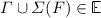
• 2. If $L \, \mathtt {owner}\; \wedge \; L.\mathtt {flag}= \bot$, $\mathtt {Inv}(\mathtt {H}(\varGamma ,L,G)) \, \wedge \, \mathtt {Osafe}(\varGamma ,L,G)$ with:

  

  and $\varLambda .\mathtt {sent}\subseteq \mathtt {supp}(L) \, \wedge \; \overline{\mathtt {rmv}} \not \in \varLambda .\mathtt {sync}.\mathtt {channels}$. If its flag is down, an owner L can reconfigure into an hypercell G, provided G and the cells in L’s scope remaining after the transition (those such that $\mathtt {incl}(\varSigma (G),M)$ have been removed) respect the global invariant $\mathtt {Inv}$, and the roles in the scope of owners in G are either ones already in its scope, or brand new ones. If a cell is an owner, the same constraint as above on sent roles apply, but in addition it cannot be removed by any other cell.

• 3. If $L \,\mathtt {owner}\wedge L.\mathtt {flag}= \top$, $L.\mathtt {owned}\subseteq G.\mathtt {owned}$, , and $\varLambda .\mathtt {sent}\subseteq \mathtt {supp}(L) \, \wedge \; \overline{\mathtt {rmv}} \not \in \varLambda .\mathtt {sync}.\mathtt {channels}$. If its flag is up, an owner can only change into a single owner cell, not losing any owned role, possibly adding some (e.g. to allow the reconfiguration of cells it owns).

• 4. If $L \,\mathtt {free}$, $\mathtt {Inv}(G) \wedge \mathtt {Fsafe}(\varGamma ,L,G)$ where:

  

  and $\varLambda .\mathtt {sent}\subseteq \mathtt {supp}(L)$. A free cell can reconfigure into a hypercell G provided it respects the global invariant $\mathtt {Inv}$, it does not insert new cells in the scope of existing owners, and the roles of cells in the scope of new owners in G are safe. Also, since it is not an owner, new roles created during a transition cannot be immediately sent.

Note that, with the above definition of $\mathtt {Auth}$, in an environment $\varGamma$ where cell L is owned and the flag of its owner M is down, i.e. $\exists M \in \varGamma , \; M \multimap L \wedge M.\mathtt {flag}= \bot$, then L cannot evolve in environment $\varGamma$.

The authorization predicate is quite permissive in the kinds of evolutions owner cells can perform. Notice in particular that owner cells may split or dissolve during execution, allowing e.g. for the transfer of owned cells from one owner to another. Likewise, owned cells can be freed by their owner and become owner cells later on. The dynamicity and concurrency in the class of hypercell models obeying strict encapsulation is much bigger than that allowed in the computational models underlying ownership types (either strictly sequential or actor like).

Predicate $\mathtt {Inv}$ is indeed an invariant for the class of hypercell models equipped with these sorts and authorization functions:

Proposition 2

($\mathtt {Inv}$ is an invariant). For all , if $\mathtt {Inv}(\varGamma )$, $\mathtt {Inv}(G)$ and $\varGamma \vdash G \xrightarrow {\varLambda } G'$, then $\mathtt {Inv}(G')$.

4.2 Selective Encapsulation

We extend the strict encapsulation policy of the previous section with a notion of weak ownership. Briefly, owner scopes of strict encapsulation are now allowed to include weakly owned cells. A cell may belong to only one owner, as previously, but may also belong to several weak owners. A cell can be weakly owned only if it has identified specific provided roles for this purpose ($\mathtt {wprov}$ roles below).

We extend sorts to 6-tuples $\langle k, \mathbf {p}, \mathbf {o}, \mathbf {r}, \mathbf {q}, \mathbf {w} \rangle$ with . We set $\mathfrak {s}.\mathtt {wowned}= \mathbf {w}$ and $\mathfrak {s}.\mathtt {wprov}= \mathbf {q}$. We write

$C.\mathtt {wowned}$ for $C.\mathtt {sort}.\mathtt {wowned}$, and $C.\mathtt {wprov}$ for $C.\mathtt {sort}.\mathtt {wprov}$. $C.\mathtt {wowned}$ are required roles for binding to a weakly owned cell. $C.\mathtt {wprov}$ are provided roles for binding to a weak owner.

We adapt the invariant (1) as follows:

$$\begin{aligned} \begin{aligned} C.\mathtt {prov}= \;&C.\mathtt {fprov}\cup C.\mathtt {wprov}\, \wedge \, C.\mathtt {fprov}\cap C.\mathtt {wprov}= \emptyset \\&\wedge C.\mathtt {req}= C.\mathtt {owned}\cup C.\mathtt {wowned}\cup C.\mathtt {freq}\\&\wedge C.\mathtt {owned}, C.\mathtt {wowned}, C.\mathtt {freq}\,\text {mutually disjoint} \end{aligned} \end{aligned}$$

(5)

For (or ), we write $L\mathrel {\begin{array}{c} \rightharpoonup \end{array}}M$ for $L.\mathtt {wowned}\cap M.\mathtt {wprov}\ne \emptyset$.

Writing now $G.(\mathtt {roles}-\mathtt {wroles})$ for $G.\mathtt {roles}\setminus (G.\mathtt {wowned}\cup G.\mathtt {wprov})$, and

$F \diamond G$ for $F.(\mathtt {roles}-\mathtt {wroles}) \cap G.(\mathtt {roles}-\mathtt {wroles}) = \emptyset$ he global structural invariant is now the conjunction of the following properties:

$$\begin{aligned}&\forall L, M\in G, L\ne M \implies \mathtt {scope}_G(L)\diamond \mathtt {scope}_G(M)\wedge L.\mathtt {owned}\cap M.\mathtt {owned}= \emptyset \end{aligned}$$

(6)

$$\begin{aligned}&\forall L, M\in G, L\multimap M \implies M.\mathtt {owned}= \emptyset \end{aligned}$$

(7)

$$\begin{aligned}&\forall L,M,N \in G, \; L \multimap M \wedge M \smallfrown N \implies L \multimap N \vee L = N \vee M\mathrel {\begin{array}{c} \rightharpoonup \end{array}}N \vee N\mathrel {\begin{array}{c} \rightharpoonup \end{array}}M \end{aligned}$$

(8)

Notice how the invariant (8) changes from the strict encapsulation policy. Cells in an owner scope are now allowed to bind to cells they weakly own, i.e.  the weak ownership relation allows cells to bind roles across group boundaries.

The authorization predicate for this new policy is defined as in the previous section, with just a change in the definition of the $\mathtt {Safe}$ predicate. $\mathtt {Safe}$ is now defined as follows:

Using this policy, we can describe the architecture described in Fig. 1 as a hypercell with cells $C,C_1,C_2,L,L_1,L_2$, where C and L are owners of cells $C_1,C_2$ and $L_1,L_2$, respectively, and where $C_1$ and $C_2$ are weak owners of $L_1$ and $L_2$, respectively.

As it is, the selective encapsulation policy just allows for specifically identified roles to break the encapsulation policy, and for weakly owned cells to act as shared internal means of communication between different owner scopes. It is possible, however, to enforce additional constraints on weak ownership to reflect different aggregation semantics. For instance, one could enforce a lifetime dependency between weak owner and weak owned cell, preventing the removal of a weak owner if its weakly owned cells are still in place, or, one could ensure a cell has a single weak owner. We do not present these examples here, but our two examples in this section should provide a good taste of the possibilities offered.

5 Conclusion

We have presented the Hypercell framework for defining software component models (hypercell models). The basic ontology of any hypercell model agrees with the classical elements of software component models [16, 21], but the combination of dynamicity, sharing and encapsulation an hypercell model can offer is, to the best of our knowledge, unique. The key points to retain are the following: (i) this combination is made possible by the use of contextual transitions, cell sorts and context dependent runtime checks that enforce encapsulation policies; (ii) a proper notion of equivalence between hypercells is obtained thanks to authorizations at the level of individual cells and a notion of bisimulation that decouples the effect of authorizations from the classical bisimulation game.

Our runtime approach to enforcing encapsulation policies seems more permissive, and able to express more forms of policies and aggregations semantics than possible with ownership types, as our examples suggest. However, we have at this time no formal proof of this. Also, how our approach compares with those combining static ownership discipline with dynamic ownership tests, as in the Mezzo permission-based language [1], remains to be seen. It is worth pointing out that in defining encapsulation policies in the Hypercell framework, we do have a choice between imposing static constraints on unconstrained transitions, and imposing dynamic constraints via authorization predicates. In this paper, we have opted in our examples for an approach that made maximal use of authorization, but other options are available that combine both. For expressivity, however, we believe some amount of run-time checking is inescapable.

A crucial question is of course whether our abstract Hypercell framework can be efficiently implemented and supported. An implementation of an abstract machine for object-based hypercells is currently under way, but is clear that enforcing encapsulation constraints via runtime checks is a viable option, as demonstrated by the work on Siaam [15]. This work showed, in the simpler context of the actor model, that the overhead of such checks can largely be mitigated by means of static analyses that can safely remove most unnecessary ones.

References

Balabonski, T., Pottier, F., Protzenko, J.: The design and formalization of Mezzo, a permission-based programming language. ACM Trans. Program. Lang. Syst. 38(4), 14 (2016)
Barbier, F., Henderson-Sellers, B., Le Parc, A., Bruel, J.M.: Formalization of the whole-part relationship in the unified modeling language. IEEE Trans. Softw. Eng. 29(5), 459–470 (2003)
Bass, L., Clements, P., Kazman, R.: Software Architecture in Practice SEI Series in Software Engineering, 3rd edn. Addison-Wesley, Boston (2013)
Bauer, S., et al.: Moving from specifications to contracts in component-based design. In: de Lara, J., Zisman, A. (eds.) FASE 2012. LNCS, vol. 7212, pp. 43–58. Springer, Heidelberg (2012). https://doi.org/10.1007/978-3-642-28872-2_3
Bengtson, J., Johansson, M., Parrow, J., Victor, B.: Psi-calculi: a framework for mobile processes with nominal data and logic. Log. Methods Comput. Sci. 7(1), 1–44 (2011)
Bliudze, S., Sifakis, J.: A notion of glue expressiveness for component-based systems. In: van Breugel, F., Chechik, M. (eds.) CONCUR 2008. LNCS, vol. 5201, pp. 508–522. Springer, Heidelberg (2008). https://doi.org/10.1007/978-3-540-85361-9_39
Bloom, B., Istrail, S., Meyer, A.R.: Bisimulation can’t be traced. J. ACM 42(1), 232–268 (1995)
Bruneton, E., Coupaye, T., Leclercq, M., Quema, V., Stefani, J.B.: The fractal component model and its support in Java. Softw. Pract. Exp. 36(11–12), 1257–1284 (2006)
Bruni, R., Montanari, U., Sammartino, M.: Reconfigurable and software-defined networks of connectors and components. In: Wirsing, M., Hölzl, M., Koch, N., Mayer, P. (eds.) Software Engineering for Collective Autonomic Systems. LNCS, vol. 8998, pp. 73–106. Springer, Cham (2015). https://doi.org/10.1007/978-3-319-16310-9_2
Bugliesi, M., Castagna, G., Crafa, S.: Access control for mobile agents: the calculus of boxed ambients. ACM. Trans. Program. Lang. Syst. 26(1), 57–124 (2004)
Cardelli, L., Gordon, A.: Mobile ambients. Theor. Comput. Sci. 240(1), 177–213 (2000)
Castellani, I.: Process algebras with localities. In: Bergstra, J., Ponse, A., Smolka, S. (eds.) Handbook of Process Algebra, Elsevier (2001)
Cattani, G.L., Sewell, P.: Models for name-passing processes: interleaving and causal. Inf. Comput. 190(2), 136–178 (2004)
Clarke, D., Östlund, J., Sergey, I., Wrigstad, T.: Ownership types: a survey. In: Clarke, D., Noble, J., Wrigstad, T. (eds.) Aliasing in Object-Oriented Programming. Types, Analysis and Verification. LNCS, vol. 7850, pp. 15–58. Springer, Heidelberg (2013). https://doi.org/10.1007/978-3-642-36946-9_3
Claudel, B., Sabah, Q., Stefani, J.B.: Simple isolation for an actor abstract machine. In: Graf, S., Viswanathan, M. (eds.) Formal Techniques for Distributed Objects, Components, and Systems, FORTE 2015. Lecture Notes in Computer Science, vol. 9039. Springer, Cham (2015). https://doi.org/10.1007/978-3-319-19195-9_14
Crnkovic, I., Sentilles, S., Vulgarakis, A., Chaudron, M.R.V.: A classification framework for software component models. IEEE Trans. Softw. Eng. 37(5), 599–615 (2011)
Nicola, R.D., Loreti, M., Pugliese, R., Tiezzi, F.: A formal approach to autonomic systems programming: the SCEL language. ACM Trans. Auton. Adapt. Syst. 9(2), 7 (2014)
Eker, J., et al.: Taming heterogeneity-the Ptolemy approach. Proc. IEEE 91(1), 127–144 (2003)
Ferrari, G.L., Hirsch, D., Lanese, I., Montanari, U., Tuosto, E.: Synchronised hyperedge replacement as a model for service oriented computing. In: de Boer, F.S., Bonsangue, M.M., Graf, S., de Roever, W.-P. (eds.) FMCO 2005. LNCS, vol. 4111, pp. 22–43. Springer, Heidelberg (2006). https://doi.org/10.1007/11804192_2
Fiadeiro, J.L., Lopes, A.: A model for dynamic reconfiguration in service-oriented architectures. Softw. Syst. Model. 12(2), 349–367 (2013)
Garlan, D., Monroe, R.T., Wile, D.: Acme: architectural description of component-based systems. Foundations of Component-Based Systems. Cambridge University Press (2000)
Hennessy, M., Rathke, J., Yoshida, N.: SAFEDPI: a language for controlling mobile code. Acta Inf. 42(4–5), 227–290 (2005)
Jongmans, S.S.T.Q., Arbab, F.: Overview of thirty semantic formalisms for Reo. Sci. Ann. Comput. Sci. 22(1), 201–251 (2012)
Leavens, G., Sitaraman, M. (eds.): Foundations of Component-Based Systems. Cambridge University Press (2000)
Zhiming, L., He, J. (eds.): Mathematical Frameworks for Component Software - Models for Analysis and Synthesis. World Scientic (2006)
Magee, J., Kramer, J.: Dynamic structure in software architectures. In: 4th ACM symposium on Foundations of Software Engineering (FSE-4). ACM (1995)
Merle, P., Stefani, J.B.: A formal specification of the fractal component model in alloy. Research Report RR-6721, INRIA, France (2008)
Milner, R.: The Space and Motion of Communicating Agents. Cambridge University Press, Cambridge (2009)
De Nicola, R., Ferrari, G.L., Pugliese, R.: Klaim: a kernel language for agents interaction and mobility. IEEE Trans. Softw. Eng. 24(5), 315–330 (1998)
Pitts, A.M.: Nominal Sets: Names and Symmetry in Computer Science. Cambridge University Press, Cambridge (2013)
Riely, J., Hennessy, M.: A typed language for distributed mobile processes. In: 25th ACM SIGPLAN-SIGACT Symposium on Principles of Programming Languages (POPL). ACM (1998)
Sanchez, A., Barbosa, L.S., Riesco, D.: Bigraphical modelling of architectural patterns. In: Arbab, F., Ölveczky, P.C. (eds.) FACS 2011. LNCS, vol. 7253, pp. 313–330. Springer, Heidelberg (2012). https://doi.org/10.1007/978-3-642-35743-5_19
Sangiorgi, D., Walker, D.: The \(\pi \)-calculus: A Theory of Mobile Processes. Cambridge University Press, Cambridge (2001)
Schmitt, A., Stefani, J.-B.: The kell calculus: a family of higher-order distributed process calculi. In: Priami, C., Quaglia, P. (eds.) GC 2004. LNCS, vol. 3267, pp. 146–178. Springer, Heidelberg (2005). https://doi.org/10.1007/978-3-540-31794-4_9
Sevegnani, M., Calder, M.: Bigraphs with sharing. Theor. Comput. Sci. 577, 43–73 (2015)
Stefani, J.-B.: Components as location graphs. In: Lanese, I., Madelaine, E. (eds.) FACS 2014. LNCS, vol. 8997, pp. 3–23. Springer, Cham (2015). https://doi.org/10.1007/978-3-319-15317-9_1
Tutu, I., Fiadeiro, J.L.: Service-oriented logic programming. Log. Methods Comput. Sci. 11(3), 1–37 (2015)
van Glabbeek, R.J.: The meaning of negative premises in transition system specifications II. J. Log. Algebraic Program. 60–61, 229–258 (2004). https://www.sciencedirect.com/journal/the-journal-of-logic-and-algebraic-programming/vol/60/suppl/C
Voigt, J.: Access contracts: a dynamic approach to object-oriented access protection. Technical report UCAM-CL-TR-880, University of Cambridge (2016)
Wermelinger, M., Fiadeiro, J.L.: A graph transformation approach to software architecture reconfiguration. Sci. Comput. Program. 44(2), 133–155 (2002)
Author information
Authors and Affiliations
Corresponding authors
Editor information
Editors and Affiliations
Rights and permissions
Copyright information
© 2019 IFIP International Federation for Information Processing
About this paper
Cite this paper
Stefani, JB., Vassor, M. (2019). Encapsulation and Sharing in Dynamic Software Architectures: The Hypercell Framework. In: Pérez, J., Yoshida, N. (eds) Formal Techniques for Distributed Objects, Components, and Systems. FORTE 2019. Lecture Notes in Computer Science(), vol 11535. Springer, Cham. https://doi.org/10.1007/978-3-030-21759-4_14
Download citation
DOI: https://doi.org/10.1007/978-3-030-21759-4_14
Published:
Publisher Name: Springer, Cham
Print ISBN: 978-3-030-21758-7
Online ISBN: 978-3-030-21759-4
eBook Packages: Computer ScienceComputer Science (R0)