Universal Graphs and Good for Games Automata: New Tools for Infinite Duration Games

Abstract

In this paper, we give a self contained presentation of a recent breakthrough in the theory of infinite duration games: the existence of a quasipolynomial time algorithm for solving parity games. We introduce for this purpose two new notions: good for small games automata and universal graphs.

The first object, good for small games automata, induces a generic algorithm for solving games by reduction to safety games. We show that it is in a strong sense equivalent to the second object, universal graphs, which is a combinatorial notion easier to reason with. Our equivalence result is very generic in that it holds for all existential memoryless winning conditions, not only for parity conditions.

This work was supported by the European Research Council (ERC) under the European Union’s Horizon 2020 research and innovation programme (grant agreement No. 670624), and by the DeLTA ANR project (ANR-16-CE40-0007).

1 Introduction

In this abstract, we are interested in the complexity of deciding the winner of finite turn-based perfect-information antagonistic two-player games. So typically, we are interested in parity games, or mean-payoff games, or Rabin games, etc$\ldots$

In particular we revisit the recent advances showing that deciding the winner of parity games can be done in quasipolynomial time. Whether parity games can be solved in polynomial time is the main open question in this research area, and an efficient algorithm would have far-reaching consequences in verification, synthesis, logic, and optimisation. From a complexity-theoretic point of view, this is an intriguing puzzle: the decision problem is in NP and in coNP, implying that it is very unlikely to be NP-complete (otherwise NP = coNP). Yet no polynomial time algorithm has yet been constructed. For decades the best algorithms were exponential or mildly subexponential, most of them of the form $n^{O(d)}$, where $n$ is the number of vertices and $d$ the number of priorities (we refer to Section 2 for the role of these parameters).

Recently, Calude, Jain, Khoussainov, Li, and Stephan [CJK+17] constructed a quasipolynomial time algorithm for solving parity games, of complexity $n^{O(\log d)}$. Two subsequent algorithms with similar complexity were constructed by Jurdziński and Lazić [JL17], and by Lehtinen [Leh18].

Our aim in this paper is to understand these results through the prism of good for small games automata, which are used to construct generic reductions to solving safety games. A good for small games automaton can be understood as an approximation of the original winning condition which is correct for small games. The size of good for small games automata being critical in the complexity of these algorithms, we aim at understanding this parameter better.

A concrete instanciation of good for small games automata is the notion of separating automata, which was introduced by Bojańczyk and Czerwiński [BC18] to reformulate the first quasipolynomial time algorithm of [CJK+17]. Later Czerwiński, Daviaud, Fijalkow, Jurdziński, Lazić, and Parys [CDF+19] showed that the other two quasipolynomial time algorithms also can be understood as the construction of separating automata, and proved a quasipolynomial lower bound on the size of separating automata.

In this paper, we establish in particular Theorem 9 which states an equivalence between the size of good for small games automata, non-deterministic of separating automata, of deterministic separating automata and of universal graphs. This statement is generic in the sense that it holds for any winning condition which is memoryless for the existential player, hence in particular for parity conditions. At a technical level, the key notion that we introduce to show this equivalence is the combinatorial concept of universal graphs.

Our second contribution, Theorem 10, holds for the parity condition only, and is a new equivalence between universal trees and universal graphs. In particular we use a technique of saturation of graphs which simplifies greatly the arguments. The two theorems together give an alternative simpler proof of the result in [CDF+19].

Let us mention that the equivalence results have been very recently used to construct algorithms for mean-payoff games, leading to improvements over the best known algorithm [FGO18].

Structure of the paper In Section 2 we introduce the classical notions of games, automata, and good for games automata. In Section 3, we introduce the notion of good for small games automata, and show that in the context of memoryless for the existential player winning conditions these automata can be characterised in different ways, using in particular universal graphs (Theorem 9). In Section 4, we study more precisely the case of parity conditions.

2 Games and automata

We describe in this subsection classical material: arenas, games, strategies, automata and good for games automata. Section 2.1 introduces games, Section 2.2 the concept of memoryless strategy, and Section 2.3 the class of automata we use. Finally, Section 2.4 explains how automata can be used for solving games, and in particular defines the notion of automata that are good for games.

2.1 Games

We will consider several forms of graphs, which are all directed labelled graph with a root vertex. Let us fix the terminology now. Given a set $X$, an $X$-graph $H=(V,E,\text {root}_{H})$ has a set of vertices $V$, a set of $X$-labelled edges $E\subseteq V\times X\times V$, and a root vertex . We write if there exists a path from vertex $x$ to vertex $y$ labelled by the word $u\in X^*$. We write if there exists an infinite path starting in vertex $x$ labelled by the word $u\in X^\omega$. The graph is trimmed if all vertices are reachable from the root and have out-degree at least one. Note that as soon as a graph contains some infinite path starting from the root, it can be made trimmed by removing the bad vertices. A morphism of $X$-graphs from $G$ to $H$ is a map $\alpha$ from vertices of $G$ to vertices of $H$, that sends the root of $G$ to the root of $H$, and sends each edge of $G$ to an edge of $H$, i.e., for all $a\in X$, implies . A weak morphism of $X$-graphs is like a morphism but we lift the property that the root of $G$ is sent to the root of $H$ and instead require that if then .

Definition 1

Let  be a set (of colors). A $C$-arena $A$ is a $C$-graph in which vertices are split into $V=V_\mathrm{E}\uplus V_\mathrm{A}$. The vertices are called positions. The positions in $V_\mathrm{E}$ are the positions owned by the existential player, and the ones in $V_\mathrm{A}$ are owned by the universal player. The root is the initial position. The edges are called moves. Infinite paths starting in the initial position are called plays. Finite paths starting in the initial position are called partial plays. The dual of an arena is obtained by swapping $V_\mathrm{A}$ and $V_\mathrm{E}$, i.e., exchanging the ownernship of the positions.

A $\mathbb W$-game  consists of a $C$-arena $A$ together with a set called the winning condition.

For simplicity, we assume in this paper the following epsilon property¹: there is a special color  such that for all words $u,v\in C^\omega$, if $u$ and $v$ are equal after removing all the $\varepsilon$-letters, then $u\in \mathbb W$ if and only if $v\in \mathbb W$.

The dual of a game is obtained by dualising the arena, and complementing the winning condition.

If one compares with usual games – for instance checkers – then the arena represents the set of possible board configurations of the game (typically, the configuration of the board plus a bit telling whose turn to play it is). The configuration is an existential position if it is the first player’s turn to play, otherwise it is a universal position. There is an edge from u to v if it is a valid move for the player to go from configuration u to configuration v. The interest of having colors and winning conditions may not appear clearly in this context, but the intent would be, for example, to tell who is the winner if the play is infinite.

Informally, the game is played as follows by two players: the existential player and the universal player². At the beginning, a token is placed at the initial position of the game. Then the game proceeds in rounds. At each round, if the token is on an existential position then it is the existential player’s turn to play, otherwise it is the universal player’s turn. This player chooses an outgoing move from the position, and the token is pushed along this move. This interaction continues forever, inducing a play (defined as an infinite path in the arena) labelled by an infinite sequence of colors. If this infinite sequence belongs to the winning condition $\mathbb W$, then the existential player wins the play, otherwise, the universal player wins the play. It may happen that a player has to play but there is no move available from the current position: in this case the player immediately loses.

Classical winning conditions Before describing more precisely the semantics of games, let us recall what are the classical winning conditions considered in this context.

Definition 2

We define the following classical winning conditions:  

safety condition :

The safety condition is  over the unique color 0. Expressed differently, all plays are winning. Note that the color 0 fulfills the requirement of the epsilon property.

Muller condition :

Given a finite set of colors $C$, a Muller condition is a Boolean combination of winning conditions of the form “the color c appears infinitely often”. In general, no color fulfills the requirement of the epsilon property, but it is always possible to add an extra fresh color $\varepsilon$. The resulting condition satisfies the epsilon property.

Rabin condition :

Given a number p, we define the Rabin condition by $u\in \mathtt {Rabin}_p$ if there exists some $i \in 1, \ldots , p$ such that when projected on this component, 2 appears infinitely often in $u$, and 3 finitely often. Note that the constant vector $\mathbf 1$ fulfills the epsilon property. The Rabin condition is a special case of Muller conditions.

parity condition :

Given a interval of integers $C=[i,j]$ (called priorities), a word $u=c_1c_2c_3\cdots \in C^\omega$ belongs to  if the largest color appearing infinitely often in $u$ is even.

Büchi condition :

The Büchi condition  is a parity condition over the restricted interval [1, 2] of priorities. A word belongs to $\mathtt {Buchi}$ if it contains infinitely many occurrences of 2.

coBüchi condition :

The coBüchi condition  is a parity condition over the restricted interval [0, 1] of priorities. A word belongs to $\mathtt {coBuchi}$ if it it has only finitely many occurrences of 1’s.

mean-payoff condition :

Given a finite set , a word $u=c_1c_2c_3\cdots \in C^\omega$ belongs to  if

$$\begin{aligned} \liminf _{n\rightarrow \infty }\frac{c_1+c_2+\cdots +c_{n}}{n} \geqslant 0\ . \end{aligned}$$

There are many variants of this definition (such as replacing $\liminf$ with $\limsup$), that all turn out to be equivalent on finite arenas.

 

Strategies We describe now formally what it means to win a game. Let us take the point of view of the existential player. A strategy for the existential player is an object that describes how to play in every situation of the game that could be reached. It is a winning strategy if whenever these choices are respected during a play, the existential player wins this play. There are several ways one can define the notion of a strategy. Here we choose to describe a strategy as the set of partial plays that may be produced when it is used.

Definition 3

A strategy s for the existential player $s_\mathrm{E}$ is a set of partial plays of the game that has the following properties:

• $s_\mathrm{E}$ is prefix-closed and non-empty,

• for all partial plays $\pi \in s_\mathrm{E}$ ending in some $v\in V_\mathrm{E}$, there exists exactly one partial play of length $|\pi |+1$ in $s_\mathrm{E}$ that prolongs $\pi$,

• for all partial plays $\pi \in s_\mathrm{E}$ ending in some $v\in V_\mathrm{A}$, then all partial plays that prolong $\pi$ of length $|\pi |+1$ belong to $s_\mathrm{E}$.

A play is compatible with the strategy $s_\mathrm{E}$ if all its finite prefixes belong to $s$. A play is winning if it belongs to the winning condition $\mathbb W$. A game is won by the existential player if there exists a strategy for the existential player such that all plays compatible with it are won by the existential player. Such a strategy is called a winning strategy.

Symmetrically, a (winning) strategy for the universal player is a (winning) strategy for the existential player in the dual game. A game is won by the universal player if there exists a strategy for the universal player such that all infinite plays compatible with it are won by the universal player.

The idea behind this definition is that at any moment in the game, when following a strategy, a sequence of moves has already been played, yielding a partial play in the arena. The above definition guarantees that: 1. if a partial play belongs to the strategy, it is indeed reachable by a succession of moves that stay in the strategy, 2. if, while following the strategy, a partial play ends in a vertex owned by the existential player, there exists exactly one move that can be followed by the strategy at that moment, and 3. if, while following the strategy, a partial play ends in a vertex owned by the universal player, the strategy is able to face all possible choices of the opponent.

Remark 1

It is not possible that in a strategy defined in this way one reaches an existential position that would have no successor: indeed, 2. would not hold.

Remark 2

There are different ways to define a strategy in the literature. One is as a strategy tree: indeed one can see $s_\mathrm{E}$ as a set of nodes equipped with prefix ordering as the ancestor relation. Another way is to define a strategy as a partial map from paths to moves. All these definitions are equivalent. The literature also considers randomized strategies (in which the next move is chosen following a probability distribution): this is essential when the games are concurrent or with partial information, but not in the situation we consider in this paper.

Lemma 1

(at most one player wins). It is not possible that both the existential player and the universal player win the same game.

Of course, keeping the intuition of games in mind, one would expect also that one of the player wins. However, this is not necessarily the case. A game is called determined if either the existential or the universal player wins the game. The fact that a game is determined is referred to as its determinacy. A winning condition $\mathbb W$ is determined if all $\mathbb W$-games are determined. It happens that not all games are determined.

Theorem 1

There exist winning conditions that are not determined (and it requires the axiom of choice to prove it).

However, there are some situations in which games are determined. This is the case of finite duration games, of safety games, and more generally:

Theorem 2

(Martin’s theorem of Borel determinacy [Mar75]). Games with Borel winning conditions are determined.

Defining the notion of Borel sets is beyond the scope of this paper. It suffices to know that this notion is sufficiently powerful for capturing a lot of natural winning conditions, and in particular all winning conditions in this paper are Borel; and thus determined.

2.2 Memory of strategies

A key insight in understanding a winning condition is to study the amount of memory required by winning strategies. To define the notion of memoryless strategies, we use an equivalent point of view on strategies, using strategy graphs.

Definition 4

Given a $C$-arena $A$, an existential player strategy graph $S_\mathrm{E},\gamma$ in $A$ is a trimmed $C$-graph $S_\mathrm{E}$ together with a graph morphism $\gamma$ from $S_\mathrm{E}$ to $A$ such that for all vertices $x$ in $S_\mathrm{E}$,

• if $\gamma (x)$ is an existential position, then there exists exactly one edge of the form $(x,c,y)$ in $S_\mathrm{E}$,

• if $\gamma (x)$ is a universal position, then $\beta$ induces a surjection between the edges originating from x in $S_\mathrm{E}$ and the moves originating from $\beta (x)$, i.e., for all moves of the form $(\beta (x),c,v)$, there exists an edge of the form $(x,c,y)$ in $S_\mathrm{E}$ such that $\beta (y)=v$.

The existential player strategy graph $S_\mathrm{E},\gamma$ is memoryless if $\gamma$ is injective. In general the memory of the strategy is the maximal cardinality of $\gamma ^{-1}(v)$ for v ranging over all positions in the arena. For  a $\mathbb W$-game with $\mathbb W\subseteq C^\omega$, an existential player strategy graph $S_\mathrm{E}$ is winning if the labels of all its paths issued from the root belong to $\mathbb W$.

The (winning) universal player strategy graphs are defined as the (winning) existential player strategy graphs in the dual game.

The winning condition $\mathbb W$ is memoryless for the existential player if, whenever the existential player wins in a $\mathbb W$-game, there is a memoryless winning existential player strategy graph. It is memoryless for the existential player over finite arenas if this holds for finite $\mathbb W$-games only. The dual notion is the one of memoryless for the universal player winning condition.

Of course, as far as existence is concerned the two notions of strategy coincide:

Lemma 2

There exists a winning existential player strategy graph if and only if there exists a winning strategy for the existential player.

Proof

A strategy for the existential player $s_\mathrm{E}$ can be seen as a $C$-graph (in fact a tree) $S_\mathrm{E}$ of vertices $s_\mathrm{E}$, of root $\varepsilon$, and with edges of the form $(\pi ,a,\pi a)$ for all $\pi a\in s_\mathrm{E}$. If the strategy $s_\mathrm{E}$ is winning, then the strategy graph $S_\mathrm{E}$ is also winning. Conversely, given an existential player strategy graph $S_\mathrm{E}$, the set $s_\mathrm{E}$ of its paths starting from the root is itself a strategy for the existential player. Again, the winning property is preserved.□

We list a number of important results stating that some winning conditions do not require memory.

Theorem 3

([EJ91]). The parity condition is memoryless for the existential player and for the universal player.

Theorem 4

([EM79, GKK88]). The mean-payoff condition is memoryless for the existential player over finite arenas as well as for the universal player.

Theorem 5

([GH82]). The Rabin condition is memoryless for the existential player, but not in general for the universal player.

Theorem 6

([McN93]). Muller conditions are finite-memory for both players.

Theorem 7

([CFH14]). Topologically closed conditions for which the residuals are totally ordered by inclusion are memoryless for the existential player.

2.3 Automata

Definition 5

(automata over infinite words). Let . A (non-deterministic) $\mathbb W$-automaton $\mathcal {A}$ over the alphabet $A$ is a $(C\times A)$-graph. The convention is to call states its vertices, and transitions its edges. The root vertex is called the initial state. The set $\mathbb W$ is called the accepting condition (whereas it is the winning condition for games). The automaton is obtained from $\mathcal {A}$ by setting the state $p$ to be initial.

A run of the automaton $\mathcal {A}$ over $u\in A^\omega$ is an infinite path in $\mathcal {A}$ that starts in the initial state and projects on its $A$-component to $u$. A run is accepting if it projects on its $C$-component to a word $v\in \mathbb W$. The language accepted by $\mathcal {A}$ is the set  of infinite words $u\in A^\omega$ such that there exists an accepting run of $\mathcal {A}$ on u.

An automaton is deterministic (resp. complete) if for all states p and all letters $a\in A$, there exists at most one (resp. at least one) transition of the form (p, (a, c), q). If the winning condition is parity, this is a parity automaton. If the winning condition is safety, this is a safety automaton, and we do not mention the $C$-component since there is only one color. I.e., the transitions form a subset of $Q\times A\times Q$, and the notion coincides with the one of a $A$-graph. For this reason, we may refer to the language $\mathcal {L}(H)$ accepted by an $A$-graph $H$: this is the set of labelling words of infinite paths starting in the root vertex of $H$.

Note that here we use non-deterministic automata for simplicity. However, the notions developed in this paper can be adapted to alternating automata.

The notion of $\omega$-regularity. It is not the purpose of this paper to describe the rich theory of automata over infinite words. It suffices to say that a robust concept of $\omega$-regular language emerges. These are the languages that are equivalently defined by means of Büchi automata, parity automata, Rabin automata, Muller automata, deterministic parity automata, deterministic Rabin automata, deterministic Muller automata, as well as many other formalisms (regular expressions, monadic second-order logic, $\omega$-semigroup, alternating automata, $\ldots$). However, safety automata and deterministic Büchi automata define a subclass of $\omega$-regular languages.

Note that the mean-payoff condition does not fall in this category, and automata defined with this condition do not recognize $\omega$-regular languages in general.

2.4 Automata for solving games

There is a long tradition of using automata for solving games. The general principle is to use automata as reductions, i.e. starting from a $\mathbb V$-game  and a $\mathbb W$-automaton  that accepts the language $\mathbb V$, we construct a $\mathbb W$-game $\mathcal {G}\times \mathcal {A}$ called the product game that combines the two, and which is expected to have the same winner: this means that to solve the $\mathbb V$-game $\mathcal {G}$, it is enough to solve the $\mathbb W$-game $\mathcal {G}\times \mathcal {A}$. We shall see below that, unfortunately, this expected property does not always hold (Remark 4). The automata that guarantee the correction of the construction are called good for games, originally introduced by Henzinger and Piterman [HP06].

We begin our description by making precise the notion of product game. Informally, the new game requires the players to play like in the original game, and after each step, the existential player is required to provide a transition in the automaton that carries the same label.

Definition 6

Let  be an arena over colors , with positions  and moves . Let also  be a $\mathbb W$-automaton over the alphabet $C$ with states and transitions . We construct the product arena as follows:

• The set of positions in the product game is $(P\uplus M)\times Q$.

• The initial position is , in which is the initial position of $\mathcal {G}$, and is the initial state of $\mathcal {A}$.

• The positions of the form $(x,p)\in P\times Q$ are called game positions and are owned by the owner of $x$ in $\mathcal {G}$. There is a move, called a game move, of the form $((x,p),\varepsilon ,((x,c,y),p))$ for all moves $(x,c,y)\in M$.

• The positions of the form $((x,c,y),p)\in M\times Q$ are called automaton positions and are owned by the existential player. There is a move, called an automaton move, of the form $(((x,c,y),p),d,(y,q))$ for all transitions of the form $(p,(c,d),q)$ in $\mathcal {A}$.

Note that every game move $((x,p),\varepsilon ,((x,c,y),p))$ of $\mathcal {G}\times \mathcal {A}$ can be transformed into a move $(x,c,y)$ of $\mathcal {G}$, called its game projection. Similarly every automaton move $(((x,c,y),p),d,(y,q))$ can be turned into a transition $(p,(c,d),q)$ of the automaton $\mathcal {A}$ called its automaton projection. Hence, every play $\pi$ of the product game can be projected into the pair of a play $\pi ^\prime$ in $\mathcal {G}$ of label $u$ (called the game projection), and an infinite run $\rho$ of the automaton over $u$ (called the automaton projection). The product game is the game over the product arena, using the winning condition of the automaton.

Lemma 3

(folklore³). Let  be a $\mathbb V$-game, and  be a $\mathbb W$-automaton that accepts a language , then if the existential player wins $\mathcal {G}\times Q_{\mathcal A}$, she wins $\mathcal {G}$.

Proof

Assume that the existential player wins the game $\mathcal {G}\times \mathcal {A}$ using a strategy $s_\mathrm{E}$. This strategy can be turned into a strategy for the existential player $s^\prime _\mathrm{E}$ in $\mathcal {G}$ by performing a game projection. It is routine to check that this is a valid strategy.

Let us show that this strategy $s^\prime _\mathrm{E}$ is $\mathbb V$-winning, and hence conclude that the existential player wins the game $\mathcal {G}$. Indeed, let $\pi ^\prime$ be a play compatible with $s^\prime _\mathrm{E}$, say labelled by $u$. This play $\pi ^\prime$ has been obtained by game projection of a play $\pi$ compatible with $s_\mathrm{E}$ in $\mathcal {G}\times \mathcal {A}$. The automaton projection $\rho$ of $\pi$ is a run of $\mathcal {A}$ over $u$, and is accepting since $s_\mathrm{E}$ is a winning strategy. Hence, $u$ is accepted by $\mathcal {A}$ and as a consequence belongs to $\mathbb V$. We have proved that $s_\mathrm{E}$ is winning.□

Corollary 1

Let  be a $\mathbb V$-game, and be a deterministic $\mathbb W$-automaton that accepts the language $\mathbb V$, then the games $\mathcal {G}$ and $\mathcal {G}\times \mathcal {A}$ have the same winner.

Proof

We assume without loss of generality that $\mathcal {A}$ is deterministic and complete (note that this may require to slightly change the accepting condition, for instance in the case of safety). The results then follows from the application of Lemma 3 to the game $\mathcal {G}$ and its dual.□

The consequence of the above lemma is that when we know how to solve $\mathbb W$-games, and we have a deterministic $\mathbb W$-automaton $\mathcal {A}$ for a language $\mathbb V$, then we can decide the winner of $\mathbb V$-games by performing the product of the game with the automaton, and deciding the winner of the resulting game. Good for games automata are automata that need not be deterministic, but for which this kind of arguments still works.

Definition 7

(good for games automata [HP06]). Let  be a language, and  be a $\mathbb W$-automaton. Then $\mathcal {A}$ is good for $\mathbb V$-games if for all $\mathbb V$-games $\mathcal {G}$, $\mathcal {G}$ and $\mathcal {G}\times \mathcal {A}$ have the same winner.

Note that Lemma 1 says that deterministic automata are good for games automata.

Remark 3

It may seem strange, a priori, not to require in the definition that $\mathcal {L}(\mathcal {A})=\mathbb V$. In fact, it holds anyway: if an automaton is good for $\mathbb V$-games, then it accepts the language $\mathbb V$. Indeed, let us assume that there exists a word $u\in \mathcal {L}(\mathcal {A})\setminus \mathbb V$, then one can construct a game that has exactly one play, labelled $u$. This game is won by the universal player since $u\not \in \mathbb V$, but the existential player wins $\mathcal {G}\times \mathcal {A}$. A contradiction. The same argument works if there is a word in $\mathbb V\setminus \mathcal {L}(\mathcal {A})$.

Examples of good for games automata can be found in [BKS17], together with a structural analysis of the extent to which they are non-deterministic.

Remark 4

We construct an automaton which is not good for games. The alphabet is $\{a,b\}$. The automaton is a Büchi automaton: it has an initial state from which goes two $\epsilon$-transitions: the first transition guesses that the word contains infinitely many a’s, and the second transition guesses that the word contains infinitely many b’s. Note that any infinite word contains either infinitely many a’s or infinitely many b’s, so the language recognised by this automaton is the set of all words. However, this automaton requires a choice to be made at the very first step about which of the two alternatives hold. This makes it not good for games: indeed, consider a game  where the universal player picks any infinite word, letter by letter, and the winning condition is $\mathbb V$. It has only one position owned by the universal player. The existential player wins $\mathcal {G}$ because all plays are winning. However, the existential player loses $\mathcal {G}\times \mathcal {A}$, because in this game she has to declare at the first step whether there will be infinitely many a’s or infinitely many b’s, which the universal player can later contradict.

Let us conclude this part with Lemma 4, stating the possibility to compose good for games automata. We need before hand to defined the composition of automata.

Given $A\times B$-graph $\mathcal {A}$, and $B\times C$-graph $\mathcal {B}$, the composed graph  has as states the product of the sets of states, as initial state the ordered pair of the initial states, and there is a transition $((p,q),(a,c),(p^\prime ,q^\prime ))$ if there is a transition $(p,(a,b),p^\prime )$ in $\mathcal {A}$ and a transition $(q,(b,c),q^\prime )$. If $\mathcal {A}$ is in fact an automaton that uses the accepting condition , and $\mathcal {B}$ an automaton that uses the accepting condition , then the composed automaton  uses has as underlying graph the composed graphs, and as accepting condition $\mathbb W$.

Lemma 4

(composition of good for games automata). Let  be a good for games $\mathbb W$-automaton for the language , and  be good for games $\mathbb V$-automaton for the language $L$, then the composed automaton $\mathcal {A}\circ \mathcal {B}$ is a good for games $\mathbb W$-automaton for the language $L$.

3 Efficiently solving games

From now on, graphs, games and automata are assumed to be finite.

We now present more recent material. We put forward the notion of good for n-games automata (good for small games) as a common explanation for the several recent algorithms for solving parity games ‘efficiently’. After describing this notion in Section 3.1, we shall give more insight about it in the context of winning conditions that are memoryless for the existential player in Section 3.2

Much more can be said for parity games and good for small games safety automata: this will be the subject of Section 4.

3.1 Good for small games automata

We introduce the concept of (strongly) good for n-games automata (good for small games). The use of these automata is the same as for good for games automata, except that they are cannot be composed with any game, but only with small ones. In other words, a good for $(\mathbb W,n)$-game automaton yields a reduction for solving $\mathbb W$-games with at most $n$ positions (Lemma 6). We shall see in Section 3.2 that as soon as the underlying winning condition is memoryless for the existential player, there are several characterisations for the smallest strongly good for n-games automata. It is good to keep in mind the definition of good for games automata (Definition 7) when reading the following one.

Definition 8

Let  be a language, and  be a $\mathbb W$-automaton. Then $\mathcal {A}$ is good for $(\mathbb V,n)$-games if for all $\mathbb V$-games $\mathcal {G}$ with at most $n$ positions, $\mathcal {G}$ and $\mathcal {G}\times \mathcal {A}$ have the same winner (we also write good for small games when there is no need for $\mathbb V$ and $n$ to be explicit).

It is strongly good for $(\mathbb V,n)$-games if it is good for $(\mathbb V,n)$-games and the language accepted by $\mathcal {A}$ is contained in $\mathbb V$.

Example 1

(automata that are good for small games). We have naturally the following chain of implications:

The first implication is from Remark 3, and the second is by definition. Thus the first examples of automata that are strongly good for small games are the automata that are good for games.

Example 2

We consider the case of the coBüchi condition: recall that the set of colors is $\{0,1\}$ and the winning plays are the ones such that there ultimately contain only 0’s. It can be shown that if the existential player wins in a coBüchi game with has at most $n$ positions, then she also wins for the winning condition $L=(0^*(\varepsilon +1))^{n} 0^\omega$, i.e., the words in which there is at most $n$ occurrences of 1 (indeed, a winning memoryless strategy for the condition $\mathtt {coBuchi}$ cannot contain a 1 in a cycle, and hence cannot contain more than $n$ occurrences of 1 in the same play; thus the same strategy is also winning in the same game with the new winning condition $L$). As a consequence, a deterministic safety automaton that accepts the language $L\subseteq \mathtt {coBuchi}$ (the minimal one has $n+1$ states) is good for $(\mathtt {coBuchi},n)$-games.

Mimicking Lemma 4 which states the closure under composition of good for games automata, we obtain the following variant for good for small games automata:

Lemma 5

(composition of good for small games automata). Let  be a good for $n$-games $\mathbb V$-automaton for the language $L$ with $k$ states, and be a good for $kn$-games $\mathbb W$-automaton for the language , then the composed automaton $\mathcal {A}\circ \mathcal {B}$ is a good for n-games $\mathbb W$-automaton for the language $L$.

We also directly get an algorithm from such reductions.

Lemma 6

Assume that there exists an algorithm for solving $\mathbb W$-games of size $\lim$ in time $f(m)$. Let be a $\mathbb V$-game with at most $n$ positions and be a good for $(\mathbb V,n)$-games $\mathbb W$-automaton of size $k$, there exists an algorithm for solving $\mathcal {G}$ of complexity $f(kn)$.

Proof

Construct the game $\mathcal {G}\times \mathcal {A}$, and solve it.□

The third quasipolynomial time algorithm for solving parity games due to Lehtinen [Leh18] can be phrased using good for small games automata (note that it is not originally described in this form).

Theorem 8

([Leh18, BL19]).Given positive integers $n,d$, there exists a parity automaton with $n^{(\log d+ O(1))}$ states and $1 + \lfloor \log n\rfloor$ priorities which is strongly good for $n$-games.

Theorem 8 combined with Lemma 6 yields a quasipolynomial time algorithm for solving parity games. Indeed, consider a parity game with $n$ positions and d priorities. Let be the good for $n$-games automaton constructed by Theorem 8. The game $\mathcal {G}\times \mathcal {A}$ is a parity game equivalent to $\mathcal {G}$, which has $\lim = n^{(\log d+ O(1))}$ states and $d^\prime = 1 + \lfloor \log n\rfloor$ priorities. Solving this parity game with a simple algorithm (of complexity $O(m^{d^\prime })$) yields an algorithm of quasipolynomial complexity:

$$ O(m^{d^\prime }) = O( n^{(\log d+ O(1)) d^\prime } ) = n^{O(\log (d) \log (n))}. $$

3.2 The case of memoryless winning conditions

In this section we fix a winning condition $\mathbb W$ which is memoryless for the existential player, and we establish several results characterising the smallest strongly good for small games automata in this case.

Our prime application is the case of parity conditions, that will be studied specifically in Section 4, but this part also applies to conditions such as mean-payoff or Rabin.

The goal is to establish the following theorem (the necessary definitions are introduced during the proof).

Theorem 9

Let  be a winning condition which is memoryless for the existential player, then the following quantities coincide for all positive integers $n$:

• 1. the least number of states of a strongly $(\mathbb W, n)$-separating deterministic safety automaton,

• 2. the least number of states of a strongly good for $(\mathbb W, n)$-games safety automaton,

• 3. the least number of states of a strongly $(\mathbb W, n)$-separating safety automaton,

• 4. the least number of vertices of a $(\mathbb W, n)$-universal graph.

The idea of separating automata⁴ was introduced by Bojańczyk and Czerwiński [BC18] to reformulate the first quasipolynomial time algorithm [CJK+17]. Czerwiński, Daviaud, Fijalkow, Jurdziński, Lazić, and Parys [CDF+19] showed that the other two quasipolynomial time algorithms [JL17, Leh18] also can be understood as the construction of separating automata.

The proof of Theorem 9 spans over Sections 3.2 and 3.3. It it a consequence of Lemmas 7, 8, 11, and 12. We begin our proof of Theorem 9 by describing the notion of strongly separating automata.

Definition 9

An automaton  is strongly $(\mathbb W, n)$-separating if

$$\begin{aligned} \mathbb W|_n\subseteq \mathcal {L}(\mathcal {A})\subseteq \mathbb W\ , \end{aligned}$$

in which is the union of all the languages accepted by safety automata with $n$ states that accept sublanguages of $\mathbb W$.⁵

Lemma 7

In the statement of Theorem 9, (1) $\Longrightarrow$ (2) $\Longrightarrow$ (3).

Proof

Assume (1), i.e., there exists a strongly $(\mathbb W,n)$-separating deterministic safety automaton , then $\mathcal {L}(\mathcal {A})\subseteq \mathbb W$. Let  be a $\mathbb W$-game with at most $n$ positions. By Lemma 3, if the existential player wins $\mathcal {G}\times \mathcal {A}$, she wins the game $\mathcal {G}$. Conversely, assume that the existential player wins $\mathcal {G}$, then, by assumption she has a winning memoryless strategy graph $S_\mathrm{E},\gamma :S_\mathrm{E}\rightarrow \mathcal {G}$, i.e., $\mathcal {L}(S_\mathrm{E})\subseteq \mathbb W$ and $\gamma$ is injective. By injectivity of $\gamma$, $S_\mathrm{E}$ has at most $n$ vertices and hence $\mathcal {L}(S_\mathrm{E})\subseteq \mathbb W|_n\subseteq \mathcal {L}(\mathcal {A})$. As a consequence, for every (partial) play $\pi$ compatible with $S_\mathrm{E}$, there exists a (partial) run of $\mathcal {A}$ over the labels of $\pi$ (call this property ). We construct a new strategy for the existential player in $\mathcal {G}\times \mathcal {A}$ as follows: When the token is in a game position, the existential player plays as in $S_\mathrm{E}$; When the token is in an automaton position, the existential player plays the only available move (indeed, the move exists by property , and is unique by the determinism assumption). Since this is a safety game, the new strategy is winning. Hence the existential player wins $\mathcal {G}\times \mathcal {A}$, proving that $\mathcal {A}$ is good for $(\mathbb W, n)$-games. Item 2 is established.

Assume now (2), i.e., that  is some strongly good for $(\mathbb W, n)$-games automaton. Then by definition $\mathcal {L}(\mathcal {A})\subseteq \mathbb W$. Now consider some word $u$ in $\mathbb W|_n$. By definition, there exists some safety automaton  with at most $n$ states such that $u\in \mathcal {L}(\mathcal {B})\subseteq \mathbb W$. This automaton can be seen as a $\mathbb W$-game  in which all positions are owned by the universal player. Since $\mathcal {L}(\mathcal {B})\subseteq \mathbb W$, the existential player wins the game $\mathcal {G}$. Since furthermore $\mathcal {A}$ is good for $(\mathbb W, n)$-games, the existential player has a winning strategy $S_\mathrm{E}$ in $\mathcal {G}\times \mathcal {A}$. Assume now that the universal player is playing the letters of $u$ in the game $\mathcal {G}\times \mathcal {A}$, then the winning strategy $S_\mathrm{E}$ constructs an accepting run of $\mathcal {A}$ on $u$. Thus $u\in \mathcal {L}(\mathcal {A})$, and Item 3 is established.□

We continue our proof of Theorem 9 by introducing the notion of $(\mathbb W, n)$-universal graph.

Definition 10

Given a winning condition  and a positive integer $n$, a $C$-graph $U$ is $(\mathbb W, n)$-universal⁶ if

• $\mathcal {L}(U)\subseteq \mathbb W$, and

• for all $C$-graphs $H$ such that $\mathcal {L}(U)\subseteq \mathbb W$ and with at most $n$ vertices, there is a weak graph morphism from $H$ to $U$.

We are now ready to prove one more implication of Theorem 9.

Lemma 8

In the statement of Theorem 9, (4) $\Longrightarrow$ (1)

Proof

Assume that there is a $(\mathbb W,n)$-universal graph $U$. We show that $U$ seen as an safety automaton is strongly good for $(\mathbb W, n)$-games. One part is straightforward: $\mathcal {L}(U)\subseteq \mathbb W$ is by assumption. For the other part, consider a $\mathbb W$-game  with at most $n$ positions. Assume that the existential player wins $\mathcal {G}$, this means that there exists a winning memoryless strategy for the existential player $S_\mathrm{E},\gamma :S_\mathrm{E}\rightarrow \mathcal {G}$ in $\mathcal {G}$. We then construct a strategy for the existential player $S^\prime _\mathrm{E}$ that maintains the property that the only game positions in $\mathcal {G}\times U$ that are met in $S^\prime _\mathrm{E}$ are of the form $(x,\gamma (x))$. This is done as follows: when a game position is encountered, the existential player plays like the strategy $S_\mathrm{E}$, and when an automaton position is encountered, the existential player plays in order to follow $\gamma$. This is possible since $\gamma$ is a weak graph morphism.□

3.3 Maximal graphs

In order to continue our proof of Theorem 9, more insight is needed: we have to understand what are the $\mathbb W$-maximal graphs. This is what we do now.

Definition 11

A $C$-graph $H$ is $\mathbb W$-maximal if $\mathcal {L}(H)\subseteq \mathbb W$ and if it is not possible to add a single edge to it without breaking this property, i.e., without producing an infinite path from the root vertex that does not belong to $\mathbb W$.

Lemma 9

For a winning condition  which is memoryless for the existential player, and $H$ a $\mathbb W$-maximal graph, then the $\varepsilon$-edges in $H$ form a transitive and total relation.

Proof

Transitivity arises from the epsilon property of winning conditions (Definition 1): Consider three vertices $x$, $y$ and $z$ such that $\alpha =(x,\varepsilon ,y)$ and $\beta =(y,\varepsilon ,z)$ are edges of $H$. Let us add a new edge $\delta =(x,\varepsilon ,y)$ yielding a new graph $H^\prime$. Let us consider now any infinite path $\pi$ in $H^\prime$ starting in the root (this path may contain finitely of infinitely many occurrences of $\delta$, but not almost only $\delta$’s since $x\ne y$). Let $\pi ^\prime$ be obtained from $\pi$ by replacing each occurrence of $\delta$ by the sequence $\alpha \beta$. The resulting path $\pi ^\prime$ belongs $H$, and thus its labelling belongs to $\mathbb W$. But since the labelings of $\pi$ and $\pi ^\prime$ agree after removing all the occurrences of $\varepsilon$, the epsilon property guarantees that the labelling of $\pi$ belongs to $\mathbb W$. Since this holds for all choices of $\pi$, we obtain $\mathcal {L}(H^\prime )\subseteq \mathbb W$. Hence, by maximality, $\delta \in H$, which means that the $\varepsilon$-edges form a transitive relation.

Let us prove the totality. Let $x$ and $y$ be distinct vertices of $H$. We have to show that either  or . We can turn $H$ into a game  as follows:

• all the vertices of $H$ become positions that are owned by the universal player and we add a new position $z$ owned by the existential player;

• all the edges of $H$ that end in $x$ or $y$ become moves of $\mathcal {G}$ that now end in $z$,

• all the other edges of $H$ become moves of $\mathcal {G}$ without change,

• and there are two new moves in $\mathcal {G}$, $(z,\varepsilon ,x)$ and $(z,\varepsilon ,y)$.

We claim first that the game $\mathcal {G}$ is won by the existential player. Let us construct a strategy $s_\mathrm{E}$ in $\mathcal {G}$ as follows. The only moment the existential player has a choice to make is when the play reaches the position $z$. This has to happen after a move of the form $(t,a,z)$. This move originates either from an edge of the form $(t,a,x)$, or from an edge of the form $(t,a,y)$. In the first case the strategy $s_\mathrm{E}$ chooses the move $(z,\varepsilon ,x)$, and in the second case the move $(z,\varepsilon ,y)$. Let us consider a play $\pi$ compatible with $s_\mathrm{E}$, and let $\pi ^\prime$ be obtained from $\pi$ by replacing each occurrence of $(t,a,z)(z,\varepsilon ,x)$ with $(t,a,x)$ and each occurrence of $(t,a,z)(z,\varepsilon ,y)$ with $(t,a,y)$. The resulting $\pi ^\prime$ is a path in $H$ and hence its labeling belongs to $\mathbb W$. Since the labelings of $\pi$ and $\pi ^\prime$ are equivalent up to $\varepsilon$-letters, by the epsilon property, the labeling of $\pi$ also belongs to $\mathbb W$. Hence the strategy $s_\mathrm{E}$ witnesses the victory of the existential player in $\mathcal {G}$. The claim is proved.

By assumption on $\mathbb W$, this means that there exists a winning memoryless strategy for the existential player $S_\mathrm{E}$ in $\mathcal {G}$. In this strategy, either the existential player always chooses $(z,\varepsilon ,x)$, or she always chooses $(z,\varepsilon ,y)$. Up to symmetry, we can assume the first case. Let now $H^\prime$ be the graph $H$ to which a new edge $\delta =(y,\varepsilon ,x)$ has been added. We aim that $\mathcal {L}(H^\prime )\subseteq \mathbb W$. Let $\pi$ be an infinite path in $H^\prime$ starting from the root vertex. In this path, each occurrences of $\delta$ are preceded by an edge of the form $(t,a,y)$. Thus, let $\pi ^\prime$ be obtained from $\pi$ by replacing each occurrence of a sequence of the form $(t,a,y)\delta$ by $(t,a,y)$. The resulting path is a play compatible with $S_\mathrm{E}$. Hence the labeling of $\pi ^\prime$ belongs to $\mathbb W$, and as a consequence, by the epsilon property, this is also the case for $\pi$. Since this holds for all choices of $\pi$, we obtain that $\mathcal {L}(H^\prime )\subseteq \mathbb W$. Hence, by $\mathbb W$-maximality assumption, $(y,\varepsilon ,x)$ is an edge of $H$.

Overall, the $\varepsilon$-edges form a total transitive relation.□

Let  be the least relation closed under reflexivity and that extends the $\varepsilon$-edge relation.

Lemma 10

For a winning condition  which is memoryless for the existential player, and $H$ a $\mathbb W$-maximal graph, then the following properties hold:

• The relation $\leqslant _{\varepsilon }$ is a total preorder.

• implies , for all vertices $x^\prime ,x,y,y^\prime$ and colors $a$.

• For all vertices $p,q$, if and only $q\leqslant _{\varepsilon }p$.

• for all vertices $p,q$ and colors $a$, if and only if .

Proof

The first part is obvious from Lemma 9. For the second part, it is sufficient to prove that implies and that implies . Both cases are are similar to the proof of transitivity in Lemma 9⁷. The two next items are almost the same. The difficult direction is to assume the language inclusion, and deduce the existence of an edge (left to right). Let us assume for an instant that $H$ would be a finite word automaton, with all its states accepting. Then it is an obvious induction to show that if (as languages of finite words), it is safe to add an $\varepsilon$-transitions from $q$ to $p$ without changing the language. The two above items are then obtained by limit passing (this is possible because the safety condition is topologically closed).□

We are now ready to provide the missing proofs for Theorem 9: from (3) to (4), and from (3) to (1). Both implications arise from Lemma 9.

Lemma 11

In the statement of Theorem 9, (3) $\Longrightarrow$ (4).

Proof

Let us start from a strongly $(\mathbb W,n)$-separating safety automaton . Without loss of generality, we can assume it is $\mathbb W$-maximal. We claim that it is $(\mathbb W,n)$-universal.

Let us define first for all languages $K\subseteq C^\omega$, its closure

(in case of an empty intersection, we assume $C^\omega$). This is a closure operator: $K\subseteq K'$ implies $\overline{K}\subseteq \overline{K'}$, $K\subseteq \overline{K}$, and $\overline{\overline{K}}=\overline{K}$. Futhermore, $a\overline{K}\subseteq \overline{aK}$, for all letters $a\in C$. Let now $H$ be a trimmed graph with at most $n$ vertices such that $\mathcal {L}(H)\subseteq \mathbb W$. We have $\mathcal {L}(H)\subseteq \mathbb W|_n$ by definition of $\mathbb W|_n$.

We claim that for each vertex $x$ of $H$, there is a state $\alpha (x)$ of $\mathcal {A}$ such that

Indeed, note first that, since $H$ is trimmed, there exists some word $u$ such that . Hence, using the fact that $\mathcal {A}$ is strongly $(\mathbb W,n)$-separating, we get that for all , $uv\in \mathcal {L}(H)\subseteq \mathbb W|_n\subseteq \mathcal {L}(\mathcal {A})$. Let $\beta (v)$ be the state assumed after reading $u$ by a run of $\mathcal {A}$ accepting $uv$. It is such that . Since $\mathcal {A}$ is finite and its states are totally ordered under inclusion of residuals (Lemma 10), this means that there exists a state $\alpha (x)$ (namely the maximum over all the $\beta (w)$ for ) such that .

Let us show that $\alpha$ is a weak graph morphism⁸ from $H$ to $\mathcal {A}$. Consider some edge $(x,a,y)$ of $H$. We have . Hence

which implies by Lemma 10 that . Let now  be some edge. By hypothesis, we have

Thus . We obtain  by Lemma 10. Hence, $\alpha$ is a weak graph morphism.

Since this holds for all choices of $H$, we have proved that $\mathcal {A}$ is a $(\mathbb W,n)$-universal graph.□

Lemma 12

In the statement of Theorem 9, (3) $\Longrightarrow$ (1).

Proof

Let us start from a strongly $(\mathbb W,n)$-separating safety automaton . Without loss of generality, we can assume it is maximal. Thus Lemma 10 holds.

We now construct a deterministic safety automaton .

• the states of $\mathcal {D}$ are the same as the states of $\mathcal {A}$,

• the initial state of $\mathcal {D}$ is the initial state of $\mathcal {A}$,

• given a state $p\in \Delta _{\mathcal {D}}$ and a letter $a$, a transition of the form $(p,a,q)$ exists if and only if there is some transition of the form $(p,a,r)$ in $\mathcal {A}$, and $q$ is chosen to be the least state $r$ with this property.

We have to show that this deterministic safety automaton is strongly $(\mathbb W,n)$-separating. Note first that by definition $\mathcal {D}$ is obtained from $\mathcal {A}$ by removing transitions. Hence $\mathcal {L}(\mathcal {D})\subseteq \mathcal {L}(\mathcal {A})\subseteq \mathbb W$. Consider now some $u\in \mathbb W|_n$. By assumption, $u\in \mathcal {L}(\mathcal {A})$. Let $\rho = (p_0,u_1,p_1)(p_1,u_2,p_2)\cdots$ be the corresponding accepting run of $\mathcal {A}$. We construct by induction a (the) run of $\mathcal {D}$ $(q_0,u_1,q_1)(q_1,u_2,q_2)\cdots$ in such a way that $q_i\leqslant _{\varepsilon }p_i$. For the initial state, $p_0=q_0$. Assume the run up to $q_i\leqslant _{\varepsilon }p_i$ has been constructed. By Lemma 10, $(q_i,u_{i+1},p_{i+1})$ is a transition of $\mathcal {A}$. Hence the least $r$ such that $(q_i,u_{i+1},r)$ is a transition of $\mathcal {A}$ does exist, and is $\leqslant _{\varepsilon }p_{i+1}$. Let us call it $q_{i+1}$; we indeed have that $(q_i,u_{i+1},q_{i+1})$ is a transition of $\mathcal {D}$. Hence, $u$ is accepted by $\mathcal {D}$. Thus $\mathbb W|_n\subseteq \mathcal {L}(\mathcal {D})$.

Overall $\mathcal {D}$ is a strongly $(\mathbb W,n)$-separating deterministic safety automaton that has at most as many states as $\mathcal {A}$.□

4 The case of parity conditions

We have seen above some general results on the notion of universal graphs, separating automata, and automata that are good for small games. In particular, we have seen Theorem 9 showing the equivalence of these objects for memoryless for the existential player winning conditions.

We are paying now a closer attention to the particular case of the parity condition. The technical developments that follow give an alternative proof of the equivalence results proved in [CDF+19] between strongly separating automata and universal trees.

4.1 Parity and cycles

We begin with a first classical lemma, which reduces the questions of satisfying a parity condition to checking the parity of cycles.

In a directed graph labelled by priorities, an even cycle is a cycle (all cycles are directed) such that the maximal priority occurring in it is even. Otherwise, it is an odd cycle. As usual, an elementary cycle is a cycle that does not meet twice the same vertex.

Lemma 13

For a $[i,j]$-graph $H$ that has all its vertices reachable from the root, the following properties are equivalent:

• $\mathcal {L}(H)\subseteq \mathtt {Parity}_{[i,j]}$,

• having all its cycles even,

• having all its elementary cycles even.

Proof

Clearly, since all vertices are reachable, $\mathcal {L}(H)\subseteq \mathbb W$ implies that all the cycles are even. Also, if all cycles are even, then all elementary cycles also are. Finally assume that all the elementary cycles are even. Then we can consider $H$ as a game, in which every positions is owned by the universal player. Assume that some infinite path from the root would not satisfy $\mathtt {Parity}_{[i,j]}$, then this path would be a winning strategy for the universal player in this game. Since $\mathtt {Parity}_{[i,j]}$ is a winning condition memoryless for the universal player, this means that the universal player has a winning memoryless strategy. But this winning memoryless strategy is nothing but a lasso, and thus contains an elementary cycle of maximal odd priority.□

4.2 The shape and size of universal graphs for parity games

We continue with a fixed d, and we consider parity conditions using priorities in [0, 2d]. More precisely, we relate the size of universal graphs for the parity condition with priorities [0, 2d] to universal d-trees as defined now:

Definition 12

A $d$-tree $t$ is a balanced, unranked, ordered tree of height $d$ (the root does not count: all branches contain exactly $d+1$ nodes). The order between nodes of same level is denoted . Given a leaf $x$, and $i=0\ldots i$, we denote the ancestor at depth $i$ of $x$ (0 is the root, $d$ is $x$).

The $d$-tree $t$ is $n$-universal if for all $d$-trees $s$ with at most $n$ nodes, there is a $d$-tree embedding of $s$ into $t$, in which a $d$-tree embedding is an injective mapping from nodes of $s$ to nodes of $t$ that preserves the height of nodes, the ancestor relation, and the order of nodes. Said differently, $s$ is obtained from $t$ by pruning some subtrees (while keeping the structure of a $d$-tree).

Definition 13

Given a $d$-tree $t$, is a $[0,2d]$-graph with the following characteristics:

• the vertices are the leaves of t,

• for $0\leqslant i\leqslant d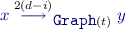$, if ,

• for $0<i\leqslant d$, if .

Lemma 14

For all $d$-trees $t$, $\mathcal {L}(\mathtt {Graph}(t))\subseteq \mathtt {Parity}_{[0,2d]}$.

Proof

Using Lemma 13, it is sufficient to prove that all cycle in $\mathtt {Graph}(t)$ are even. Thus, let us consider a cycle $\rho$. Assume that the highest priority occurring in $\alpha$ is $2(d-i)+1$. Note then that for all edges $\alpha =(x,k,y)$ occurring in $\rho$:

• since $k\leqslant i+1$,

• if $k=2(d-i)+1$, .

As a consequence, the first and last vertex of $\alpha$ cannot have the same ancestor at level $i$, and thus are different.□

Below, we develop sufficient results for establishing:

Theorem 10

([CF18]). For all positive integers $d,n$, the two following quantities are equal:

• the smallest number of leaves of an $n$-universal $d$-tree, and

• the smallest number of vertices of a $(\mathtt {Parity}_{[0,2d]},n)$-universal graph.

Proof

We shall see below (Definition 14) a construction $\mathtt {Tree}$ that maps all $\mathtt {Parity}_{[0,2d]}$-maximal graphs $G$ to a $d$-tree $\mathtt {Tree}(G)$ of smaller or same size. Corollary 4 establishes that this construction is in some sense the converse of $\mathtt {Tree}$ (in fact they form an adjunction). and that this correspondence preserves the notions of universality. This proves the above result: Given a $n$-universal $d$-tree $t$, then, by Corollary 4, $\mathtt {Graph}(t)$ is a $(\mathtt {Parity}_{[0,2d]},n)$-universal graph that has as many vertices as leaves of graphs. Conversely, consider a $(\mathtt {Parity}_{[0,2d]},n)$-universal graph $G$. One can add to it edges until it becomes a $\mathtt {Parity}_{[0,2d]}$-maximal graph $G^\prime$ with as many vertices. Then, by Corollary 4, $\mathtt {Tree}(G^\prime )$ is an $n$-universal $d$-tree that has as much or less leaves than vertices of $G^\prime$.□

Example 3

The complete $d$-tree $t$ of degree $n$ (that has $n^{d}$ leaves) is $n$-universal. The $[0,2d]$-graph $\mathtt {Graph}(t)$ obtained in this way is used in the small progress measure algorithm [Jur00].

However, there exists $n$-universal $d$-trees that are much smaller than in the above example. The next theorem provides an upper and a lower bound.

Theorem 11

([Fij18, CDF+19]). Given positive integers $n,d$,

• there exists an $n$-universal $d$-tree with

  $$ n \cdot \left( {\begin{array}{c}\lceil \log (n) \rceil + d - 1\\ \lceil \log (n) \rceil \end{array}}\right) $$

  leaves.

• all $n$-universal $d$-trees have at least

  $$ \left( {\begin{array}{c}\lfloor \log (n) \rfloor + d - 1\\ \lfloor \log (n) \rfloor \end{array}}\right) $$

  leaves.

Corollary 2

The complexity of solving $\mathtt {Parity}_{[0,d]}$-games with at most $n$-vertices is

$$ O\left( m n \log (n) \log (d) \cdot \left( {\begin{array}{c}\lceil \log (n) \rceil + d/2 - 1\\ \lceil \log (n) \rceil \end{array}}\right) \right) . $$

and no algorithm based on good for small safety games can be faster than quasipolynomial time.

Maximal universal graphs for the parity condition

We shall now analyse in detail the shape of $\mathtt {Parity}_{[0,2d]}$-maximal graphs. This analysis culminates with the precise description of such graphs in Lemma 19, that essentially establishes a bijection with graphs of the form $\mathtt {Graph}(t)$ (Corollary 4).

Let us note that, since the parity condition is memoryless for the existential player, using Lemma 10, and the fact that the parity condition is unchanged by modifying finite prefixes, we can always assume that the root vertex is the minimal one for the $\leqslant _{\varepsilon }$ ordering. Thus, from now, we do not have to pay attention to the root, in particular in weak graph morphisms. Thus, from now, we just mention the term morphism for weak graph morphisms.

Let us recall preference ordering $\sqsubseteq$ between the non-negative integers is defined as follows:

$$\begin{aligned} \cdots \sqsubset 2d+1\sqsubset 2d-1\sqsubset \cdots \sqsubset 3\sqsubset 1\sqsubset 0\sqsubset 2\sqsubset \cdots \sqsubset 2d-2\sqsubset 2d\sqsubset \cdots \end{aligned}$$

Fact 1

Let $k\sqsubseteq \ell$ and $u,v$ sequences of priorities. If the maximal priority occurring in $ukv$ is even, then the maximal priority occurring in $u\ell v$ is also even.

Lemma 15

Let $G$ be a $\mathtt {Parity}_{[0,2d]}$-maximal graph and $k\sqsubseteq \ell$ be priorities in $[0,2d]$. For all vertices $x,y$ of $G$, implies .

Proof

Let us add $(x,\ell ,y)$ to $G$. Let $u(x,\ell ,y)v$ be some elementary cycle of the new graph involving the new edge $(x,\ell ,y)$. By Lemma 13, $u(x,k,y)v$ is an even cycle in the original graph. Hence, by Fact 1, $u(x,\ell ,y)v$ is also an even cycle. Thus, by Lemma 13, $G$ with the newly added edge also satisfies $\mathcal {L}(G)\subseteq \mathtt {Parity}_{[0,2d]}$. Using the maximality assumption for $G$, we obtain that $(x,\ell ,y)$ was already present in $G$.□

Lemma 16

Let $G$ be a $\mathtt {Parity}_{[0,2d]}$-maximal graph. For all vertices $x,y,z$ of $G$, if and , then .

Proof

Let us add $(x,\max (k,\ell ),z)$ to $G$. Let $u(x,\max (k,\ell ),z)v$ be an elementary cycle in the new graph. By Lemma 13, $u(x,k,y)(y,\ell ,z)v$, being a cycle of $G$, has to be even. Since, furthermore, the maximal priority that occurs in $u(x,k,y)(y,\ell ,z)v$ is the same as the maximal one in $u(x,\max (k,\ell ),z)v$, the cycle $u(x,\max (k,\ell ),z)v$ is also even. Using the maximality assumption of $G$, we obtain that $(x,\max (k,\ell ),z)$ was already present in $G$.□

Lemma 17

Let $G$ be a $\mathtt {Parity}_{[0,2d]}$-maximal graph, and $x,y$ be vertices, then , and .

Proof

For , it is sufficient to notice that adding the edge $(x,0,x)$, if it was not present, simply creates one new elementary cycle to $G$, namely $(x,0,x)$. Since it is an even cycle, by Lemma 13, the new graph also satisfies $\mathcal {L}(G)\subseteq \mathtt {Parity}_{[0,2d]}$. Hence, by maximality assumption, the edge was already present in $G$ before.

Consider the graph $G$ with an extra edge $(x,2d,y)$ added. Consider now an elementary cycle that contains $(x,2d,y)$, i.e., of the form $u(x,2d,y)v$. Its maximal priority is $2d$, and thus even. Hence by Lemma 13 and maximality assumption, the edge was already present in $G$.□

Lemma 18

Let $G$ be a $\mathtt {Parity}_{[0,2d]}$-maximal graph and $k=0,2,\ldots ,2d-2$. For all vertices $x,y$, holds if and only if does not hold.

Proof

Assume first that and both holds. Then is an odd cycle contradicting Lemma 13.

Conversely, assume that adding the edge  would break the property $\mathcal {L}(G)\subseteq \mathtt {Parity}_{[0,2d]}$. This means that there is an elementary cycle of the form $u(x,k+1,y)v$ which is odd. Let $\ell$ be the maximal priority in $vu$. If $\ell \geqslant k+1$, then  $\ell$ is odd, and thus $\ell \sqsubseteq k$, and we obtain by Lemma 15. Otherwise, $\ell \leqslant k$, and again $\ell \sqsubseteq k$. Once more holds by Lemma 15.□

Lemma 19

A $[0,2d]$-graph $G$ is a $\mathtt {Parity}_{[0,2d]}$-maximal graph if and only if all the following properties hold:

• 1. is a total preorder for all $k=0,2,\ldots ,2d$,

• 2. for all ,

• 3. is the total equivalence relation,

• 4. for all $k=0,2,\ldots ,2d-2$.⁹

Proof

First direction. Assume first that $G$ is a $\mathtt {Parity}_{[0,2d]}$-maximal graph.

(1) Let $k=0,2,\ldots ,2d$; is transitive by Lemma 16. Furthermore, by Lemma 17, for all vertices $x$, and thus by Lemma 15, since $0\sqsubseteq k$, . Hence is also reflexive and hence a preorder. Consider now another vertex $y$. By Lemma 18, either  or . But by Lemma 15, implies . Hence either  or . Thus  is a total preorder.

(2) For $k=0,2,\ldots ,2d-2$, since $k\sqsubseteq k+2$, by Lemma 15, .

(3) is the maximal relation by Lemma 15.

(4) For $k=0,2,\ldots ,2d-2$ and $x,y$, we know that holds if and only if does not. This shows .

Second direction. Assume now that $G$ satisfies the conditions (1)-(4). Let us first show that $\mathcal {L}(G)\subseteq \mathtt {Parity}_{[0,2d]}$. For the sake of contradiction, consider an elementary cycle that would be odd. It can be written as $u(x,k,y)v$ with a maximal odd priority $k$. Note first that for all $\ell \leqslant k$: indeed, by (2), this is true if $\ell$ is even, and by (1) and (4), for all $j$ odd. Also  is the strict version of the preorder . Hence, the path $u(x,k,y)v$ has to strictly advance with respect to the preorder : it cannot be a cycle.

Assume now that an edge $(x,k,y)$ is not present in $G$. If $k$ is even, since $(x,k,y)$ is not present, by (4) this means that $(y,k+1,x)$ is present. Hence, adding the edge $(x,k,y)$ would create the odd cycle $(x,k,y)(y,k+1,x)$. If $k$ is odd, since $(x,k,y)$ is not present, by (4) this means that $(y,k-1,x)$ is present. Hence, adding the edge $(x,k,y)$ would create the odd cycle $(x,k,y)(y,k-1,x)$. Hence $G$ is $\mathtt {Parity}_{[0,2d]}$-maximal.□

Corollary 3

Given a morphism $\alpha$ from a $\mathtt {Parity}_{[0,2d]}$-maximal graph $H$ to a $\mathtt {Parity}_{[0,2d]}$-maximal graph $G$, then if and only if , for all vertices $x,y$ of $H$ and integers $k$ in $[0,2d]$. Furthermore, if $\alpha$ is surjective, then every map $\beta$ from $G$ to $H$, such that $\alpha \circ \beta$ is the identity on $G$ is an injective morphism.

Proof

First part. From left to right, this is the definition of a morphism. The other direction is by (4) of Lemma 19: if  and $k$ is odd, then does not hold by (4), thus does not hold by morphism, thus holds by (4) again. The case of $k$ even is similar (using $k+1$ this time).

For the second part, since $\alpha \circ \beta$ is the identity, $\beta$ has to be injective. It is a morphism by the first part.□

The next definition, allowing to go from graphs to trees is shown meaningful by Lemma 19:

Definition 14

Let $G$ be a $\mathtt {Parity}_{[0,2d]}$-maximal graph. The $d$-tree is constructed as follows:

• the nodes of level $i=0,\ldots ,d$ are the pairs $(i,C)$ for $C$ ranging over the equivalence classes of ,

• a node $(i,C)$ is an ancestor of $(j,D)$ if $i\leqslant j$ and $D\subseteq C$,

• if  for all $x\in C$ and $x^\prime \in C^\prime$.

We shall see that $\mathtt {Graph}$ and $\mathtt {Tree}$ are almost the inverse one of the other. This is already transparent in the following lemma, which is just a reformulation of the definitions.

Lemma 20

Let $q$ be the quotient map from vertices of $G$ to leaves of $\mathtt {Tree}(G)$ that maps each vertex to its -equivalence class. It has the following property for all vertices $x,y$ of $G$:

The identity maps the vertices of $\mathtt {Graph}(t)$ to the leaves of $t$, and has the property that for all vertices $x,y$:

Corollary 4

¹⁰ For all $\mathtt {Parity}_{[0,2d]}$-maximal graphs $G,H$, all $d$-trees $t$, and all positive integers $n$,

• $\mathtt {Graph}(\mathtt {Tree}(G))$ is a quotient and an induced subgraph of $G$,

• $\mathtt {Tree}(\mathtt {Graph}(t))$ is isomorphic to $t$,

• there is a morphism from $H$ to $\mathtt {Graph}(t)$ if and only if there is a tree embedding from $\mathtt {Tree}(H)$ to $t$,

• $\mathtt {Tree}(G)$ is $n$-universal if and only if $G$ is $(\mathtt {Parity}_{[0,2d]},n)$-universal,

• $\mathtt {Graph}(t)$ is $(\mathtt {Parity}_{[0,2d]},n)$-universal if and only if $t$ is $n$-universal.

Proof

Let $q$ be the quotient from Lemma 20. It can be seen as a surjective map from vertices of $\mathtt {Graph}(\mathtt {Tree}(G))$ to $G$. By Lemma 20 it is a morphism. By Corollary 3, $\mathtt {Graph}(\mathtt {Tree}(G))$ is also an induced subgraph of $G$.

The leaves of $\mathtt {Tree}(\mathtt {Graph}(t))$ are the singletons consisting of leaves of $t$. Hence, there is a bijective map from leaves of $\mathtt {Tree}(\mathtt {Graph}(t))$ to leaves of $t$ that sends$\{\ell \}$ to $\ell$. By Lemma 20, this is a morphism, and by Corollary 3 an isomorphism.

For the third item, assume first that there is a morphism from $H$ to $\mathtt {Graph}(t)$. By the first point, there is an injective morphism from $\mathtt {Graph}(\mathtt {Tree}(H))$ to $H$. By composition, we obtain a morphism from $\mathtt {Graph}(\mathtt {Tree}(H))$ to $\mathtt {Graph}(t)$. By Lemma 20, it is also a tree embedding from $\mathtt {Tree}(H)$ to $t$. Conversely, assume that there exists an embedding from $\mathtt {Tree}(H)$ to $t$. It can be raised by Lemma 20 to a morphism from $\mathtt {Graph}(\mathtt {Tree}(H))$ to $\mathtt {Graph}(t)$. By the first point, there is a morphism from $H$ to $\mathtt {Graph}(\mathtt {Tree}(H))$. By composition, we get a morphism from $H$ to $\mathtt {Graph}(t)$.

The two last items are obvious from the one just before.□