Steps and Traces

Abstract

In the theory of coalgebras, trace semantics can be defined in various distinct ways, including through algebraic logics, the Kleisli category of a monad or its Eilenberg-Moore category. This paper elaborates two new unifying ideas: (1) coalgebraic trace semantics is naturally presented in terms of corecursive algebras, and (2) all three approaches arise as instances of the same abstract setting. Our perspective puts the different approaches under a common roof, and allows to derive conditions under which some of them coincide.

J. Rot—The research leading to these results has received funding from the European Research Council under the European Union’s Seventh Framework Programme (FP7/2007-2013)/ERC grant agreement nr. 320571.

1 Introduction

Traces are used in the semantics of state-based systems as a way of recording the consecutive behaviour of a state in terms of sequences of observable (input and/or output) actions. Trace semantics leads to, for instance, the notion of trace equivalence, which expresses that two states cannot be distinguished by only looking at their iterated in/output behaviour.

For many years already, trace semantics is a central topic of interest in the coalgebra community — and not only there, of course. One of the key features of the area of coalgebra is that states and their coalgebras can be considered in different universes, formalised as categories. The break-through insight is that trace semantics for a system in universe A can often be obtained by switching to a different universe B. More explicitly, where the (ordinary) behaviour of the system can be described via a final coalgebra in universe A, the trace behaviour arises by finality in the different universe B. Typically, the alternative universe B is a category of algebraic logics, the Kleisli category, or the category of Eilenberg-Moore algebras, of a monad on universe A.

This paper elaborates two new unifying ideas.

• 1. We observe that the trace map from the state space of a coalgebra to a carrier of traces is in all three situations the unique ‘coalgebra-to-algebra’ map to a corecursive algebra [6] of traces. This differs from earlier work which tries to describe traces as final coalgebras. For us it is quite natural to view languages as algebras, certainly when they consist of finite words/traces.

• 2. Next, these corecursive algebras, used as spaces of traces, all arise via a uniform construction, in a setting given by an adjunction together with a special natural transformation that we call a ‘step’. We heavily rely on a basic result saying that in this situation, the (lifting of the) right adjoint preserves corecursive algebras, sending them from one universe to another. This is a known result [5], but its fundamental role in trace semantics has not be recognized before. For an arbitrary coalgebra there is then a unique map to the transferred corecursive algebra; this is the trace map that we are after.

The main contribution of this paper is the unifying step-based approach to coalgebraic trace semantics: it is shown that three existing flavours of trace semantics — logical, Eilenberg-Moore, Kleisli — are all instances of our approach. Moreover, comparison results are given relating two of these forms of trace semantics, namely logic-to-Eilenberg-Moore and logic-to-Kleisli. The other combinations involve subtleties which we do not fully grasp yet. Due to space limitations, we don’t cover the whole field of coalgebraic trace semantics: we focus only on finite trace semantics, and also exclude at this stage the ‘iteration’ based approaches, e.g., in [8, 22, 25].

Outline. The paper is organised as follows. It starts in Sect. 1 with the abstract step-and-adjunction setting, and the relevant definitions and results for corecursive algebras. In the next three sections, it is explained how this setting gives rise to trace semantics, by presenting the above-mentioned three approaches to coalgebraic trace semantics in terms of steps and adjunctions: Eilenberg-Moore (Sect. 3), logical (Sect. 4) and Kleisli (Sect. 5). In each case, the relevant corecursive algebra is described. These sections are illustrated with several examples. The next section establishes a connection between the Eilenberg-Moore and the logical approach, and a connection between the Kleisli and logical approach (Sect. 6). In Sect. 7 we briefly show that our construction of corecursive algebras strengthens to a construction of completely iterative algebras. Finally, in Sect. 8 we provide some directions for future work.

Notation.

In the context of an adjunction $F \dashv G$, we shall use overline notation $\overline{(-)}$ for adjoint transposition. The unit and counit of an adjunction are, as usual, written as $\eta$ and $\varepsilon$.

For an endofunctor H, we write $\mathrm {Alg}(H)$ for its algebra category and $\mathrm {CoAlg}(H)$ for its coalgebra category. For a monad $(T,\eta ,\mu )$ on $\mathbf {C}$, we write $\mathcal {E}{}\mathcal {M}(T)$ for the Eilenberg-Moore category and $\mathcal {K}{}\ell (T)$ for the Kleisli category.

We recall that any functor $S :\mathbf {Sets} \rightarrow \mathbf {Sets}$ has a unique strength $\mathrm {st}$. We write $\mathrm {st}:S(X^A) \rightarrow S(X)^A$ for $\mathrm {st}(t)(a) = S(\mathrm {ev}_a)(t)$, where $\mathrm {ev}_a = \lambda f. f(a) :X^A \rightarrow X$.

2 Coalgebraic Semantics from a Step

This section is about the construction of corecursive algebras and their use for semantics. The notion of corecursive algebra, studied in [6, 9] as the dual of Taylor’s notion of recursive coalgebra [10], is defined as follows.

Definition 1

Let H be an endofunctor on a category $\mathbf {C}$.

• 1. A coalgebra-to-algebra morphism from a coalgebra $c:X \rightarrow H(X)$ to an algebra $a:H(A)\rightarrow A$ is a map $f:X \rightarrow A$ such that the diagram

  

  commutes. Equivalently: such a morphism is a fixpoint for the endofunction on the homset $\mathbf {C} (X,A)$ sending f to the composite

  

• 2. An algebra $a :H(A) \rightarrow A$ is corecursive when for every coalgebra $c :H \rightarrow H(X)$ there is a unique coalgebra-to-algebra morphism $(X,c) \rightarrow (A,a)$.

Here is some intuition.

• As explained in [14], the specification of a coalgebra-to-algebra morphism f is a “divide-and-conquer” algorithm. It says: to operate on an argument, first decompose it via the coalgebra c, then operate on each component via H(f), then combine the results via the algebra a.

• For each final H-coalgebra , the inverse $\zeta ^{-1} :H(A) \rightarrow A$ is a corecursive algebra. For most functors of interest, this final coalgebra gives semantics up to bisimilarity, which is finer than trace equivalence. So trace semantics requires a different corecursive algebra.

In all our examples, we use the same procedure for obtaining a corecursive algebra, which we shall now explain. Our basic setting consists of an adjunction, two endofunctors, and a natural transformation:

(1)

The natural transformation $\rho :HG \Rightarrow GL$ will be called a step. Here H is the behaviour functor: we study H-coalgebras and give semantics for them in a corecursive H-algebra. This arrangement is well-known in the area of coalgebraic modal logic [3, 7, 20, 24, 27], but we shall see that its application is wider.

A step can be formulated in several equivalent ways [18, 23].

Theorem 2

In the situation (1), there are bijective correspondences between natural transformations $\rho _1 :HG \Rightarrow GL$, $\rho _2 :FH \Rightarrow LF$, $\rho _3 :FHG \Rightarrow L$ and $\rho _4 :H \Rightarrow GLF$.

Moreover, if H and L happen to be monads, then $\rho _1$ is an $\mathcal {E}{}\mathcal {M}$-law (map $HG \Rightarrow GL$ compatible with the monad structures) iff $\rho _2$ is a $\mathcal {K}{}\ell$-law (map $FH \Rightarrow LF$ compatible with the monad structures) iff $\rho _4$ is a monad map; and two further equivalent characterisations are respectively a lifting of G or an extension of F:

Proof

We only mention the bijective correspondences: $\rho _1$ and $\rho _3$ correspond by adjoint transposition, and similarly for $\rho _2$ and $\rho _4$. Further, $\rho _2$ and $\rho _3$ are obtained from each other by:

$\square$

It is common to refer to $\rho _1$ and $\rho _2$ as mates; the other two maps are their adjoint transposes. In diagrams we omit the subscript i in $\rho _i$ and let the type determine which version of $\rho$ is meant.

Further, in the remainder of this paper we drop the usual subscript of components of natural transformations.

Definition 3

In the setting (1), the step natural transformation $\rho$ gives rise to both:

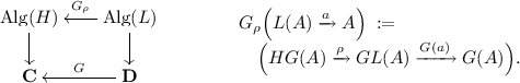
• a lifting $G_\rho$ of the right adjoint G, called the step-induced algebra lifting:

  

• dually, a lifting $F^{\rho }$ of the left adjoint F, called the step-induced coalgebra lifting:

  

Our approach relies on the following basic result.

Proposition 4

([5]). For each corecursive L-algebra $a :L(A) \rightarrow A$, the transferred H-algebra $G_{\rho } (A,a) :HG(A) \rightarrow G(A)$ is also corecursive. Explicitly, for any H-coalgebra (X, c), the unique coalgebra-to-algebra map $(X,c) \rightarrow G_{\rho }(A,a)$ is the adjoint transpose of the unique coalgebra-to-algebra map $F^{\rho }(X,c) \rightarrow (A,a)$. $\square$

Thus, by analogy with the familiar statement that “right adjoints preserves limits”, we have “step-induced algebra liftings of right adjoints preserve corecursiveness”. Now we give the complete construction for semantics of a coalgebra.

Theorem 5

Suppose that L has a final coalgebra . Then for every H-coalgebra (X, c) there is a unique coalgebra-to-algebra map $c^\dagger$ as on the left below:

The map $c^\dagger$ on the left can alternatively be characterized via its adjoint transpose $\overline{c^{\dagger }}$ on the right, which is the unique coalgebra-to-algebra morphism. The latter can also be seen as the unique map to the final coalgebra . $\square$

Note that Theorem 5 generalises final coalgebra semantics: taking in (1) $F = G = \mathrm {Id}_{\mathbf {C}}$ and $H = L$, the map $c^\dagger$ in the above theorem is the unique homomorphism to the final coalgebra. In the remainder of this paper we focus on instances where $c^\dagger$ captures traces, and we therefore refer to it as the trace semantics map.

3 Traces via Eilenberg-Moore

(2)

We recall the approach to trace semantics developed in [4, 17, 29], putting it in the framework of the previous section. The approach deals with coalgebras for the composite functor BT, where T is a monad that captures the ‘branching’ aspect. The following assumptions are required.

• 1. An endofunctor $B :\mathbf {C} \rightarrow \mathbf {C}$ with a final coalgebra .

• 2. A monad $(T,\eta ^T,\mu ^T)$, with the standard adjunction $\mathcal {F}\dashv U$ between categories $\mathbf {C} \leftrightarrows \mathcal {E}{}\mathcal {M}(T)$, where U is ‘forget’ and $\mathcal {F}$ is for ‘free algebras’.

• 3. A lifting $\overline{B}$ of B, as in (2), or, equivalently, an $\mathcal {E}{}\mathcal {M}$-law $\kappa :TB \Rightarrow BT$.

Example 6

To briefly illustrate these ingredients, we consider non-deterministic automata. These are BT-coalgebras with $B:\mathbf {Sets} \rightarrow \mathbf {Sets}$, $B(X) = 2 \times X^A$ with $2 = \{\bot ,\top \}$ and T the finite powerset monad. The functor B has a final coalgebra carried by the set $2^{A^*}$ of languages. Further, $\mathcal {E}{}\mathcal {M}(T)$ is the category of join semi-lattices (JSL). The lifting is defined by product in $\mathcal {E}{}\mathcal {M}(T)$, using the JSL on 2 given by the usual ordering $\bot \le \top$. By the end of this section, we revisit this example and obtain the usual language semantics.

These assumptions give rise to the following instance of our general setting (1):

Actually — and equivalently, by Theorem 2 — the step $\rho$ is most easily given in terms of $\rho _4 :BT \Rightarrow U\overline{B}\mathcal {F}$: since $\overline{B}$ lifts B, we have $U\overline{B}\mathcal {F}= BU\mathcal {F}= BT$, so that $\rho _4$ is then defined simply as the identity.

The following result is well-known, and is (in a small variation) due to [30].

Lemma 7

There is a unique algebra structure $a :T({\varTheta }) \rightarrow {\varTheta }$ making $(({\varTheta },a),\zeta )$ a $\overline{B}$-coalgebra. Moreover, this coalgebra is final. $\square$

We apply the step-induced algebra lifting $G_\rho :\mathrm {Alg}(\overline{B}) \rightarrow \mathrm {Alg}(BT)$ to the inverse of this final $\overline{B}$-coalgebra, obtaining a BT-algebra:

By Theorem 5, this algebra is corecursive, giving us trace semantics of BT-coalgebras. More explicitly, given a coalgebra $c :X \rightarrow BT(X)$, the trace semantics is the unique map, written as $\mathsf {em}_c$, making the following square commute.

(3)

The unique map $\mathsf {em}_c$ in (3) appears in the literature as a ‘coiteration up-to’ or ‘unique solution’ theorem [1]. Examples follow later in this section (Theorem 8, Example 9).

In [17, 29], the above trace semantics of BT-coalgebras arises through ‘determinisation’, which we explain next. Given a coalgebra $c :X \rightarrow BT(X)$, one takes its adjoint transpose:

$$\begin{aligned} \frac{c :X \rightarrow BT(X) = BU\mathcal {F}(X) = U\overline{B}\mathcal {F}(X)}{\overline{c} :\mathcal {F}(X) \rightarrow \overline{B}\mathcal {F}(X)} \end{aligned}$$

(4)

It follows from Theorem 2 and our definition of $\rho$ that this transpose coincides with the application of the step-induced coalgebra lifting $\mathcal {F}^\rho :\mathrm {CoAlg}(BT) \rightarrow \mathrm {CoAlg}(\overline{B})$ from the previous section, i.e., $\mathcal {F}^\rho (X,c) = (\mathcal {F}(X),\overline{c})$. The functor $\mathcal {F}^\rho$ thus plays the role of determinisation, see [17]. By Theorem 5, the trace semantics $\mathsf {em}_c$ can equivalently be characterised in terms of $\mathcal {F}^\rho$, as the unique map $\overline{\mathsf {em}_c}$ making (4) commute. This is how the trace semantics via Eilenberg-Moore is presented in [17, 29]: as the transpose $\mathsf {em}_c = \overline{\mathsf {em}_c} \circ \eta ^T_X$.

We conclude this section by recalling a canonical construction of a distributive law [15] for a class of ‘automata-like’ examples.

Theorem 8

Let ${\varOmega }$ be a set, T a monad on $\mathbf {Sets}$ and $t :T({\varOmega }) \rightarrow {\varOmega }$ an $\mathcal {E}{}\mathcal {M}$-algebra. Let $B :\mathbf {Sets} \rightarrow \mathbf {Sets}$, $B(X) = {\varOmega }\times X^A$, and $\kappa :TB \Rightarrow BT$ given by

Then $\kappa$ is an $\mathcal {E}{}\mathcal {M}$-law. Moreover, the final B-coalgebra $({\varOmega }^{A^*}, \zeta )$ together with the algebra structure is a final $\overline{B}$-coalgebra. $\square$

Example 9

By Theorem 8, we obtain an explicit description of the trace semantics arising from the corecursive algebra (3): for any $\langle o, f \rangle :X \rightarrow {\varOmega }\times T(X)^A$, the trace semantics is the unique map $\mathsf {em}$ in

We instantiate the trace semantics $\mathsf {em}$ for various choices of ${\varOmega }$, T and t. Given a coalgebra $\langle o, f \rangle :X \rightarrow {\varOmega }\times T(X)^A$, we have $\mathsf {em}(x)(\varepsilon ) = o(x)$ independently of these choices. The table below lists the inductive case $\mathsf {em}(x)(aw)$ respectively for non-deterministic automata (NDA) where branching is interpreted as usual (NDA-$\exists$), NDA where branching is interpreted conjunctively (NDA-$\forall$) and (reactive) probabilistic automata (PA). Here $\mathcal {P}_{\text {f}}$ is the finite powerset functor, and $\mathcal {D}_{\text {fin}}$ the finitely supported distribution functor.

	T	${\varOmega }$	$t :T({\varOmega }) \rightarrow {\varOmega }$	$\mathsf {em}(x)(aw)$
$\text {NDA-}\exists$	$\mathcal {P}_{\text {f}}$	$2 = \{\bot ,\top \}$	$S \mapsto \bigvee S$	$\bigvee _{y \in f(x)(a)} \mathsf {em}(y)(w)$
$\text {NDA-}\forall$	$\mathcal {P}_{\text {f}}$	$2 = \{\bot ,\top \}$	$S \mapsto \bigwedge S$	$\bigwedge _{y \in f(x)(a)} \mathsf {em}(y)(w)$
$\text {PA}$	$\mathcal {D}_{\text {fin}}$	[0, 1]	$\varphi \mapsto \sum _{p \in [0,1]}p \cdot \varphi (p)$	$\sum _{y \in X} \mathsf {em}(y)(w) \cdot f(x)(a)(y)$

For other examples, and a concrete presentation of the associated determinisation constructions, see [17, 29].

4 Traces via Logic

This section illustrates how the ‘logical’ approach to trace semantics of [21], started in [27], fits in our general framework. In essence, traces are built up from logical formulas, also called tests, which are evaluated for states. These tests are obtained via an initial algebra of a functor L. The approach works both for TB and BT-coalgebras (and could, in principle, be extended to more general combinations). We start by listing our assumptions in this section.

• 1. An adjunction $F\dashv G$ between categories $\mathbf {C} \leftrightarrows \mathbf {D} ^{\mathrm {op}}$.

• 2. A functor T on $\mathbf {C}$ with a step $\tau :TG \Rightarrow G$.

• 3. A functor $B:\mathbf {C} \rightarrow \mathbf {C}$ and a functor $L:\mathbf {D} \rightarrow \mathbf {D}$ with a step $\delta :BG \Rightarrow GL$.

• 4. An initial algebra .

We deviate from the convention of writing $\rho$ for ‘step’, since the above map $\tau$ gives rise to multiple steps $\delta _{\tau }$ and $\delta ^{\tau }$ in (6) below, in the sense of Definition 2; here we use ‘delta’ instead of ‘rho’ notation since it is common in modal logic.

Example 10

We take $\mathbf {C} = \mathbf {D} = \mathbf {Sets}$, and F, G both the contravariant powerset functor $2^{-}$. Non-deterministic automata are obtained either as BT-coalgebras with $B(X) = 2 \times X^A$ and T the finite powerset functor; or as TB-coalgebras, with $B(X) = A \times X + 1$ and T again the finite powerset functor. In both cases, L is given by $L(X) = A \times X + 1$. The map $\tau :T2^- \Rightarrow 2^-$ is defined by $\tau _X(S)(x) = \bigvee _{\varphi \in S} \varphi (x)$, and intuitively models the existential choice in the semantics of non-deterministic automata. The map $\rho$ and the language semantics are defined later in this section.

The assumptions are close to the general step-and-adjunction setting (1). Here, we have an opposite category on the right, and instantiate H to TB or BT:

(5)

Notice that our assumptions already include a step $\delta$ (involving B, L) and a step $\tau$, which we can compose to obtain steps for the TB respectively BT case:

(6)

Both $\delta ^\tau$ and $\delta _\tau$ are steps, and hence give rise to step-induced algebra liftings $G_{\delta _\tau }$ and $G_{\delta ^\tau }$ of G (Sect. 2). By Theorem 5, we obtain two corecursive algebras by applying these liftings to the inverse of the initial algebra, i.e., the (inverse of the) final coalgebra in $\mathbf {D} ^{\mathrm {op}}$:

(7)

These corecursive algebras define trace semantics for any TB-coalgebra (X, c) and BT-coalgebra (Y, d):

(8)

It is instructive to characterise this trace semantics in terms of the transpose and the step-induced coalgebra liftings $F^{\delta _\tau }$ and $F^{\delta ^\tau }$, showing how they arise as unique maps from an initial algebra:

(9)

In the remainder of this section, we show two classes of examples of the logical trace semantics. With these descriptions we retrieve most of the examples from [21] in a smooth manner.

Proposition 11

Let ${\varOmega }$ be a set, $T :\mathbf {Sets} \rightarrow \mathbf {Sets}$ a functor and $t :T({\varOmega }) \rightarrow {\varOmega }$ a map. Then the set of languages ${\varOmega }^{A^*}$ carries a corecursive algebra for the functor ${\varOmega }\times T(-)^A$. Given a coalgebra $\langle o, f \rangle :X \rightarrow {\varOmega }\times T(X)^A$, the unique coalgebra-to-algebra morphism $\mathsf {log}:X \rightarrow {\varOmega }^{A^*}$ satisfies

$$\begin{aligned} \mathsf {log}(x)(\varepsilon ) = o(x) \qquad \mathsf {log}(x)(aw) = t\Big (T(\mathrm {ev}_w \mathrel {\circ }\mathsf {log})(f(x)(a))\Big ) \end{aligned}$$

for all $x \in X$, $a \in A$ and $w \in A^*$.

Proof

We instantiate the assumptions in the beginning of this section by $\mathbf {C} = \mathbf {D} = \mathbf {Sets}$, $F = G = {\varOmega }^{-}$, $B(X) = {\varOmega }\times X^A$, $L(X) = A \times X + 1$ and T the functor from the statement. The initial L-algebra is . The map t extends to a modality $\tau :TG \Rightarrow G$, given on components by

The logic $\delta :BG \Rightarrow GL$ is given by the isomorphism ${\varOmega }\times ({\varOmega }^-)^A \cong {\varOmega }^{(A \times -) + 1}$. Instantiating (7) we obtain the corecursive BT-algebra

The concrete description of $\mathsf {log}$ follows by spelling out the coalgebra-to-algebra diagram that characterises it. $\square$

Example 12

We instantiate the trace semantics $\mathsf {log}$ from Proposition 11 for various choices of ${\varOmega }$, T and t. Similar to the instances in Example 9, we consider a coalgebra $\langle o, f \rangle :X \rightarrow {\varOmega }\times T(X)^A$, and we always have $\mathsf {log}(x)(\varepsilon ) = o(x)$. The cases of non-deterministic automata (NDA-$\exists$, NDA-$\forall$) and probabilistic automata (PA) are the same as in Example 9. However, in contrast to the Eilenberg-Moore approach and other approaches to trace semantics, a monad structure on T is not required here. This is convenient as it also allows to treat alternating automata (AA), where $T = \mathcal {P}_{\text {f}}\mathcal {P}_{\text {f}}$; it is unclear whether T carries a suitable monad structure in that case.

	T	${\varOmega }$	$t :T({\varOmega }) \rightarrow {\varOmega }$	$\mathsf {log}(x)(aw)$
$\text {NDA-}\exists$	$\mathcal {P}_{\text {f}}$	$2 = \{\bot ,\top \}$	$S \mapsto \bigvee S$	$\bigvee _{y \in f(x)(a)} \mathsf {log}(y)(w)$
$\text {NDA-}\forall$	$\mathcal {P}_{\text {f}}$	$2 = \{\bot ,\top \}$	$S \mapsto \bigwedge S$	$\bigwedge _{y \in f(x)(a)} \mathsf {log}(y)(w)$
$\text {PA}$	$\mathcal {D}_{\text {fin}}$	[0, 1]	$\varphi \mapsto \sum _{p \in [0,1]}p \cdot \varphi (p)$	$\sum _{y \in X} \mathsf {log}(y)(w) \cdot f(x)(a)(y)$
$\text {AA}$	$\mathcal {P}_{\text {f}}\mathcal {P}_{\text {f}}$	$2 = \{\bot ,\top \}$	$S \mapsto \bigvee _{T \in S} \bigwedge _{b \in T} b$	$\bigvee _{T \in f(x)(a)}\bigwedge _{y \in T} \mathsf {log}(y)(w)$

We also describe a logic for polynomial functors constructed from a signature. Here, we model a signature by a functor ${\varSigma }:\mathbb {N} \rightarrow \mathbf {Sets}$, where $\mathbb {N}$ is the discrete category of natural numbers. This gives rise to a functor $H_{\varSigma }:\mathbf {Sets} \rightarrow \mathbf {Sets}$ as usual by $H_{\varSigma }(X) = \coprod _{n\in \mathbb {N}} {\varSigma }(n) \times X^n$. We abuse notation and write $\sigma (x_1, \ldots , x_n)$ instead of $(\sigma , x_1, \ldots x_n)$. The initial algebra of $H_{\varSigma }$ consists of closed terms (or finite node-labelled trees) over the signature.

Proposition 13

Let ${\varOmega }$ be a meet semi-lattice with top element $\top$ as well as a bottom element $\bot$, let $T :\mathbf {Sets} \rightarrow \mathbf {Sets}$ be a functor, and $t :T({\varOmega }) \rightarrow {\varOmega }$ a map. Let ${\varPhi }$ be the initial $H_{\varSigma }$-algebra. The set ${\varOmega }^{\varPhi }$ of ‘tree’ languages carries a corecursive algebra for the functor $TH_{\varSigma }$. Given a coalgebra $c :X \rightarrow TH_{\varSigma }(X)$, the unique coalgebra-to-algebra map $\mathsf {log}:X \rightarrow {\varOmega }^{\varPhi }$ is given by

for all $x \in X$ and $\sigma (t_1, \ldots , t_n) \in {\varPhi }$.

Proof

We use $\mathbf {C} = \mathbf {D} = \mathbf {Sets}$, $F = G = {\varOmega }^{-}$, $B = L = H_{\varSigma }$. The map t extends to a modality $\tau :TG \Rightarrow G$ as in the proof of Proposition 11. The logic $\delta :H_{\varSigma }{\varOmega }^- \Rightarrow {\varOmega }^{H_{\varSigma }(-)}$ is:

The corecursive algebra $\ell _{\mathrm {log}}$ is then given by:

The explicit characterisation of $\mathsf {log}$ is a straightforward computation. $\square$

Example 14

Given a signature ${\varSigma }$, a coalgebra $f :X \rightarrow \mathcal {P}_{\text {f}}H_{\varSigma }(X)$ is a (top-down) tree automaton. With ${\varOmega }= \{\bot ,\top \}$ and $t(S) = \bigvee S$, Proposition 13 gives:

$$\begin{aligned} \mathsf {log}(x)(\sigma (t_1, \ldots , t_n))=\top \text { iff } \exists x_1 \ldots x_n . \sigma (x_1, \ldots , x_n) \in f(x) \wedge \bigwedge _{1 \le i \le n} \mathsf {log}(x_i)(t_i) \end{aligned}$$

for every state $x \in X$ and tree $\sigma (t_1, \ldots , t_n)$. This is the standard semantics of tree automata. It is easily adapted to weighted tree automata, see [21].

In both Examples 14 and 12, the step-induced coalgebra lifting $F_{\delta ^\tau }$ (respectively $F_{\delta _\tau }$) of the underlying logic corresponds to reverse determinisation, see [21, 28] for details. In particular, in Example 14 it maps a top-down tree automaton to the corresponding bottom-up tree automaton.

5 Traces via Kleisli

(10)

In this section we briefly recall the ‘Kleisli approach’ to trace semantics [12], and cast it in our abstract framework. It applies to coalgebras for a composite functor TB, where T is a monad modelling the type of branching. For example, a coalgebra $X \rightarrow \mathcal {P}(A \times X +S)$ has an associated map $X \rightarrow \mathcal {P}(A^{*} \times S)$ that sends a state $x \in X$ to the set of its complete traces. (Taking $S=1$, this is the usual language semantics of a nondeterministic automaton.) To fit this to our framework, the monad T is $\mathcal {P}$ and the functor B is $(A \times -) + S$. In general, the following assumptions are required.

• 1. An endofunctor $B :\mathbf {C} \rightarrow \mathbf {C}$ with an initial algebra .

• 2. A monad $(T,\eta ^T,\mu ^T)$, with the standard adjunction $J \dashv U$ between categories $\mathbf {C} \leftrightarrows \mathcal {K}{}\ell (T)$, where $J(X) = X$ and $U(Y) = T(Y)$.

• 3. An extension $\overline{B}$ of B, as in (10), or, equivalently, a $\mathcal {K}{}\ell$-law $\lambda :BT \Rightarrow TB$.

• 4. $({\varPsi }, J(\beta ^{-1}))$ is a final $\overline{B}$-coalgebra.

In the case that B is the functor $(A \times -) + S$, its initial algebra is carried by $A^{*}\times S$, and the canonical $\mathcal {K}{}\ell$-law is given at X by

$$\begin{aligned}{}[T\mathsf {inl} \circ st_{A,X},T\mathsf {inr} \circ \eta ^T_{S}] :A\times TX + S \rightarrow T(A\times X+S) \end{aligned}$$

A central observation for the Kleisli approach to traces is that the fourth assumption holds under certain order enrichment requirements on $\mathcal {K}{}\ell (T)$, see [12]. In particular, these hold when T is the powerset monad, the (discrete) sub-distribution monad or the lift monad.

The above assumptions give rise to the following instance of our setting (1):

Similar to the $\mathcal {E}{}\mathcal {M}$-case in Sect. 3, the map of adjunctions is most easily given in terms of $\rho _4 :TB \Rightarrow U\overline{B}J$ as the identity, using that $\overline{B}$ extends B.

We apply the step-induced algebra lift $G_\rho :\mathrm {Alg}(\overline{B}) \rightarrow \mathrm {Alg}(TB)$ to the inverse of the final $\overline{B}$-coalgebra, and call it $\ell _{\mathrm {kl}}$:

By Theorem 5, this algebra is corecursive, i.e., for every coalgebra $c :X \rightarrow TB(X)$, there is a unique map $\mathsf {kl}_c$ as below:

The trace semantics is exactly as in [12], to which we refer for examples.

6 Comparison

The presentation of trace semantics in terms of corecursive algebras allows us compare the different approaches by constructing algebra morphisms between them. In this section, we compare the Eilenberg-Moore against the logical approach, and the Kleisli against the logical approach as well. For a comparison between Kleisli and Eilenberg-Moore we refer to [17]. The latter is not in terms of corecursive algebras; we leave such a reformulation for future work. In [21], logical traces are also compared to determinisation constructions. But the technique is different, with the primary difference that no corecursive algebras are used there.

6.1 Eilenberg-Moore and Logic

To compare the Eilenberg-Moore approach to the logical approach, we combine their assumptions. This amounts to an adjunction $F \dashv G$, endofunctors B, L and a monad T as follows:

together with:

• 1. A final B-coalgebra .

• 2. An $\mathcal {E}{}\mathcal {M}$-law $\kappa :TB \Rightarrow BT$, or equivalently, a lifting $\overline{B}$ of B.

• 3. An initial algebra .

• 4. A step $\delta :BG \Rightarrow GL$.

• 5. A step $\tau :TG \Rightarrow G$, whose components are $\mathcal {E}{}\mathcal {M}$-algebras (a monad action).

The map $\tau$ is an assumption of the logical approach, but the compatibility with the monad structure was not assumed before (in the logical approach, T is not assumed to be a monad). We note that $\tau$ being a monad action is the same thing as $\tau$ being an $\mathcal {E}{}\mathcal {M}$-law (involving the monad T on the left and the identity monad on the right). Therefore, by Theorem 2:

Lemma 15

The following are equivalent:

• 1. a monad action $\tau _1 :TG \Rightarrow G$;

• 2. a map $\tau _2 :F \Rightarrow FT$, satisfying the obvious dual equations;

• 3. a monad morphism $\tau _4 :T \Rightarrow GF$;

• 4. an extension $\widehat{F} :\mathcal {K}{}\ell (T) \rightarrow \mathbf {D} ^{\mathrm {op}} \;(\,= \mathcal {K}{}\ell (\mathrm {Id}))$ of F.

• 5. a lifting $\widehat{G} :\mathbf {D} ^{\mathrm {op}} \rightarrow \mathcal {E}{}\mathcal {M}(T)$ of G.

Such monad actions and the corresponding liftings are used, e.g., in [11, 13, 16] where $\widehat{F}$ is called $\mathrm {Pred}$. We turn back to the comparison between the Eilenberg-Moore and logical approach. First, observe that since $\delta :BG \Rightarrow GL$ is a step, it induces a corecursive B-algebra . Hence, we obtain a unique map $\mathsf {e}$ as in the following diagram:

(11)

This is a map from the carrier of the corecursive algebra $\ell _{\mathrm {em}}$ (from the Eilenberg-Moore approach) to the carrier of the corecursive algebra $\ell ^{\mathrm {log}}$ (from the logical approach). Note that, by the above diagram, it is a B-algebra morphism, whereas $\ell _{\mathrm {em}}$ and $\ell ^{\mathrm {log}}$ are BT-algebras. The following is a sufficient condition under which the map $\mathsf {e}$ is a BT-algebra morphism from $\ell _{\mathrm {em}}$ to $\ell ^{\mathrm {log}}$, which implies that the logical trace semantics factors through the Eilenberg-Moore trace semantics (Theorem 17).

Lemma 16

The distributive law $\kappa$ commutes with the logics in (6), as in:

(12)

iff there is a natural transformation $\varrho :\overline{B} \widehat{G} \Rightarrow \widehat{G} L$ such that $U(\varrho ) = \delta$ — where the functor $\widehat{G} :\mathbf {D} ^{\mathrm {op}} \rightarrow \mathcal {E}{}\mathcal {M}(T)$ is the lifting corresponding to $\tau$ (Lemma 15).

Proof

The existence of such a $\varrho$ amounts to the property that each component $\delta _X :BG(X) \rightarrow GL(X)$ is a T-algebra homomorphism from $\overline{B}\widehat{G}(X)$ to $\widehat{G}L(X)$, i.e., the following diagram commutes:

This corresponds exactly to (12). $\square$

Theorem 17

If the equivalent conditions in Lemma 16 hold, then the map $\mathsf {e}$ defined in (11) is an algebra morphism from $\ell _{\mathrm {em}}$ to $\ell ^{\mathrm {log}}$, as on the left below.

In that case, for any coalgebra $\smash {X {\mathop {\rightarrow }\limits ^{c}} BT(X)}$ the triangle on the right commutes.

Proof

We use that $\ell _{\mathrm {em}}= \zeta ^{-1} \circ B(a) :BT({\varTheta }) \rightarrow {\varTheta }$, where $(({\varTheta },a),\zeta )$ is the final $\overline{B}$-coalgebra, see Sect. 3. We need to prove that the outside of the following diagram commutes.

The rectangle on the right commutes by definition of $\mathsf {e}$. For the square on the left, it suffices to show $\mathsf {e}\circ a = \tau _{1} \circ T(\mathsf {e})$; this is equivalent to $F(a) \circ \overline{\mathsf {e}} = \tau _{2} \circ \overline{\mathsf {e}}$ in:

Indeed, by transposing we have on the one hand:

$$\begin{aligned} \overline{\mathsf {e}\circ a} = F(a \circ \mathsf {e}) \circ \epsilon _{\varPhi }= F(a) \circ F(\mathsf {e}) \circ \epsilon _{\varPhi }= F(a) \circ \overline{\mathsf {e}} \end{aligned}$$

And on the other hand, using that $\tau _{2} = F(\tau _{1} \mathrel {\circ }T(\eta )) \mathrel {\circ }\epsilon$,

$$\begin{aligned} \tau _{2} \mathrel {\circ }\overline{e}&= F(\tau _{1} \mathrel {\circ }T(\eta )) \mathrel {\circ }\epsilon \mathrel {\circ }F(\mathsf {e}) \mathrel {\circ }\epsilon \\&= F(\tau _{1} \mathrel {\circ }T(\eta )) \mathrel {\circ }FG(F(\mathsf {e}) \mathrel {\circ }\epsilon ) \mathrel {\circ }\epsilon \\&= F\big (G(F(\mathsf {e}) \mathrel {\circ }\epsilon ) \mathrel {\circ }\tau _{1} \mathrel {\circ }T(\eta )\big ) \mathrel {\circ }\epsilon \\&= F\big (\tau _{1} \mathrel {\circ }TG(F(\mathsf {e}) \mathrel {\circ }\epsilon ) \mathrel {\circ }T(\eta )\big ) \mathrel {\circ }\epsilon \\&= F\big (\tau _{1} \mathrel {\circ }T(G(\epsilon ) \mathrel {\circ }GF(\mathsf {e}) \mathrel {\circ }\eta )\big ) \mathrel {\circ }\epsilon = F(\tau _{1} \circ T(\mathsf {e})) \mathrel {\circ }\epsilon = \overline{\tau _{1} \circ T(\mathsf {e})}. \end{aligned}$$

By transposing the maps in (11), it follows that $\overline{\mathsf {e}} :{\varPhi }\rightarrow F({\varTheta })$ is the unique morphism from the initial L-algebra to $F(\zeta ) \circ \delta _{2} :LF({\varTheta }) \rightarrow F({\varTheta })$. Hence, for the desired equality $F(a) \circ \overline{\mathsf {e}} = \tau _2 \circ \overline{\mathsf {e}}$, it suffices to prove that F(a) and $\tau _2$ are both algebra homomorphisms from $F(\zeta ) \circ \delta _2$ to a common algebra, which in turn follows from commutativity of the following diagram.

Using the translation $(-)_{1} \leftrightarrow (-)_{2}$ (of Theorem 2), one shows that the upper-left rectangle is equivalent to the assumption (12). To see this, we use that $(\delta ^\tau )_2 = (\delta _1 \circ B\tau _1)_2 = \delta _2 T \circ L\tau _2$ and $(\delta _\tau )_2 = (\tau _1 L \circ T \delta _1)_2 = \tau _2 B \circ \delta _2$ (as stated, e.g., in [21]); moreover, it is easy to check that $(\delta _1 \circ B\tau _1 \circ \kappa G)_2 = F \kappa \circ (\delta _1 \circ B \tau _1)_2$. The lower-right rectangle commutes since $(({\varTheta },a),\zeta )$ is a $\overline{B}$-coalgebra. The other two squares commute by naturality.

For the second part of the theorem, let $c :X \rightarrow BT(X)$ be a coalgebra. Since $\mathsf {e}$ is an algebra morphism, the equation $\mathsf {e}\circ \mathsf {em}_c = \mathsf {log}_c$ follows by uniqueness of morphisms from c to the corecursive algebra on $G({\varPhi })$. $\square$

The equality $\mathsf {e}\circ \mathsf {em}_c = \mathsf {log}_c$ means that equivalence wrt Eilenberg-Moore trace semantics implies equivalence wrt the logical trace semantics. The converse is, of course, true if $\mathsf {e}$ is monic. For that, it is sufficient if $\delta :BG \Rightarrow GL$ is expressive. Here expressiveness is the property that for any B-coalgebra, the unique coalgebra-to-algebra morphism to the corecursive algebra on $G({\varPhi })$ factors as a B-coalgebra homomorphism followed by a mono. This holds in particular if the components $\delta _{A} :BG(A) \rightarrow GL(A)$ are all monic (in $\mathbf {C}$) [20].

Lemma 18

If $\delta :BG \Rightarrow GL$ is expressive, then $\mathsf {e}$ is monic. Moreover, if $\delta$ is an isomorphism, then $\mathsf {e}$ is an iso as well.

Proof

Expressivity of $\delta$ means that we have $\mathsf {e}= m \mathrel {\circ }h$ for some coalgebra homomorphism h and mono m. By finality of $\zeta$ there is a B-coalgebra morphism $h'$ such that $h' \mathrel {\circ }h = \mathrm {id}_{}$. It follows that h is monic (in $\mathbf {C}$), so that $m \circ h = \mathsf {e}$ is monic too. For the second claim, if $\delta$ is an isomorphism, then $G(\alpha ^{-1}) \circ \delta :BG({\varPhi }) \rightarrow G({\varPhi })$ is an invertible corecursive B-algebra, which implies it is a final coalgebra (see [5, Proposition 7], which states the dual). It then follows from (11) that $\mathsf {e}$ is a coalgebra morphism from one final B-coalgebra to another, which means it is an isomorphism. $\square$

Previously, we have seen both a class of examples of the Eilenberg-Moore approach (Theorem 8), and the logical approach (Proposition 11). Both arise from the same data: a monad T (just a functor in the logical approach) and an $\mathcal {E}{}\mathcal {M}$-algebra t. We thus obtain, for these automata-like examples, both a logical trace semantics and a matching ‘Eilenberg-Moore’ semantics, where the latter essentially amounts to a determinisation procedure. The underlying distributive laws satisfy (12) by construction, so that the two approaches coincide (as already seen in the concrete examples).

Theorem 19

Let ${\varOmega }$ be a set, $T :\mathbf {Sets} \rightarrow \mathbf {Sets}$ a monad and $t :T({\varOmega }) \rightarrow {\varOmega }$ an $\mathcal {E}{}\mathcal {M}$-algebra. The $\mathcal {E}{}\mathcal {M}$-law $\kappa$ of Theorem 8, together with $\delta , \tau$ as defined in the proof of Proposition 11, satisfies (12). For any coalgebra $c :X \rightarrow {\varOmega }\times T(X)^A$, the map $\mathsf {log}_c$ coincides (up to isomorphism) with the map $\mathsf {em}_c$.

Proof

To prove (12), i.e., $\delta ^\tau \mathrel {\circ }\kappa = \delta _\tau$, we first compute, following (6),

Hence, we need to show that

$$\begin{aligned} \delta _X \circ (\mathrm {id}_{}\times (t^X \circ \mathrm {st})^A) \circ (t \times \mathrm {st}) \circ \langle T(\pi _1),T(\pi _2)\rangle = t^{A \times X + 1} \circ \mathrm {st}\circ T(\delta _X) \end{aligned}$$

(13)

for every set X. To this end, let $S \in T({\varOmega }\times ({\varOmega }^X)^A)$ and $t \in (A \times X + 1)$. We first spell out the right-hand side:

$$\begin{aligned} \begin{array}{rcl} &{}&{} (t^{A \times X + 1} \circ \mathrm {st}\circ T(\delta _X)(S))(t)\\ &{} = &{} t((\mathrm {st}\circ T(\delta _X)(S))(t)) \\ &{} = &{} t(T(\mathrm {ev}_t \circ \delta _X)(S)) \\ &{} = &{} {\left\{ \begin{array}{ll} t(T(\pi _1)(S)) &{} \text {if } t=*\in 1 \\ t(T(\mathrm {ev}_x \circ \mathrm {ev}_a \circ \pi _2)(S)) &{} \text {if } t=(a,x) \in A \times X \end{array}\right. } \end{array} \end{aligned}$$

In the last step, we used the definition of $\delta$:

$$\begin{aligned} \mathrm {ev}_{*} \circ \delta _X (\omega ,f)&= \delta _X(\omega ,f)(*) = \omega = \pi _1(\omega ,f)\,, \\ \mathrm {ev}_{(a,x)} \circ \delta _X (\omega , f)&= \delta _X(\omega ,f)(a,x) = f(a)(x) = \mathrm {ev}_x \circ \mathrm {ev}_a \circ \pi _2(\omega ,f) \,. \end{aligned}$$

For the left-hand side of (13), distinguish cases $*\in 1$ and $(a,x) \in A \times X$.

$$\begin{aligned}&(\delta _X \circ (\mathrm {id}_{}\times (t^X \circ \mathrm {st})^A) \circ (t \times \mathrm {st}) \circ \langle T(\pi _1),T(\pi _2)\rangle (S))(*) \\&= \pi _1(\mathrm {id}_{}\times (t^X \circ \mathrm {st})^A) \circ (t \times \mathrm {st}) \circ \langle T(\pi _1),T(\pi _2)\rangle (S)) \\&= t(T(\pi _1)(S)) \end{aligned}$$

which matches the right-hand side of (13). For $(a,x) \in A \times X$, we have:

$$\begin{aligned}&(\delta _X \circ (\mathrm {id}_{}\times (t^X \circ \mathrm {st})^A) \circ (t \times \mathrm {st}) \circ \langle T(\pi _1),T(\pi _2)\rangle (S))(a,x) \\&= (((t^X \circ \mathrm {st})^A \circ \mathrm {st})(T(\pi _2)(S)))(a)(x) \\&= (((t^X)^A \circ \mathrm {st}^A \circ \mathrm {st})(T(\pi _2)(S)))(a)(x) \\&= ( t^X \circ \mathrm {st}(\mathrm {st}(T(\pi _2)(S))(a)))(x) \\&= ( t^X \circ \mathrm {st}(T(\mathrm {ev}_a)(T(\pi _2)(S)))(x) \\&= ( t^X \circ \mathrm {st}(T(\mathrm {ev}_a \circ \pi _2)(S)))(x) \\&= t (\mathrm {st}(T(\mathrm {ev}_a \circ \pi _2)(S))(x)) \\&= t (T(\mathrm {ev}_x) \circ T(\mathrm {ev}_a \circ \pi _2)(S)) \\&= t (T(\mathrm {ev}_x \circ \mathrm {ev}_a \circ \pi _2)(S)) \end{aligned}$$

which also matches the right-hand side, hence we obtain (13) as desired.

Since (12) is satisfied, it follows from Theorem 17 that $\mathsf {e}\circ \mathsf {em}_c = \mathsf {log}_c$. Since $\delta$ is an iso, $\mathsf {e}$ is an iso as well by Lemma 18. $\square$

6.2 Kleisli and Logic

To compare the Kleisli approach to the logical approach, we combine their assumptions. This amounts to an adjunction $F \dashv G$, endofunctors B, L and a monad T as follows:

together with:

• 1. An initial algebra .

• 2. A $\mathcal {K}{}\ell$-law $\lambda :BT \Rightarrow TB$, or equivalently, an extension $\overline{B}$ of B.

• 3. $({\varPsi },J(\beta ^{-1}))$ is a final $\overline{B}$-coalgebra.

• 4. An initial algebra .

• 5. A step $\delta :BG \Rightarrow GL$.

• 6. A step $\tau :TG \Rightarrow G$, whose components are $\mathcal {E}{}\mathcal {M}$-algebras (a monad action).

Again, we assume $\tau$ to be compatible with the monad, satisfying the equivalent conditions in Lemma 15. Since $\delta$ is a step, we obtain the following unique coalgebra-to-algebra morphism $\mathsf {k}$ from the initial B-algebra:

(14)

Since $\tau$ is a monad action, for every X, G(X) carries an Eilenberg-Moore algebra $\tau _{X}$. Thus we can take the adjoint transpose $\overline{\mathsf {k}} = \tau _{{\varPhi }} \mathrel {\circ }T(\mathsf {k}) :T({\varPsi }) \rightarrow G({\varPhi })$. We have the following analogue of Theorem 17.

Lemma 20

The distributive law $\lambda$ commutes with the logics in (6), as in:

(15)

iff there is a natural transformation $\varrho :L \widehat{F} \Rightarrow \widehat{F} \overline{B}$ given by $\varrho J = \delta$ — where the functor $\widehat{F} :\mathcal {K}{}\ell (T) \rightarrow \mathbf {D} ^{\mathrm {op}}$ is the extension corresponding to $\tau$ (Lemma 15).

Proof

The condition $\varrho J = \delta$ simply means that $\varrho _X = \delta _X$ for every object X in $\mathbf {C}$. Naturality of $\varrho$ amounts to commutativity of the outside of the diagram below, for every map $f :X \rightarrow T(Y)$.

The lower rectangle commutes by naturality, the upper is equivalent to (15). Hence, (15) implies naturality. Conversely, if $\varrho$ is natural, then the upper rectangle commutes for each Y by taking $f = \mathrm {id}_{TY}$ (the identity map in $\mathbf {C}$). $\square$

Theorem 21

If the equivalent conditions in Lemma 20 hold, then the map $\overline{\mathsf {k}} = \tau _{\varPhi }\circ T(\mathsf {k}) :T({\varPsi }) \rightarrow G({\varPhi })$ is an algebra morphism from $\ell _{\mathrm {kl}}$ to $\ell _{\mathrm {log}}$, as on the left below.

In that case, for any coalgebra $c :X \rightarrow TB(X)$ there is a commuting triangle as on the right above.

Proof

Consider the following diagram.

Everything commutes: the upper right rectangle by assumption (15), the right-most square in the middle row since $\tau$ is an action, the outer shapes by definition of $\ell _{\mathrm {kl}}$ and $\ell _{\mathrm {log}}$, the lower left rectangle by (14) and the rest by naturality. $\square$

The above result gives a sufficient condition under which ‘Kleisli’ trace equivalence implies logical trace equivalence. However, contrary to the case of traces in Eilenberg-Moore, in Lemma 18, we currently do not have a converse. If $\delta$ has monic components, then it is easy to use corecursiveness to define a map from $\ell _{\mathrm {log}}$ to $\ell _{\mathrm {kl}}$, but this surprisingly is not sufficient to show $\overline{\mathsf {k}}$ to be monic, as confirmed by Example 22 below. In the comparison between Eilenberg-Moore and Kleisli traces [17], a similar difficulty arises: it is unclear under what conditions the map from the final coalgebra in Kleisli to the final coalgebra in Eilenberg-Moore obtained there is mono (and hence, if Eilenberg-Moore trace equivalence implies Kleisli trace equivalence).

Example 22

We give an example where $\delta :BG \Rightarrow GL$ is monic and (15) commutes, but where nevertheless logical equivalence is stronger than ‘Kleisli’ trace equivalence. Let $\mathbf {C} = \mathbf {D} = \mathbf {Sets}$, $F = G = 2^{-}$, $B = L = (A \times -) + 1$, $T = \mathcal {P}$, $\tau :\mathcal {P}2^{-} \Rightarrow 2^{-}$ given by union as before, and define the step $\delta$ by $\delta _X(a,\varphi )(t) = \top$ iff $\exists x. t=(a,x) \wedge \varphi (x)$, and $\delta _X(*)(t) = \top$ (the latter differs from the step in Proposition 13). Notice that $\delta$ indeed has monic components.

Let $\lambda :BT \Rightarrow TB$ be the distributive law from [12], given by $\lambda _X(a,S) = \{(a,x) \mid x \in S\}$ and $\lambda (*) = \{*\}$. Then (15) is satisfied:

It is straightforward to check that this commutes. However, given a coalgebra $f :X \rightarrow TB(X)$, the induced logical semantics $\mathsf {log}:X \rightarrow 2^{A^*}$ is: $\mathsf {log}(x)(w) = \top$ iff $*\in f(x)$ or $\exists a \in A,v \in A^*,y \in X. w=av \wedge (a,y) \in f(x) \wedge \mathsf {log}(y)(v)=\top$. In particular, this means that if $*\in f(x)$ and $*\in f(y)$ for some states x, y, then they are trace equivalent. This differs from the Kleisli semantics, which amounts to the usual language semantics of non-deterministic automata [12].

Cîrstea [8] compares logical traces to a ‘path-based semantics’, which resembles the Kleisli approach (as well as [22]) but does not require a final $\overline{B}$-coalgebra. In particular, given a commutative monad T on $\mathbf {Sets}$ and a signature ${\varSigma }$, she considers a canonical distributive law $\lambda :H_{\varSigma }T \Rightarrow T H_{\varSigma }$, which coincides with the one in [12]. Cîrstea shows that, with ${\varOmega }= T(1)$, $t = \mu _1 :TT(1) \rightarrow T(1)$ and $\delta$ from the proof of Proposition 13 (assuming T1 to have enough structure to define that logic), the triangle (15) commutes (see [8, Lemma 5.12]).

7 Completely Iterative Algebras

In this paper, we constructed several corecursive algebras. We briefly show that they all satisfy the following stronger property [26].

Definition 23

For an endofunctor H on $\mathbf {C}$, an H-algebra $a :HA \rightarrow A$ is completely iterative when $[\mathrm {id}_{},a]$ is a corecursive $A + H$-coalgebra. Explicitly: when for every $c :X \rightarrow A+ HX$ there is a unique $f :X \rightarrow A$ such that the following diagram commutes.

Following [14, 26], we have two ways of constructing such algebras.

Proposition 24

• 1. If $\zeta :A \rightarrow HA$ is a final H-coalgebra, then $(A,\zeta ^{-1})$ is completely iterative.

• 2. Given a step as in Sect. 2, the functor $G_{\rho }$ preserves complete iterativity.

We may thus say: “step-induced algebra liftings of right adjoints preserve complete iterativity”. Consequently, by analogy with Theorem 5, if L has a final coalgebra $({\varPsi },\zeta )$ then $G_{\rho }(A,\zeta ^{-1})$ is completely iterative. For our examples, this may be seen as a trace semantics for a coalgebra c that may sometimes stop following the behaviour functor and instead provide semantics directly.

8 Future Work

The main contribution of this paper is a general treatment of trace semantics via corecursive algebras, constructed through an adjunction and a step, covering the ‘Eilenberg-Moore’, ‘Kleisli’ and ‘logic’ approaches to trace semantics. It is expected that our framework also works for other examples, such as the ‘quasi-liftings’ in [2], but this is left for future work. In [19], several examples of adjunctions are discussed in the context of automata theory, some of them the same as the adjunctions here, but with the aim of lifting them to categories of coalgebras, under the condition that what we call the step is an iso. In our case, it usually is not an iso, since the behaviour functor is a composite TB or BT; however, it remains interesting to study cases in which such adjunction liftings appear, as used for instance in the aforementioned paper and [21, 28]. Further, our treatment in Sect. 3 (Eilenberg-Moore) assumes a monad to construct the corecursive algebra, but it was shown by Bartels [1] that this algebra is also corecursive when the underlying category has countable coproducts (and dropping the monad assumption). We currently do not know whether this fits our abstract approach. Finally, the Eilenberg-Moore/logic and Kleisli/logic comparisons (Sect. 6) seem to share certain aspects (the conditions look very similar), but so far we have been unable to derive a general perspective on such comparisons that covers both, and possibly also the Eilenberg-Moore/Kleisli comparison of [17].

References

Bartels, F.: Generalised coinduction. Math. Struct. Comput. Sci. 13(2), 321–348 (2003)
Bonchi, F., Silva, A., Sokolova, A.: The power of convex algebras. In: Meyer, R., Nestmann, U. (eds.) 28th International Conference on Concurrency Theory, CONCUR 2017, LIPIcs. vol. 85, pp. 23:1–23:18. Schloss Dagstuhl - Leibniz-Zentrum fuer Informatik (2017)
Bonsangue, M.M., Kurz, A.: Duality for logics of transition systems. In: Sassone, V. (ed.) FoSSaCS 2005. LNCS, vol. 3441, pp. 455–469. Springer, Heidelberg (2005). https://doi.org/10.1007/978-3-540-31982-5_29
Bonsangue, M., Milius, S., Silva, A.: Sound and complete axiomatizations of coalgebraic language equivalence. ACM Trans. Comput. Log. 14(1), 7:1–7:52 (2013)
Capretta, V., Uustalu, T., Vene, V.: Recursive coalgebras from comonads. Inf. Comput. 204(4), 437–468 (2006)
Capretta, V., Uustalu, T., Vene, V.: Corecursive algebras: a study of general structured corecursion. In: Oliveira, M.V.M., Woodcock, J. (eds.) SBMF 2009. LNCS, vol. 5902, pp. 84–100. Springer, Heidelberg (2009). https://doi.org/10.1007/978-3-642-10452-7_7
Chen, L.-T., Jung, A.: On a categorical framework for coalgebraic modal logic. Electron. Notes Theor. Comput. Sci. 308, 109–128 (2014)
Cîrstea, C.: A coalgebraic approach to quantitative linear time logics. CoRR, abs/1612.07844 (2016)
Eppendahl, A.: Coalgebra-to-algebra morphisms. Electron. Notes Theor. Comput. Sci. 29, 42–49 (1999)
Girard, J.Y., Lafont, Y., Taylor, P.: Proofs and Types. Cambridge Tracts in Theoretical Computer Science 7. Cambridge University Press, Cambridge (1988)
Hasuo, I.: Generic weakest precondition semantics from monads enriched with order. Theor. Comput. Sci. 604, 2–29 (2015)
Hasuo, I., Jacobs, B., Sokolova, A.: Generic trace semantics via coinduction. Log. Methods Comput. Sci. 3(4) (2007)
Hino, W., Kobayashi, H., Hasuo, I., Jacobs, B.: Healthiness from duality. In: Logic in Computer Science. Computer Science Press, IEEE (2016)
Hinze, R., Wu, N., Gibbons, J.: Conjugate hylomorphisms - or: the mother of all structured recursion schemes. In: Rajamani, S.K., Walker, D. (eds.) Proceedings of the Symposium on Principles of Programming Languages, POPL 2015, pp. 527–538. ACM (2015)
Jacobs, B.: A bialgebraic review of deterministic automata, regular expressions and languages. In: Futatsugi, K., Jouannaud, J.-P., Meseguer, J. (eds.) Algebra, Meaning, and Computation. LNCS, vol. 4060, pp. 375–404. Springer, Heidelberg (2006). https://doi.org/10.1007/11780274_20
Jacobs, B.: A recipe for state and effect triangles. Log. Methods Comput. Sci. 13(2), (2017). https://lmcs.episciences.org/3660
Jacobs, B., Silva, A., Sokolova, A.: Trace semantics via determinization. J. Comput. Syst. Sci. 81(5), 859–879 (2015)
Kelly, G.M., Street, R.: Review of the elements of 2-categories. In: Kelly, G.M. (ed.) Category Seminar. LNM, vol. 420, pp. 75–103. Springer, Heidelberg (1974). https://doi.org/10.1007/BFb0063101
Kerstan, H., König, B., Westerbaan, B.: Lifting adjunctions to coalgebras to (re)discover automata constructions. In: Bonsangue, M.M. (ed.) CMCS 2014 2014. LNCS, vol. 8446, pp. 168–188. Springer, Heidelberg (2014). https://doi.org/10.1007/978-3-662-44124-4_10
Klin, B.: Coalgebraic modal logic beyond sets. In: Fiore, M. (ed.) Mathematical Foundations of Programming Semantics, ENTCS. vol. 173. Elsevier, Amsterdam (2007)
Klin, B., Rot, J.: Coalgebraic trace semantics via forgetful logics. Log. Methods Comput. Sci. 12(4:10) (2016). https://lmcs.episciences.org/2622
Kurz, A., Milius, S., Pattinson, D., Schröder, L.: Simplified coalgebraic trace equivalence. In: De Nicola, R., Hennicker, R. (eds.) Software, Services, and Systems. LNCS, vol. 8950, pp. 75–90. Springer, Cham (2015). https://doi.org/10.1007/978-3-319-15545-6_8
Leinster, T.: Higher Operads, Higher Categories. London Mathematical Society Lecture Notes, vol. 298. Cambridge University Press, Cambridge (2004)
Levy, P.: Final coalgebras from corecursive algebras. In: Moss, L., Sobocinski, P. (eds.) Conference on Algebra and Coalgebra in Computer Science (CALCO 2015), LIPIcs. vol. 35, pp. 221–237. Schloss Dagstuhl (2015)
Milius, S., Pattinson, D., Schröder, L.: Generic trace semantics and graded monads. In: 6th Conference on Algebra and Coalgebra in Computer Science, CALCO 2015, Nijmegen, The Netherlands, 24–26 June 2015, pp. 253–269 (2015)
Milius, S.: Completely iterative algebras and completely iterative monads. Inf. Comput. 196(1), 1–41 (2005)
Pavlovic, D., Mislove, M., Worrell, J.B.: Testing semantics: connecting processes and process logics. In: Johnson, M., Vene, V. (eds.) AMAST 2006. LNCS, vol. 4019, pp. 308–322. Springer, Heidelberg (2006). https://doi.org/10.1007/11784180_24
Rot, J.: Coalgebraic minimization of automata by initiality and finality. Electron. Notes Theor. Comput. Sci. 325, 253–276 (2016)
Silva, A., Bonchi, F., Bonsangue, M., Rutten, J.: Generalizing determinization from automata to coalgebras. Log. Methods Comput. Sci. 9(1) (2013)
Turi, D., Plotkin, G.D.: Towards a mathematical operational semantics. In: Proceedings of the 12th Annual IEEE Symposium on Logic in Computer Science, Warsaw, Poland, 29 June–2 July 1997, pp. 280–291. IEEE Computer Society (1997)
Acknowledgement
We are grateful to the anonymous referees for various comments and suggestions.
Author information
Authors and Affiliations
Corresponding author
Editor information
Editors and Affiliations
Rights and permissions
Copyright information
© 2018 IFIP International Federation for Information Processing
About this paper
Cite this paper
Jacobs, B., Levy, P., Rot, J. (2018). Steps and Traces. In: Cîrstea, C. (eds) Coalgebraic Methods in Computer Science. CMCS 2018. Lecture Notes in Computer Science(), vol 11202. Springer, Cham. https://doi.org/10.1007/978-3-030-00389-0_8
Download citation
DOI: https://doi.org/10.1007/978-3-030-00389-0_8
Published:
Publisher Name: Springer, Cham
Print ISBN: 978-3-030-00388-3
Online ISBN: 978-3-030-00389-0
eBook Packages: Computer ScienceComputer Science (R0)