
Abstract
Tandem fluorescent protein timers (tFTs) are versatile reporters of protein dynamics. A tFT consists of two fluorescent proteins with different maturation kinetics and provides a ratiometric readout of protein age, which can be exploited to follow intracellular trafficking, inheritance and turnover of tFT-tagged proteins. Here, we detail a protocol for high-throughput analysis of protein turnover with tFTs in yeast using fluorescence measurements of ordered colony arrays. We describe guidelines on optimization of experimental design with regard to the layout of colony arrays, growth conditions, and instrument choice. Combined with semi-automated genetic crossing using synthetic genetic array (SGA) methodology and high-throughput protein tagging with SWAp-Tag (SWAT) libraries, this approach can be used to compare protein turnover across the proteome and to identify regulators of protein turnover genome-wide.
You have full access to this open access chapter, Download protocol PDF
Key words
- Tandem fluorescent protein timers
- tFT
- Fluorescent proteins
- Protein dynamics
- Protein turnover
- Protein degradation
- Proteostasis
- Protein quality control
1 Introduction
Along the journey that starts from a nascent polypeptide, proteins undertake a series of intricate but error-prone steps including folding, trafficking, and assembly into complexes. These processes are an integral part of the proteostasis network, which controls protein biogenesis, dynamics, and turnover to maintain a balanced and functional proteome [1]. Various quality control systems contribute to proteostasis through prevention, detection, and destruction of abnormal proteins. These systems operate throughout the protein life cycle and act upon a wide range of abnormal molecules, from misfolded to orphan, mislocalized and damaged proteins [2, 3]. Defects in protein quality control are associated with a variety of diseases, including cancer and neurodegenerative disorders. Moreover, there is a global decline of proteostasis and accumulation of abnormal proteins during aging [1, 2, 4], highlighting the importance of understanding how abnormal proteins are recognized and defining the machinery involved in their selective degradation .
Tandem fluorescent protein timers (tFTs) are versatile tools to study different aspects of protein dynamics, including trafficking, inheritance, and degradation [5]. A tFT is a tag composed of two fluorescent proteins that differ not only in color but also in their maturation kinetics, for example, a faster maturing green fluorescent protein (greenFP) and a slower maturing red fluorescent protein (redFP) (Fig. 1a). Due to this difference in maturation kinetics, a pool of tFT molecules will exhibit mainly green fluorescence shortly after synthesis and gradually acquire red fluorescence over time. As a consequence, the redFP/greenFP ratio of fluorescence intensities can be used as a measure of protein age [5]. This behavior can be proved using a protein with age-dependent subcellular distribution such as the proton pump Pma1 in the budding yeast Saccharomyces cerevisiae . During yeast cell division, old Pma1 molecules are retained at the plasma membrane of the mother cell, whereas the bud receives newly synthesized Pma1 [6]. Consistent with this age-dependent partitioning, the redFP/greenFP ratio of tFT-tagged Pma1 at the plasma membrane is considerably lower in the bud compared to the mother compartment [7] (Fig. 1b).

Tandem fluorescent protein timers composed of different red and green fluorescent proteins. (a) A tandem fluorescent protein timer (tFT) is a fusion of a red fluorescent protein (redFP, slower maturation with rate constant mS) and a green fluorescent protein (greenFP, faster maturation with rate constant mF) (top). The redFP/greenFP ratio of fluorescence intensities (R) in steady state depends only on one variable, the half-life of the tFT-tagged protein (bottom) [5]. (b) Characterization of different tFTs as reporters of protein age. Representative fluorescence microscopy images of a dividing cell expressing the plasma membrane proton pump Pma1 tagged with the mScarlet-I-mNeonGreen (mSc-I-mNG) timer (left). Mother (m) and bud (b) compartments are marked. Scale bar, 5 μm. Relative mScarlet-I fluorescence at the plasma membrane is lower in the bud compared to the mother compartment, indicating that Pma1 is younger in the bud. Quantification of redFP/greenFP ratios (R) in cells expressing Pma1 tagged with the indicated tFTs (right). Measurements of Pma1 localized to the plasma membrane in mother (Rm) and bud (Rb) compartments of dividing cells (n = 30 cells for each tFT). Centerlines mark the medians, box limits indicate the 25th and 75th percentiles, and whiskers extend to fifth and 95th percentiles. (c) Characterization of different tFTs as reporters of protein turnover. Scheme of Ubi-X-tFT constructs (left). The residue X is separated from the tFT by the unstructured eK sequence, which contains lysine (K) residues that can be ubiquitinated and potentially serves as an initiation site for proteasomal degradation [8, 9, 45]. Co-translational cleavage of ubiquitin (Ubi) unmasks the residue X at the new N-terminus. Fusions with destabilizing N-terminal residues (aspartate (D), tryptophan (W), histidine (H)), but not with methionine (M) or threonine (T) residues at the N-terminus, are targeted for proteasomal degradation by the Arg/N-degron pathway [10]. Fluorescence measurements of colonies expressing Ubi-X-tFT constructs with the indicated tFTs (right). Fluorescence intensities were corrected for background autofluorescence and redFP/greenFP ratios were normalized to the stable Ubi-T-tFT construct for each tFT (n = 24 technical replicates per construct, error bars indicate s.d.)
Measurements of protein age with tFTs can be exploited to follow protein turnover or degradation . In steady state, the redFP/greenFP ratio depends only on the degradation rate of the tFT-tagged protein, with the ratio increasing as a function of protein half-life [5] (Fig. 1a). This relationship can be demonstrated using a series of almost identical synthetic proteins with different half-lives, such as Ubi-X-tFT constructs, whose turnover is determined by the residue X (Fig. 1c). After co-translational cleavage of the ubiquitin (Ubi) moiety by deubiquitinating enzymes, X-tFT fusions can be targeted for proteasomal degradation by the Arg/N-degron pathway depending on the identity of the residue X exposed at the new N-terminus [8,9,10]. Accordingly, the redFP/greenFP ratios of yeast strains expressing different Ubi-X-tFT constructs increase with increasing stability of the X-tFT fusions (Fig. 1c).
The dynamic range of a tFT, i.e., the range of protein ages or protein half-lives that can be distinguished with it, is largely determined by the slower maturing fluorescent protein that should be chosen to roughly match the kinetics of the process of interest [5, 7]. For this reason, tFTs used in different model systems have been typically constructed by combining a bright and fast maturing green fluorescent protein, e.g., superfolder GFP (sfGFP) [11], with different red fluorescent proteins, including mCherry, TagRFP, and mOrange2 [5, 12,13,14,15,16].
In budding yeast , the mCherry-sfGFP timer has been used to study protein turnover and inheritance in different contexts [5, 17,18,19,20,21,22,23]. In this organism, mCherry matures in a two-step process with an approximate half-time of 40 min [5], which is close to the 90–120 min duration of the yeast cell cycle. mCherry was combined with sfGFP, as this greenFP matures very quickly with a half-time of only ~6 min and is brighter than the widely used EGFP [5, 7, 11]. However, compared to other greenFPs, sfGFP is not efficiently degraded by the yeast proteasome, which results in accumulation of free cytosolic sfGFP upon proteasomal degradation of proteins tagged with the mCherry-sfGFP timer [7]. Although this property of sfGFP actually improves the dynamic range of the mCherry-sfGFP timer in measurements of protein turnover, the increased cytosolic background can hamper analyses of protein trafficking or inheritance and inflate estimates of protein abundance based on the sfGFP signal.
The wide range of available fluorescent proteins makes it possible to construct new tFTs with a dynamic range similar to mCherry-sfGFP but with improved properties, e.g., increased brightness or complete proteasomal degradation . Here, we compared the behavior of several new tFTs composed of the green fluorescent protein mNeonGreen [24] and mCherry or mScarlet (mScarlet, mScarlet-I, and mScarlet-H) red fluorescent proteins [25, 26]. mNeonGreen is ~2 times brighter than sfGFP and can be efficiently degraded by the yeast proteasome [7, 27]. The three mScarlet variants have different maturation kinetics, mScarlet-H being the slowest and mScarlet-I the fastest and comparable to mCherry [26]. Both mScarlet and mScarlet-I are ~2–3 times brighter than mCherry in yeast [27]. The performance of all redFP-mNeonGreen timers as reporters of protein age was comparable to the mCherry-sfGFP timer, as judged by the analysis of Pma1 inheritance with each tFT (Fig. 1b). The four redFP-mNeonGreen timers can also be used as reporters of protein turnover although their dynamic range is shifted towards slower turnover compared to the mCherry-sfGFP timer (Fig. 1c). This observation is consistent with incomplete proteasomal degradation of sfGFP but not of mNeonGreen [7]. To facilitate use of these tFTs in yeast , we generated plasmids for C-terminal protein tagging with conventional PCR targeting [28, 29] and donor plasmids for high-throughput tagging of the yeast proteome with the SWAp-Tag (SWAT) approach [30] (Table 1). A genome-wide collection of strains, each expressing a different protein C-terminally tagged with a tFT, can be constructed in ~3–4 weeks using the C-SWAT acceptor library [27].
In this chapter, we describe a protocol for high-throughput analysis of protein turnover with tFTs using fluorescence measurements of ordered colony arrays grown on solid agar medium (see Note 1). The protocol requires a pinning robot or manual pinning tools to assemble the colony array and a plate reader to measure colony fluorescence. Similar to other assays with colony arrays, high-throughput measurements of protein turnover can be influenced by systematic errors that lead to variation in colony size and consequent variation in colony fluorescence [31]. The experimental design can be optimized to mitigate different sources of variation, such as nutrient availability and incubation time, as follows:
-
Border effects. Colonies at the edges of the array typically have access to more nutrients and are therefore larger, which can affect their fluorescence levels. For an array in 1536-colony format (32 rows by 48 columns), this effect is visible even in the third outer rows and columns (Fig. 2a). A simple approach to largely eliminate border effects is to place mock colonies on the border of the array.
-
Spatial effects. Subtle differences in thickness of the solid agar medium or incubation temperature throughout the array plate can cause gradients of colony size and fluorescence (Fig. 2a). Depending on the type of screen, corrections for spatial effects can be applied either globally to each array plate (Fig. 2b) or locally to each sample. The latter option requires that a local reference strain is included in the array and placed next to every sample strain, as described below (Fig. 2c, d).
-
Plate effects. Similar to spatial effects, differences in the amount of growth medium and incubation temperature can cause differences in colony fluorescence between array plates. Therefore, global reference strains should be included on every array plate for data normalization and comparison across plates, as described below. Incubation time is another factor contributing to plate effects. As colonies grow and cells transition through different metabolic states, relative protein levels and turnover can change in disparate ways (Fig. 2e). To minimize this effect, array plates should be prepared staggered in time with an offset equal to the measurement time of a single plate (see Note 2).

Nutrient-based effects in fluorescence measurements of colony arrays. (a) Heatmap of fluorescence intensities for an array in 1536-colony format with the same strain expressing a protein tagged with mNeonGreen (mNG) throughout the whole plate and four spots, with four technical replicates each, of a brighter strain. Colony fluorescence was measured with a plate scanner and normalized to the median of the array. Fluorescence intensities across each row in the array, excluding the first four and last four rows (bottom). The example highlights border effects (row and column effects at the borders of the array) and spatial effects on colony fluorescence throughout the plate, which are caused by differences in colony growth. (b) Heatmap of fluorescence intensities for the colony array in (a) corrected for border and spatial effects. Measurements from border colonies (four outer rows and columns) were removed, followed by correction of spatial effects using robust local regression. Corrected fluorescence intensities across each row in the array, excluding the first four and last four rows (bottom). Histogram of fluorescence intensities before and after correction, excluding border colonies (right). (c) Heatmap of fluorescence intensities for an array in 1536-colony format with the two different sample strains expressing proteins tagged with mNeonGreen, whereby each 4 × 4 group of colonies consisted of twelve replicates of a samples strain (s) and four replicates of a reference strain (r). Colony fluorescence was measured with a plate scanner and normalized to the median of the array. (d) Heatmap of fluorescence intensities for the colony array in (c) corrected for border and spatial effects. Measurements from border colonies (four outer rows and columns) were removed. Spatial effects were corrected locally using reference colonies, whereby fluorescence intensities in each 4 × 4 group of colonies were divided by the median of the reference colonies in the group. Histogram of fluorescence intensities before and after correction, excluding reference and border colonies (right). (e) Changes in relative colony fluorescence during colony growth. Fluorescence measurements for an array in 1536-colony format with 60 different strains expressing proteins tagged with mNeonGreen, each with four technical replicates. Colony fluorescence was measured with a plate scanner at the indicated time points after 18 h of growth at 30 °C. Fluorescence measurements were corrected for border effects, spatial effects, and background fluorescence. Replicates were summarized by the mean and normalized to the median of the 60 strains per time point. Several example strains that showed an increase or a decrease in relative mNG fluorescence over time are highlighted
In addition, plate readers used to measure colony fluorescence can introduce distinct artifacts that should be considered in the experimental design and data analysis. For instance, fluorescence measurements with a widefield imager are fast as a whole array plate can be imaged at once (Fig. 3a). However, in this imaging modality neighboring colonies can affect each other’s fluorescent signals due to light scattering and reflections off the colony surface, whereby direct neighbors of a bright colony will appear brighter (Fig. 3b). In contrast, each colony is excited individually with a scanning plate reader, thus avoiding crosstalk between neighboring colonies (Fig. 3c). However, slight changes in agar thickness across the plate can affect colony position relative to the focal plane in this modality, adding to spatial effects. Moreover, the increased plate measurement time should be taken into account in large-scale screens to minimize plate effects. Finally, it is important to ensure that the scanning grid is aligned with the array (see Note 3).

Instrument influence on fluorescence measurements of colony arrays. (a) Colony array composed of a single colony expressing Pdc1-mCherry-sfGFP surrounded by colonies of a wild type strain that did not express any fluorescent protein. Strains were grown in 1536-colony format and only a portion of the array is shown. Photograph of the plate (top) and fluorescence image in the sfGFP channel (bottom) acquired with a widefield imager as described [5]. (b, c) Heatmaps of sfGFP and mCherry fluorescence intensities for the colony array in (a), measured with a widefield imager (b) or a plate scanner (c), as described [5, 19]. Widefield images were flatfield- and background-corrected prior to quantification. Fluorescence intensities were normalized to the median of the array in each heatmap. Measurements of the central colony, which expressed Pdc1-mCherry-sfGFP, were excluded for clarity
Below we detail how to assemble array plates with layouts suitable for different applications, how to perform fluorescence measurements with a scanning plate reader, and how to correct and normalize the data. These procedures can be integrated with high-throughput protein tagging using SWAT [27, 30, 32] or applied to the first genome-wide tFT library , constructed with the mCherry-sfGFP timer [19], to analyze the turnover of the yeast proteome in different environmental conditions. Alternatively, they can be combined with semi-automated genetic crossing using synthetic genetic array (SGA) methodology [33, 34] to screen for factors involved in the turnover of a protein of interest by examining the impact of different genetic perturbation on its behavior [5, 19].
2 Materials
2.1 Equipment
-
1.
96-well microtiter plates.
-
2.
Gas-permeable adhesive seals for microtiter plates.
-
3.
Aluminum adhesive seals for microtiter plates.
-
4.
Microtiter plate shaker (BioShake XP, Analytik Jena).
-
5.
Pinning robot (RoToR HDA, Singer Instruments).
-
6.
Rectangular one-well plates (PlusPlates, Singer Instruments).
-
7.
Disposable pin pads (96 long-pin RePads, 384 and 1536 short-pin RePads, Singer Instruments).
-
8.
Scanning plate reader (Spark 20 M equipped with monochromators for precise selection of excitation and emission wavelengths, and stackers for automated loading of plates, Tecan).
2.2 Yeast Culture Media and Plates
-
1.
Synthetic complete (SC) powder mix (see Note 4). As previously described [35], mix thoroughly 5 g adenine, 20 g alanine, 20 g arginine, 20 g asparagine, 20 g aspartic acid, 20 g cysteine, 20 g glutamine, 20 g glutamic acid, 20 g glycine, 20 g inositol, 20 g isoleucine, 20 g lysine, 20 g methionine, 2 g para-aminobenzoic acid, 20 g phenylalanine, 20 g proline, 20 g serine, 20 g threonine, 20 g tyrosine, 20 g valine, 20 g histidine, 20 g leucine, 20 g uracil, 20 g tryptophan. All reagents can be obtained from Sigma-Aldrich. Store at room temperature and protect from light.
-
2.
SC stock. Add 6.7 g of yeast nitrogen base without amino acids (BD Difco), 2 g of SC powder mix, and 400 mL of distilled water to a 1 L bottle. Mix well and autoclave (see Note 5).
-
3.
SC + ade stock. Add 6.7 g of yeast nitrogen base without amino acids (BD Difco), 2 g of SC powder mix, 250 mg of adenine, and 400 mL of distilled water to a 1 L bottle. Mix well and autoclave.
-
4.
20% glucose stock. Add 20 g of glucose and distilled water to 100 mL total volume in a 100 mL bottle. Mix well and autoclave.
-
5.
SC medium. Mix SC stock and 20% glucose stock with autoclaved distilled water to 1 L total volume under sterile conditions.
-
6.
SC agar plates. Add 20 g of agar (BD Bacto), 400 mL of distilled water, and a magnetic stirring bar to a 1 L bottle. After autoclaving, add SC stock, 20% glucose stock, and autoclaved distilled water pre-heated to ~65 °C to 1 L total volume under sterile conditions. Mix thoroughly and pour into rectangular plates compatible with the pinning robot (see Note 6).
-
7.
SC + ade agar plates. Same as 6 but with SC + ade stock instead of SC stock (see Note 7).
2.3 Yeast Strains
-
1.
tFT queries. Strains expressing tFT-tagged proteins constructed using SWAT or conventional PCR targeting (Table 1) [19].
-
2.
A non-fluorescent control. A strain with the same genotype as tFT strains that does not express any fluorescent proteins and has the selection marker used for tFT tagging integrated in a neutral genomic locus.
-
3.
A local reference. Any tFT strain can be used as a local reference to correct fluorescence measurements for spatial effects, as long as its fluorescence levels are clearly above background autofluorescence of the non-fluorescent control.
-
4.
Global references. A set of sixty tFT strains to be used for data normalizations across multiple plates. These strains should span the full range of protein abundances in the experiment.
3 Methods
Assembly of any colony array starts with decomposing the planned layout into 96-colony subarrays, followed by assembly of strains in 96-well plates and sequential pinning into 384- and then 1536-colony format (Fig. 4a). Here, we describe two types of layouts in 1536-colony format for experiments with strains expressing tFT-tagged proteins. The first layout is suitable to compare the turnover of different tFT-tagged proteins and can be scaled to the whole proteome (Fig. 4b). This format relies on a local reference strain to correct fluorescence measurements for spatial effects on each array plate (Fig. 2c, d), a set of global reference strains for data normalization across plates and a non-fluorescent control to correct the data for background fluorescence (autofluorescence of colonies). The second layout can be used to identify factors regulating the turnover of a protein of interest (Fig. 4c). Here, it is important that the tFT strain is constructed in a genetic background compatible with SGA , for instance using one of the SGA starting strains [34]. Strains constructed with SWAT can be directly used for crossing with an array of mutants using SGA [27, 30, 32]. In this layout, robust local regression is used to correct fluorescence measurements for spatial effects (Fig. 2a, b) and a non-fluorescent control for background correction. The layout can be simplified by excluding the non-fluorescent control when screening with tFT strains that are clearly above background fluorescence (Fig. 4d), thereby reducing the number of array plates in half. In all layouts, a mock strain is placed at the border of the array. In principle, any strain with normal fitness can be used for this, including the non-fluorescent control or the local reference strains.
3.1 Assembly of Colony Arrays
This part of the protocol assumes that all necessary tFT, control, and reference strains have been constructed and the desired array layout in 1536-colony format has been decomposed into 96-colony arrays.
-
1a. For complex arrays composed of many tFT strains (Fig. 4b), distribute 150 μL of SC medium into each well of 96-well microtiter plates and inoculate the strains from single colonies into individual wells according to the planned layout. Seal plates with gas-permeable seals and incubate at 30 °C for 1–2 days to allow growth until saturation.
-
1b. For simple arrays composed of a few strains (Fig. 4c, d), inoculate cultures in SC medium (15 mL of culture for one 96-well plate) and grow at 30 °C until saturation. Distribute 150 μL of culture into each well of 96-well microtiter plates according to the planned layout.
-
2. Resuspend the strains using the microtiter plate shaker (45 s at 900 rpm). Pin from 96-well plates onto SC agar plates in 384-colony format according to the planned layout using the pinning robot and 96 long-pin pads. Incubate at 30 °C for 1–2 days.
-
3. Pin 384-colony arrays onto SC agar plates in 1536-colony format using 384 short-pin pads according to the planned layout. Incubate at 30 °C for 24 h (see Note 8).
-
4. Re-pin the 1536-colony arrays onto fresh SC agar plates using 1536 short-pin pads. This step helps to smooth out differences in colony size that are frequently observed when assembling arrays from multiple source plates. Incubate at 30 °C for 24 h.
-
5. Optional. To identify factors involved in turnover of a protein of interest, the tFT query array is assembled following one of the layouts in Fig. 4c, d. The query array can now be crossed with an array of mutants, e.g., a genome-wide library of gene deletion mutants [36], using SGA as described [33, 34] (see Note 9).
-
6. Pin the colony arrays onto SC + ade agar plates using 1536 short-pin pads. Incubate at 30 °C for ~20–24 h before measuring colony fluorescence (see Note 2).
3.2 Fluorescence Measurements and Data Analysis
-
1. Photograph the array plates before measuring colony fluorescence. Photographs can be segmented, e.g., using the R package gitter [37], to determine colony sizes and identify empty positions in the array (see Note 10).
-
2. Using the scanning plate reader, measure colony fluorescence of the array plates (see Note 11) using the following settings: excitation and emission wavelength settings optimal for the two fluorescent proteins in the tFT (see Note 12), z-focus determined from a bright colony in the central portion of each array plate, 100 Hz frequency of the flash lamp with ten flashes averaged for each position and detector gain set to extended dynamic range (see Note 13).
-
3. Import the fluorescence measurement data into R and combine with the colony size information from point 1.
-
4. Remove measurements from border colonies and replace measurements of empty positions with NA.
For experiments following the layout in Fig. 4b:
-
5a. Correct the data for spatial effects in each fluorescence channel using local reference colonies: for each 4 × 4 group of colonies containing a single tFT strain, divide the fluorescence intensities by the median of the local reference colonies in the group.
-
6a. Correct the data for plate effects: for each array plate, divide the fluorescence intensities from the previous point by the median of the global reference colonies on the plate.
For experiments following the layout in Fig. 4d:
-
5b. Correct the data for spatial effect in each fluorescence channel by robust local regression as follows:
-
for each array plate, perform robust local regression on the fluorescence intensities in each channel using the locfit() function from the locfit R package [38] with the arguments formula = y ~ lp(r, c) (where y are the fluorescence intensities, r and c are the row and column coordinates) (see Note 14);
-
calculate the fluorescence intensities predicted by the model using the predict() function from the stats core R package [39] and the output from locfit();
-
divide the raw intensities by the predicted intensities to obtain the corrected values.
-
-
6b. Correct the data for plate effects: for each array plate, divide the fluorescence intensities from the previous point by the median of the plate.
-
7. If a non-fluorescent control is included in the array, correct the data for background fluorescence in each channel by subtracting the median of the non-fluorescent control colonies locally. The corrected values can now be used to calculate the redFP/greenFP ratios before proceeding with statistical analysis.
4 Notes
-
1.
Although most yeast proteins can be tagged at the C-terminus [40, 41], tagging can affect protein function, localization or turnover. Moreover, a tFT is a large tag comparable in size to the average yeast protein. It is thus prudent to verify the results of tFT-based experiments with orthogonal approaches [42, 43]. It is also important to consider that yeast colonies are composed of cells in different metabolic states [44]. Therefore, different environmental conditions should be considered when validating phenotypes based on colony arrays in liquid culture.
-
2.
For screens involving a large number of array plates, we typically pin and measure array plates in batches such that the difference in incubation time between the first and last plates in a batch is less than 2 h for a total incubation time of ~1–2 days.
-
3.
The alignment of the scanning plate reader with the grid of the colony array can be verified using an array composed of a dim strain interspersed with a few bright colonies (Fig. 3a). In case of misalignment, fluorescence levels measured at positions next to bright colonies will appear higher than expected.
-
4.
The recipe for SC medium is provided as an example. Selective media should be prepared when necessary, e.g., by excluding specific amino acids from the mix or by adding antibiotics. In the latter case, the recipe should be modified as described [34].
-
5.
Alternatively, the stock can be sterilized by filtration.
-
6.
Pour plates (~50 mL of medium per plate) on a flat horizontal surface and ensure plates are free of bubbles. Dry plates with closed lids at room temperature maximum overnight. If plates are too dry, colonies located at the corners of the array will likely be lost when repining. Store plates at 4 °C in sealed bags.
-
7.
Adenine is added to reduce cell autofluorescence.
-
8.
Arrays assembled in 96- or 384-colony format can be prepared for storage at −80 °C at this stage. For that, distribute 150 μL of growth medium supplemented with glycerol (in this example, SC medium with 15% w/v of glycerol) into each well of 96-well microtiter plates (60 μL for 384-well microtiter plates). Pin the colonies from the agar into the microtiter plates using the pinning robot and long-pin pads, seal the plates with gas-permeable seals and incubate for 1–2 days to allow growth until saturation. Resuspend the cultures using the microtiter plate shaker (2–3 min at 2200 rpm for 384-well plates) and store at −80 °C.
-
9.
The library of mutants should be rearrayed using the pinning robot to place a mock strain at the border of all 96-colony plates. The mock strain should have the same genotype and selection marker as the mutants, but the selection marker should be integrated in a neutral genomic locus.
-
10.
Empty positions can occur due to pinning mistakes or due to synthetic lethal interactions between a tFT query and a mutant.
-
11.
Up to 50 plates can be automatically loaded using the stackers. However, with a plate measurement time of ~15 min, the last plate will remain in the stackers for ~12 h until it is measured. It is therefore important to stagger the preparation of plates in time and control the temperature and humidity in the stackers.
-
12.
Optimal excitation and emission wavelengths can be defined precisely for each fluorescent protein in a plate reader equipped with monochromators. We use the following settings for fluorescence measurements of mNeonGreen, mCherry, and mScarlet-I: 506 nm excitation with 5 nm bandwidth (506/5 nm), 524/5 nm emission, and a 510 nm dichroic mirror for mNeonGreen; 586/10 nm excitation, and 612/10 nm emission for mCherry; 569/10 nm excitation and 593/10 nm emission for mScarlet-I.
-
13.
With detector gain set to extended dynamic range, colony fluorescence will be measured with two settings of the detector optimized for the whole range of fluorescence intensities on each plate. This optimization step is time consuming. Therefore, for experiments involving a large number of array plates, measurement time can be shortened by manually defining the two gain settings based on the first plate measured with automated gain optimization. For a 1536-colony array, the measurement time for two fluorescence channels with two manually fixed detector gain settings is ~15 min.
-
14.
For experiments following the layout in Fig. 4c, first divide the fluorescence intensities of the tFT query and the non-fluorescent control by the median of each strain on the plate. Perform the reverse operation after correcting the data for spatial effects.
Fig. 4 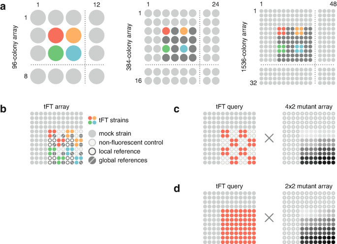
Different layouts of colony arrays. (a) Steps for assembling an array in 1536-colony format. In this example, a 96-colony array (12 × 8 columns and rows, left) is combined with three other 96-colony arrays (dark gray) in 384-colony format (24 × 16, middle). The 1536-colony array (48 × 32, right) is then assembled by pinning the 384-colony array four times, such that each strain is present in four technical replicates. A mock strain at the border of the arrays is indicated in light gray. The position of four strains (red, orange, green, blue) throughout the process is highlighted. Only one corner of the arrays is shown for simplicity. (b) Array in 1536-colony format to examine protein turnover using a library of tFT strains. Each 4 × 4 group contains one tFT strain in six technical replicates or in two biological replicates with three technical replicates each. A local reference strain and a non-fluorescent control are present throughout the array to locally correct fluorescence measurements for spatial effects and background fluorescence. Global reference strains should be included to normalize the data across multiple array plates. (c, d) Arrays in 1536-colony format to examine the turnover of a single tFT query in a library of mutants. Only one corner of the arrays is shown for simplicity. Layout of an array with a tFT query and a non-fluorescent control for background correction (c, left). Using SGA , the tFT query array is crossed with an array of mutants, each present in eight replicates in a 4 × 2 group. Layout of an array only with a tFT query (d, left). Using SGA , the tFT query array is crossed with an array of mutants, each present in four replicates in a 2 × 2 group

References
Balch WE, Morimoto RI, Dillin A, Kelly JW (2008) Adapting proteostasis for disease intervention. Science 319:916–919
Balchin D, Hayer-Hartl M, Hartl FU (2016) In vivo aspects of protein folding and quality control. Science 353:aac4354
Wolff S, Weissman JS, Dillin A (2014) Differential scales of protein quality control. Cell 157:52–64
Labbadia J, Morimoto RI (2015) The biology of proteostasis in aging and disease. Annu Rev Biochem 84:435–464
Khmelinskii A, Keller PJ, Bartosik A et al (2012) Tandem fluorescent protein timers for in vivo analysis of protein dynamics. Nat Biotechnol 30:708–714
Malínská K, Malínský J, Opekarová M, Tanner W (2003) Visualization of protein compartmentation within the plasma membrane of living yeast cells. Mol Biol Cell 14:4427–4436
Khmelinskii A, Meurer M, Ho CT et al (2016) Incomplete proteasomal degradation of green fluorescent proteins in the context of tandem fluorescent protein timers. Mol Biol Cell 27:360–370
Bachmair A, Finley D, Varshavsky A (1986) In vivo half-life of a protein is a function of its amino-terminal residue. Science 234:179–186
Bachmair A, Varshavsky A (1989) The degradation signal in a short-lived protein. Cell 56:1019–1032
Varshavsky A (2019) N-degron and C-degron pathways of protein degradation. Proc Natl Acad Sci U S A 116:358–366
Pédelacq J-D, Cabantous S, Tran T et al (2006) Engineering and characterization of a superfolder green fluorescent protein. Nat Biotechnol 24:79–88
Donà E, Barry JD, Valentin G et al (2013) Directional tissue migration through a self-generated chemokine gradient. Nature 503:285–289
Revenu C, Streichan S, Donà E et al (2014) Quantitative cell polarity imaging defines leader-to-follower transitions during collective migration and the key role of microtubule-dependent adherens junction formation. Development 141:1282–1291
Zhang H, Linster E, Gannon L et al (2019) Tandem fluorescent protein timers for noninvasive relative protein lifetime measurement in plants. Plant Physiol 180:718–731
Alber AB, Paquet ER, Biserni M et al (2018) Single live cell monitoring of protein turnover reveals intercellular variability and cell-cycle dependence of degradation rates. Mol Cell 71:1079–1091.e9
Durrieu L, Kirrmaier D, Schneidt T et al (2018) Bicoid gradient formation mechanism and dynamics revealed by protein lifetime analysis. Mol Syst Biol 14:e8355
Castells-Ballester J, Zatorska E, Meurer M et al (2018) Monitoring protein dynamics in protein O-mannosyltransferase mutants in vivo by tandem fluorescent protein timers. Molecules 23:2622
Devarajan S, Meurer M, van Roermund CWT et al (1862) Proteasome-dependent protein quality control of the peroxisomal membrane protein Pxa1p. Biochim Biophys Acta Biomembr 2020:183342
Khmelinskii A, Blaszczak E, Pantazopoulou M et al (2014) Protein quality control at the inner nuclear membrane. Nature 516:410–413
Kowalski L, Bragoszewski P, Khmelinskii A et al (2018) Determinants of the cytosolic turnover of mitochondrial intermembrane space proteins. BMC Biol 16:66
Meitinger F, Khmelinskii A, Morlot S et al (2014) A memory system of negative polarity cues prevents replicative aging. Cell 159:1056–1069
Dederer V, Khmelinskii A, Huhn AG et al (2019) Cooperation of mitochondrial and ER factors in quality control of tail-anchored proteins. elife 8:e45506
Kats I, Khmelinskii A, Kschonsak M et al (2018) Mapping degradation signals and pathways in a eukaryotic N-terminome. Mol Cell 70:488–501.e5
Shaner NC, Lambert GG, Chammas A et al (2013) A bright monomeric green fluorescent protein derived from Branchiostoma lanceolatum. Nat Methods 10:407–409
Shaner NC, Campbell RE, Steinbach PA et al (2004) Improved monomeric red, orange and yellow fluorescent proteins derived from Discosoma sp. red fluorescent protein. Nat Biotechnol 22:1567–1572
Bindels DS, Haarbosch L, van Weeren L et al (2017) mScarlet: a bright monomeric red fluorescent protein for cellular imaging. Nat Methods 14:53–56
Meurer M, Duan Y, Sass E et al (2018) Genome-wide C-SWAT library for high-throughput yeast genome tagging. Nat Methods 15:598–600
Janke C, Magiera MM, Rathfelder N et al (2004) A versatile toolbox for PCR-based tagging of yeast genes: new fluorescent proteins, more markers and promoter substitution cassettes. Yeast 21:947–962
Knop M, Siegers K, Pereira G et al (1999) Epitope tagging of yeast genes using a PCR-based strategy: more tags and improved practical routines. Yeast 15:963–972
Yofe I, Weill U, Meurer M et al (2016) One library to make them all: streamlining the creation of yeast libraries via a SWAp-tag strategy. Nat Methods 13:371–378
Baryshnikova A, Costanzo M, Kim Y et al (2010) Quantitative analysis of fitness and genetic interactions in yeast on a genome scale. Nat Methods 7:1017–1024
Weill U, Yofe I, Sass E et al (2018) Genome-wide SWAp-tag yeast libraries for proteome exploration. Nat Methods 15:617–622
Tong AH, Evangelista M, Parsons AB et al (2001) Systematic genetic analysis with ordered arrays of yeast deletion mutants. Science 294:2364–2368
Baryshnikova A, Costanzo M, Dixon S et al (2010) Synthetic genetic array (SGA) analysis in Saccharomyces cerevisiae and Schizosaccharomyces pombe. Methods Enzymol 470:145–179
Sherman F (1991) Getting started with yeast. Methods Enzymol 194:3–21
Winzeler EA, Shoemaker DD, Astromoff A et al (1999) Functional characterization of the S. cerevisiae genome by gene deletion and parallel analysis. Science 285:901–906
Wagih O, Parts L (2014) Gitter: a robust and accurate method for quantification of colony sizes from plate images. G3 (Bethesda) 4:547–552
Loader C (2013) Locfit: local regression, likelihood and density estimation. https://cran.r-project.org/package=locfit
R Core Team (2020) R: A language and environment for statistical computing. https://www.r-project.org/
Ghaemmaghami S, Huh W-K, Bower K et al (2003) Global analysis of protein expression in yeast. Nature 425:737–741
Huh W-K, Falvo JV, Gerke LC et al (2003) Global analysis of protein localization in budding yeast. Nature 425:686–691
Eldeeb MA, Siva-Piragasam R, Ragheb MA et al (2019) A molecular toolbox for studying protein degradation in mammalian cells. J Neurochem 151:520–533
Trauth J, Scheffer J, Hasenjäger S, Taxis C (2020) Strategies to investigate protein turnover with fluorescent protein reporters in eukaryotic organisms. AIMS Biophys 7:90–118
Čáp M, Štěpánek L, Harant K et al (2012) Cell differentiation within a yeast colony: metabolic and regulatory parallels with a tumor-affected organism. Mol Cell 46:436–448
Prakash S, Tian L, Ratliff KS et al (2004) An unstructured initiation site is required for efficient proteasome-mediated degradation. Nat Struct Mol Biol 11:830–837
Acknowledgments
We thank Balca Mardin for comments and acknowledge support from the European Research Council (ERC-2017-STG#759427 to A.K.).
Author information
Authors and Affiliations
Corresponding author
Editor information
Editors and Affiliations
Rights and permissions
Open Access This chapter is licensed under the terms of the Creative Commons Attribution 4.0 International License (http://creativecommons.org/licenses/by/4.0/), which permits use, sharing, adaptation, distribution and reproduction in any medium or format, as long as you give appropriate credit to the original author(s) and the source, provide a link to the Creative Commons license and indicate if changes were made.
The images or other third party material in this chapter are included in the chapter's Creative Commons license, unless indicated otherwise in a credit line to the material. If material is not included in the chapter's Creative Commons license and your intended use is not permitted by statutory regulation or exceeds the permitted use, you will need to obtain permission directly from the copyright holder.
Copyright information
© 2022 The Author(s)
About this protocol

Cite this protocol
Fung, J.J., Blöcher-Juárez, K., Khmelinskii, A. (2022). High-Throughput Analysis of Protein Turnover with Tandem Fluorescent Protein Timers. In: Pérez-Torrado, R. (eds) The Unfolded Protein Response. Methods in Molecular Biology, vol 2378. Humana, New York, NY. https://doi.org/10.1007/978-1-0716-1732-8_6
Download citation
DOI: https://doi.org/10.1007/978-1-0716-1732-8_6
Published:
Publisher Name: Humana, New York, NY
Print ISBN: 978-1-0716-1731-1
Online ISBN: 978-1-0716-1732-8
eBook Packages: Springer Protocols