Article

An Assessment of Stratospheric Intrusions in Italian Mountain Regions Using STEFLUX

1
Institute of Atmospheric Sciences and Climate, National Research Council of Italy, 40129 Bologna, Italy
2
Department of Psychological, Health & Territorial Sciences, University “G. d’Annunzio” of Chieti-Pescara, 66100 Chieti, Italy
3
RSE S.p.A.—Ricerca sul Sistema Energetico, Via Rubattino, 20134 Milano, Italy
4
Institute of Atmospheric Pollution, National Research Council of Italy, 87036 Rende, Italy
*
Author to whom correspondence should be addressed.
Atmosphere 2018, 9(10), 413; https://doi.org/10.3390/atmos9100413
Submission received: 18 September 2018 / Revised: 15 October 2018 / Accepted: 16 October 2018 / Published: 22 October 2018
(This article belongs to the Special Issue Stratosphere–Troposphere Exchanges)

Abstract

:
The Mediterranean basin is considered a global hot-spot region for climate change and air quality, especially concerning summer-time ozone (O3). Previous investigations indicated that the Mediterranean basin is a preferred region for stratosphere-to-troposphere exchange (STE) and deep stratospheric intrusion (SI) events. The Lagrangian tool STEFLUX, based on a STE climatology that uses the ERA Interim data, was hereby used to diagnose the occurrence of deep SI events in four mountain regions over the Italian peninsula, spanning from the Alpine region to the southern Apennines. By using near-surface O3 and relative humidity (RH) observations at three high-mountain observatories, we investigated the performance of STEFLUX in detecting deep SI events. Both experimental and STEFLUX detections agreed in describing the seasonal cycle of SI occurrence. Moreover, STEFLUX showed skills in detecting “long-lasting” SI events, especially in the Alps and in the northern Apennines. By using STEFLUX, we found positive tendencies in the SI occurrence during 1979–2017. However, in contrast to similar studies carried out in the Alpine region, the negative long-term (1996–2016) trend of O3 in the northern Apennines did not appear to be related to the SI’s variability.

1. Introduction

The Mediterranean basin is considered a global hot-spot region for climate change [1] and air-quality [2]. In particular, tropospheric ozone (O3) is a well-known, short-lived climate forcer and pollutant, which, besides playing a role on regional climate, can have adverse effects on population health and ecosystems [3]. Indeed, the importance of O3 lies in its capability to absorb long-wave radiation emitted by the Earth’s surface and act as a powerful oxidizing agent that can determine the overall oxidative capacity of the troposphere. Due to its high oxidizing capacity, it can cause serious health problems, especially respiratory illnesses and cardiovascular diseases, leading to premature death in some cases. It also damages vegetation such as forests and agricultural crops and the services they provide, in particular biomass production and carbon sequestration [4].
Meteorological conditions such as frequent clear sky and high solar radiation in summer enhance the formation of photochemical O3, due to the availability of natural and anthropogenic precursors. Modeling scenarios and satellite investigations indicate the central Mediterranean basin (i.e., from 5° E to 20° E) as the region where near-surface O3 is maximized in summer [5,6]. Moreover, the Mediterranean basin was identified by previous studies (e.g., [7,8]) as a favorable region where stratosphere-to-troposphere exchange (STE) can affect the troposphere chemistry down to the planetary boundary layer (PBL), possibly contributing to enhanced O3 levels (e.g., [9]). Indeed, the Mediterranean basin is located just southward of the typical position of the polar front jet, and the Alpine lee-cyclogenesis can further favor the occurrence of STE [10].
In the 2012–2018 period, one aim of the Project of Interest NextData (www.nextdataproject.it) was to investigate the processes influencing the variability of pollutants and climate-altering compounds in mountain ecosystems in Italy, to support impact studies on mountain environments. Special attention was devoted to investigating the impact of stratospheric intrusions (i.e., the transport of stratospheric air masses deep into the troposphere associated with synoptic-scale atmospheric variability) on near-surface O3 in mountain regions. In this framework, the Stratosphere-to-Troposphere Exchange Flux (STEFLUX) tool [11] was developed as an easy and fast-to-use instrument to diagnose the occurrence of stratospheric intrusions (SIs) in specific regions on the Earth’s surface or within tropospheric columnar domains. A test application at two locations (Himalayas and central Apennines) suggested good ability in reproducing SI seasonality and satisfactory skill in identifying specific SI events [
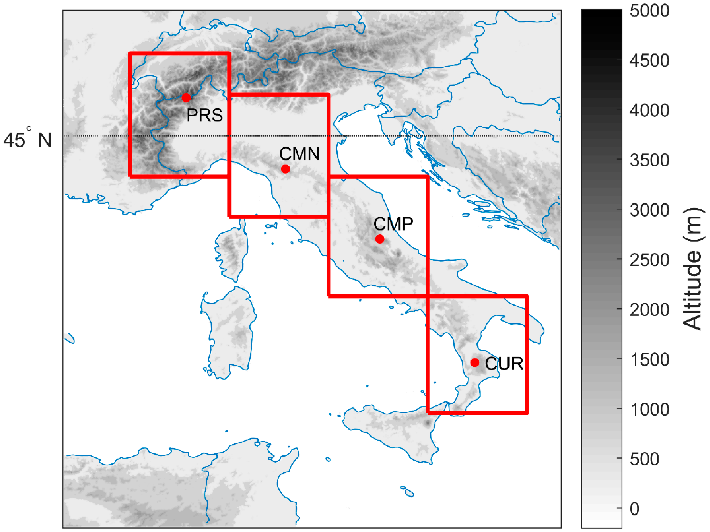
11]. In the framework of NextData, a long-term (1979–2017) dataset of SI occurrence was produced for four high-mountain regions in Italy (western Alps, northern, central, and southern Apennines), where permanent atmospheric observatories are located (Plateau Rosa—3480 m a.s.l., Mt. Cimone—2165 m a.s.l., Mt. Portella—2401 m a.s.l., and Mt. Curcio—1796 m a.s.l., see Figure 1).
In this work, we will present and discuss these long-term datasets. The availability of continuous observations of atmospheric variables at three of these high-mountain measurement sites (Plateau Rosa, Mt. Cimone, and Mt. Curcio), provides the opportunity to further extend the evaluation of STEFLUX ability to diagnose the occurrence of SI events over these regions, which span more than 7° in latitude and 1500 m in altitude over the Italian territory.
Many past studies made use of observations of “stratospheric tracers” (i.e., O3, RH, and radiotracers) at high-mountain sites for investigating STE [12,13,14,15,16,17]. Indeed, as being less influenced by polluted air masses with respect to locations at lower altitudes or within the PBL, SI detection at high-mountain sites is more straightforward. However, the ability to detect the occurrence of stratospheric air masses in the troposphere is limited by air mass mixing and dilution [18,19] due to turbulence [20] or convective activity [21,22]. Nevertheless, Trickl et al. [17] suggested that, without strong wind shear or convective processes, the mixing of descending stratospheric air in the troposphere is slow and mostly limited to the boundaries of the stratospheric layers. This would make atmospheric chemistry observations at high-mountain measurement sites even more reliable at detecting SI occurrence.
The manuscript is structured in the following way. In Section 2 we describe the high-mountain measurement sites, together with the instrumentation and methodologies used to detect the occurrence of SI events from near-surface observations. In this Section the STEFLUX tool is also described. Section 3 provides results about the SI identification at the different mountain sites, together with a comparison with STEFLUX outputs, to evaluate the ability of STEFLUX to diagnose the occurrence of SI in these regions. Then, by using STEFLUX, we also provide long-term SI climatology (1979–2017) for these observatories. The discussion of the results and possible implication for near-surface O3 variability is given in Section 4, while conclusions are presented in Section 5.

2. Experiments

2.1. In Situ Observations at High-Mountain Observatories

In this study, daily SI occurrences were derived for four high-mountain regions in Italy (see Figure 1). Unfortunately, experimental problems prevented one obtaining an extended dataset for O3 and RH observations at Mt. Portella–Campo Imperatore (central Apennines). Thus, the STEFLUX performance assessment was carried out using data from Plateau Rosa (western Alps), Mt. Cimone (northern Apennines), and Mt. Curcio (southern Apennines) only. In the following, we will provide a brief description of the measurement sites included in the assessment, together with the suite of atmospheric observations used in this study. More detailed metadata information can be found at https://geonetwork.igg.cnr.it.
Plateau Rosa (PRS, 45.93° N, 7.70° E, 3480 m a.s.l.) is a WMO/GAW regional station, located in the Italian Alps of the Aosta Valley, on the southern ridge of Teodulo hill, in the municipality of Valtournenche. The area in the vicinity of the measurement site is characterized by snowfields and glaciers and is far from urban and industrialized districts. The closest urban/industrialized area is Aosta (nearly 35,000 inhabitants), placed 30 km away. More industrialized centers such as Turin (900,000 inhabitants) or Milan (1.3 million inhabitants) are located 100 km south-west and 132 km south-east of PRS, respectively. Continuous measurements of surface O3 are performed at PRS by using an UV-absorption analyzer (Thermo 49i). Measurements were started in 2006, but some gaps in the time series occurred, which led to 87% of data availability. The RH observations used in this study only cover the period 2012–2017.
Mt. Cimone (CMN, 44.19° N, 10.70° E, 2165 m a.s.l.) is the only WMO/GAW global station in Italy. Being the highest peak of the Italian northern Apennines, the observations carried out at CMN can be considered representative of the background conditions of the troposphere for most of the year, although during warm periods the station can be affected by thermal and convective transport of PBL air. Furthermore, only small villages are present in the proximity of the station. The closest village is Sestola (1500 inhabitants), located 15 km far from the site; the closest urban and industrialized areas are Florence, Modena, and Bologna, all within a radius of 50–60 km from CMN. O3 measurements, active since 1996 adopting the UV-absorption technique, are performed with a Dasibi 1108 W/GEN (1996–2015) and a Thermo 49i (2016–onward). Over the whole measurement period, RH was observed with capacitive sensors by Rotronics. More details about CMN can be found in Cristofanelli et al. [23].
Mt. Portella–Campo Imperatore (CMP, 42.45° N, 13.55° E, 2401 m a.s.l.) is located inside the National Park of Abruzzo, on the crest of Mt. Portella. The area in the immediate vicinity of the measurement site is characterized by rocky outcrops and grasslands, which are completely covered by snow in winter. With the exception of a mountain hut (200 m east from the site), there are no buildings within a radius of 2 km. The biggest close municipality is L’Aquila (60,000 inhabitants), placed 16 km to the south of CMP. Over July 2012–November 2014, O3 measurements were performed with a UV-absorption analyzer (2B Technologies, model 205), while since August 2015 the station was equipped with a Thermo 49i. Meteorological observations are carried out by an integrated weather station Vaisala WXT520. Unfortunately, several extended data gaps, due to damages from lightning and prolonged lack of power during the snow period, affected CMP data, thus preventing the completeness of a continuous time series.
Mt. Curcio (CUR, 39.31° N, 16.42° E, 1796 m a.s.l.) is a WMO/GAW regional station, located in a strategic and isolated position within the Sila National Park in the Italian southern Apennines. The station is characterized by no local sources of contamination and no road access. Being placed 200 m from the cable car arrival of the near ski resort, CUR has a completely free horizon, allowing one to carry out atmospheric monitoring measurements with a large degree of spatial representativeness. The station is placed in the middle of the Mediterranean basin, around 30 and 60 km from the Tyrrhenian and the Ionian seas, respectively. At CUR, atmospheric observations started in 2015, in the framework of the PON I-AMICA Project (www.i-amica.it). O3 measurements are performed using a Teledyne API 400A UV-absorption analyzer. Meteorological parameters are monitored using the LSI LASTEM integrated weather station, with RH measurements performed by a thermo-hygrometer DMA875. For the comparison with STEFLUX, we restricted the observation period to January 2015–June 2016, when O3 and RH observations were available.
At these measurement sites, near-surface O3 measurements are performed by adopting the standard operation procedures recommended by WMO/GAW [24]. Automatic zero and span checks are executed every 24–48 h using activated charcoal cartridges and internal UV O3 sources. Multi-point calibrations against laboratory standards linked to the reference scale SRP#15 hosted at the WMO/GAW “World Calibration Center for surface O3, Carbon Monoxide and Methane” hosted at EMPA (Dübendorf, Switzerland) are carried out every 3–12 months. Extended uncertainty (coverage factor k = 2) was usually lower than 1 ppb for O3 measurements in the range 0–100 ppb.

2.2. SI Identification at Mountain Sites

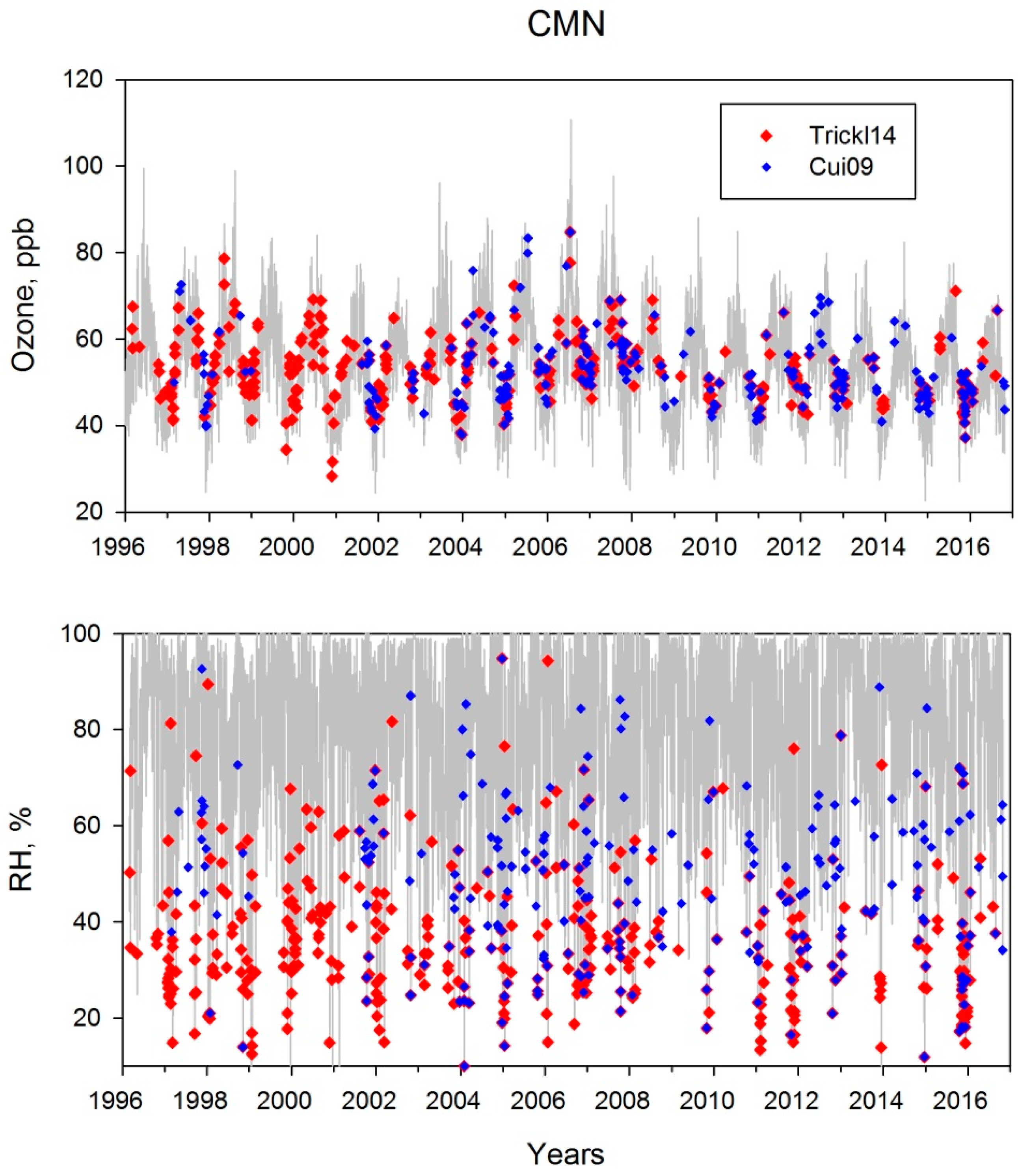
To assess the STEFLUX performance in identifying time periods affected by SI at the mountain observatories, we analyzed near-surface O3 and RH, which are widely used as tracers for stratospheric air masses in the troposphere [10,11,12,14]. Indeed, stratospheric air masses are usually characterized by higher O3 content and lower water vapor than tropospheric air. According to Cui et al. [14], if hourly O3 values were continuously higher than the 10-day running mean by 10% and RH values were below 50% for a time period of at least 6 h, SI events were identified by measurements. We defined this approach as “Cui09” criterion. Because a fraction of days was characterized by the lack of simultaneous O3 and RH measurements at CMP and CUR, we also considered a detection algorithm that considers only RH. As suggested by Trickl et al. [17], to identify stratospheric air from near-surface observations at a mountain site, a RH threshold of 30% can be considered adequate [15,25]. Thus, following Trickl et al. [17], if observed hourly RH values were lower than 30% within ±6 h, a SI event was identified (hereinafter, “Trickl14” criterion). Even if other identification criteria were proposed by other studies [10,11,12,14,15], we decided to make use of these selection criteria (“Cui09” and “Trickl14”) due to their high feasibility, which made the obtained results easily reproducible, and due to their relatively high reliability in detecting SI at high-mountain sites (see [12,15,17]). Moreover, these criteria are based on atmospheric parameters simultaneously observed at the considered measurement sites, thus not introducing (or limiting) possible biases among the sites due to different selection methodologies. Again, these criteria are only based on pure observational data, which is advisable for the comparison with a modeling tool based on a meteorological reanalysis dataset.

2.3. STEFLUX

The Stratosphere-to-Troposphere Exchange Flux (STEFLUX, see [11]) tool is a fast-computing and reliable methodology with which to detect SI events at a specific location and during a user-defined time window. It is based on the trajectories from the STE climatology presented in Škerlak et al. [8], which makes use of the ERA-Interim reanalysis dataset [26] from the European Centre for Medium-Range Weather Forecasts (ECMWF) for calculating mass and ozone fluxes across the tropopause and several surface pressures. The trajectories are computed using the 3-D wind fields from ERA-Interim on a regular grid, with horizontal spacing of approximately 80 km, and 30 hPa in the vertical (except for tropical trajectories, where the spacing is 10 hPa due to the typically slower vertical motion). Each trajectory that crosses the tropopause (defined as the 2 pvu/380 K barrier) in the first 24 h is selected and then extended backward and forward in time, to create a 9-day long trajectory. Furthermore, a 3-D labelling algorithm is applied to avoid “false” detections [8].
The STE trajectories are processed by STEFLUX, and the ones that originated in the stratosphere and crossing a tropospheric 3-D target box, during a specific time window, are detected. The extension of the box (horizontal boundaries and top lid) and the time window are the parameters that can be varied by the user, as well as the temporal resolution for the STE trajectories (i.e., from 6 h, the default value, up to 1 h). Several output files are produced by STEFLUX: (i) the trajectory positions and timing within the box, (ii) the first box crossing positions and timing for each trajectory, (iii) the tropopause crossing locations and timing for each trajectory, and (iv) the complete ensemble of trajectories that have crossed the box. The availability of the ERA-Interim input data allows one to compute long-term climatology of SI events at each site, since data extend back to 1979.
The first systematic comparison with SI detection from two high-mountain sites in Italy and Himalayas suggested that STEFLUX correctly represented the typical seasonal cycles of SI frequencies and was able to detect single events with a duration longer than 1 day, thus being useful for determining the SI events occurring on a regional scale [11].

2.4. SI Identification by STEFLUX

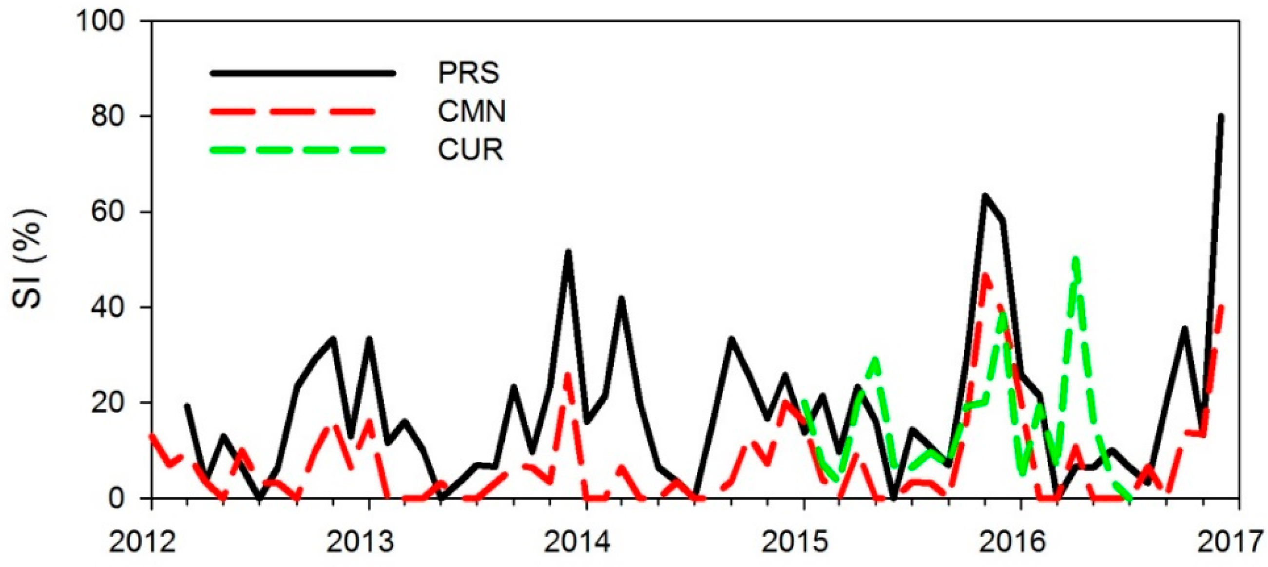
To compare STEFLUX outputs with near-surface observations at PRS, CMN, and CUR, the model was run for three target areas with several input configurations, allowing one to perform sensitivity tests on the different configuration parameters. Considering all the possible configurations deployed, the horizontal boxes spanned from 1° × 1° to 3° × 3° around each station, and the vertical extensions were chosen as the typical average pressure level recorded at each site, together with ±50 hPa. The selected time periods correspond to those reported in Section 2.1 and Table 1. The temporal resolution for the STE trajectories was chosen as 1 point every hour. For all the measurement sites, the STEFLUX detection over the target box with extension 3° × 3° and the top lid overlapping the average pressure levels of the measurement sites (i.e., 660 hPa for PRS, 790 hPa for CMN, and 820 hPa for CUR) will be shown in the paper. This choice was determined by a preliminary sensitivity test based on the comparison between STEFLUX outputs with different configurations and the in situ SI identification by “Cui09” and “Trickl14” (see Table S1 in the Supplementary Material for a summary of the comparison). It must be argued that the target regions for which STEFLUX showed the best agreement with in situ SI detection encompassed very large spatial regions extending well beyond the mountain regions object of the experiment (see Figure 1). Nevertheless, it must be kept in mind that STEFLUX should not be regarded as a tool for exactly reproducing SI occurrences at specific measurement sites, which are typically strongly affected by rather small-scale circulations. Indeed, as stated in Putero et al. [11], its best application is the determination of SI inputs on a regional scale. It is thus reasonable that the best agreement between experimental in situ detection and STEFLUX outputs is found by inspecting a rather large domain around the mountain region of interest.

3. Results

3.1. Comparison between In Situ SI Identification and STEFLUX

To obtain a statistical evaluation of the STEFLUX ability to reproduce SIs at the high-mountain sites considered in this study, we compared the results of in situ SI identification (Section 2.2) with the STEFLUX outputs (Section 2.3). As an example, Figure 2 reports O3 and RH observations at CMN from 1996 to 2016, together with days identified as affected by SI according to “Cui09” (red points) and “Trickl14” (blue points). The same plots for PRS and CUR can be found in the Supplementary Material (Figures S1 and S2).
Table 2 reports the total frequency of detected SI for each measurement site, as a function of the identification criteria. Also reported in the Table is the “all detections” column, i.e., the SI identification by any of the two criteria. Depending on the measurement sites, the “Trickl14” criterion estimated from 45% (at PRS) to 75% (at CUR) more detection than the “Cui09” criterion. The highest SI occurrences were diagnosed for PRS and CUR, while a lower SI frequency was diagnosed for CMN. Concerning STEFLUX, an overestimation of the number of days affected by SI events can be observed for PRS and CMN (+40%), while an underestimation (−30%) is observed for CUR. By considering only the short period for which O3 and RH data are available at CUR, the STEFLUX overestimation is still confirmed at PRS but significantly reduced for CMN (+13%). This would suggest that, due to the short period of investigation, particular attention must be devoted to generalizing results from CUR observations.
For all the measurement sites, the seasonal cycle of SI detection is characterized by clear variability, with the highest occurrence in winter and minima in summer (Figure 3, left). This seasonal cycle is enhanced for CMN, where SI occurrences in winter/late autumn (up to 12–14%) were 6–7 times higher than in summer (about 2%). At CUR, the southernmost station, a peak was evident in spring, with the SI occurrence (“Trickl14”) approaching the peak value observed in December. Additionally, for PRS, the highest occurrence of SI was found in December. STEFLUX indicated a clear seasonal cycle in the monthly SI frequency (Figure 3, right), which is rather consistent with in situ SI detection. For PRS, STEFLUX nicely reproduced the summer minimum and the autumn increase of SI frequency, but clearly overestimated (by more than a factor of 2) the SI occurrence in winter-spring: this is the reason of the overall overestimation of STEFLUX detection at PRS. The CMN seasonal cycle is more consistent between STEFLUX and in situ SI detection, with a high overestimation only in spring and a small overestimation in winter. Despite the two “northern” stations, for CUR we observed better agreement from January to June between STEFLUX and observations. In particular, STEFLUX nicely reproduced the spring peak observed at CUR and the secondary peaks in late winter and autumn. On the other hand, STEFLUX completely missed the large peak in December seen by the “Trickl14” criterion. This peak in SI frequency was related to the occurrence of five short (i.e., less than three days) SI events at CUR, which was not captured by the model.
To obtain more hints about the seasonal behavior of SI occurrence at the three measurement sites, in Figure 4 we plotted the time series of monthly SI frequency (by considering all the detection criteria) for the period of common data availability (i.e., 2012–2016). It is evident that the spring peak at CUR was driven by very high SI occurrence in April 2016, while the presence of a large December peak (frequency >40%) is an almost systematic feature at PRS that occurred on 2013, 2015, and 2016. It is interesting to note that these months also represented the peaks in SI frequency at CMN (>20%), thus suggesting a common origin for this feature, which affected the Alpine and Apennine regions. Additionally, on November 2015, a large frequency of SI occurrence was diagnosed for PRS and CMN. To assess the ability of STEFLUX in reproducing the interannual variability of seasonal SI frequency, we calculated the Pearson correlation coefficient between STEFLUX and in situ SI frequency for PRS and CMN. A high correlation coefficient (r = 0.64) was found for PRS, while a moderate correlation (but significant at the 95% confidence level) was found for CMN (r = 0.46).
The identification of specific SI events still represents a very difficult task for atmospheric models [11,14]. As done in Putero et al. [11], a SI event is hereby defined as the aggregation of contiguous SI days identified by one of the methodologies (i.e., “Cui09” and “Trickl14”, or STEFLUX). Cases in which two distinct SI events are separated by a single no-SI day are treated like a unique SI event covering the entire period. To evaluate the STEFLUX ability in detecting single SI events diagnosed by in situ observations (i.e., “Cui09” and “Trickl14”) at PRS, CMN, and CUR, we adopted the approach proposed by Cui et al. [14] and already used in Putero et al. [11]. We considered the SI events detected by the in situ methodologies, and we checked if also STEFLUX provided evidence for SI occurrence during the same temporal frame. The results are reported in Table 3. For PRS, STEFLUX was able to confirm 49% of the SI events detected by measurements. The best agreement (from 62% to 83%) was found for “long-lasting” events (i.e., with a duration longer than three days), while the “hit score” decreased for shorter events (about 37%). The percentage of agreement was lower for CMN (total: 23%). Similarly to PRS, the best agreement was found for long-lasting events (>4 days) but, in contrast to PRS, it was not possible to find out a monotonic tendency of STEFLUX performance with event duration, i.e., a satisfactory performance was observed for events with length up to 2 days (23%), but a decrease of the “hit score” appeared for 3-day long events. The situation was even worse for CUR: STEFLUX, which was able to catch only 11% of SI detected by in situ measurements. For PRS and CMN, STEFLUX is able to identify long and medium SI events, but the detection ability strongly decreases for short events. These results agree with previous assessments of ability of Lagrangian model to systematically detect single SI events [11,14]. The bad agreement between CUR observations and STEFLUX outputs, even considering the rather short period of comparison, can suggest a decrease of STEFLUX performances with decreasing latitudes.

3.2. STEFLUX Long-Term Climatology

By considering the STEFLUX configurations summarized in Table 1, we exploited the feature of STEFLUX of extending calculations back to 1979, since this is the temporal extension that can be found in the ERA-Interim reanalysis data. Therefore, we expanded calculations for all sites to 1979–2017, to have a long-term climatology of SI events for each region considered. Even if we were not able to perform a comparison for CMP, we considered the climatology also for this measurement site, setting-up the top lid of the target box to the average pressure of the station (i.e., 760 hPa) and the horizontal extension to a 3° × 3° area around the site location, in agreement with the configuration for other sites (Table 1). As shown in Section 3.1, STEFLUX had a better agreement (particularly for PRS and CMN) in identifying SI events longer than three days. For this reason, we carried out two climatological studies in parallel, i.e., annual frequencies of SI occurrence considering: (i) all of the SI events detected by STEFLUX and (ii) only the days that constitute a “long” event (i.e., longer than three days), for which STEFLUX demonstrated more robust skill in identifying specific events.
Figure 5 shows the trend analysis for the four measurement stations, carried out on annual SI frequency values; trends were calculated by using the Theil-Sen [27,28] regression method available in Openair software [29]. CMN showed a significant (p < 0.05) increasing trend of 0.08% yr−1 considering all SI events; this trend was not significant when the analysis was limited to long events. PRS showed no difference among the two categories of events (i.e., 0.07% yr−1), although none of these trends is statistically significant. A statistically significant (p < 0.1) increasing trend was found for PRS when considering spring values only, for long events, i.e., 0.31% yr−1 (see Table S1 in the Supplementary Material). CMP presented an analogous trend (0.09% yr−1) for the two time series, which was statistically significant in both cases (p < 0.1). As for PRS, a significant (p < 0.1) increasing trend (0.16% yr−1) was also found for spring frequencies computed on all SI values. For CUR, the spread in the frequency values between all and long events was wider than the other stations, likely indicating that this site is largely interested by “short” (i.e., shorter than three days) events. Interestingly, the significant trend (p < 0.1) was found only for long events (i.e., 0.05 yr−1).
The annual variations computed using these climatological datasets are shown in Figure 6. The box-and-whisker plots consider all of the SI events, while the average annual variation is reported both for all and “long” events. The annual variation was similar for all of the sites, with an evident minimum in summer and maximum values in winter. This behavior, consistent also for long events, reflects what is shown in Figure 3 for CMN and PRS, over the shorter temporal periods. Interestingly, CUR shows a different cycle, thus indicating that the evident spring peak with maxima in April–May displayed in Figure 3 is probably due to a “transient” feature that occurred in 2015.

4. Discussion

In agreement with the previous results by Putero et al. [11], the present study indicated that STEFLUX provides a satisfactory representation of the typical seasonal cycles of SI occurrence over mountain regions in Italy. The comparison with PRS in situ detection revealed an overestimation of frequency during winter and spring. As showed by Škerlak et al. [8], the western Alpine region represents the southern boundary of a region characterized by a maximum of deep STE in winter (December–February). It is thus reasonable to assume that the relatively large target region (3° × 3°) adopted in this work can also select events that actually occurred northward or westward of PRS. To better assess this point, we calculated the monthly frequency of SI occurrence diagnosed by STEFLUX for PRS (2012–2016), considering a target box with 1° × 1° extension (Figure S3 in the Supplementary Material). With this configuration, a good agreement with in situ SI frequencies was obtained for January, April, and May (deviations within ±3%), while SI occurrence was overestimated (underestimated) by 9% (11%) for February (March). On the other hand, for July–December, the 1° × 1° configuration strongly underestimated (−68%) SI occurrences by in situ detection. This limitation must be considered when using STEFLUX results to discuss features or processes related to SI over these regions and, based on the current study, the 1° × 1° configuration appeared to be the most suitable to investigate SI occurrence over the Italian western Alpine regions in winter-spring. The seasonal cycles of SI frequency obtained by the near-surface observations and by STEFLUX at our Alpine and Apennines observatories are in nice agreement with Cristofanelli et al. [10] and Trickl et al. [15,17].
The identification of single SI events was more problematic: this further supports the already-evidenced limitation of the Lagrangian models in capturing SI events at the Earth’s surface, even at high-mountain sites [14,16,30]. Together with the systematic underestimation of seasonal SI occurrence in December, this led to a rather low rate of SI identification at the southernmost region of Italy. Once again, it must be stated that the relatively short period of continuous observations available at CUR would prevent any conclusive assessment about STEFLUX performance. Nevertheless, this preliminary assessment would suggest that the STEFLUX outputs should be treated with caution in the central Mediterranean basin. The reason for the underestimation of SI occurrence can be tentatively related to the ability of ERA-Interim to reproduce the transport of stratospheric air masses towards the lower troposphere of the central Mediterranean basin: for this region, meridional air mass transport can be particularly relevant for the presence of stratospheric air in the lower troposphere (STE usually occurred at more northern and western locations, see [8]). It is thus conceivable that the relatively coarse spatial resolution characterizing the ERA-Interim dataset (approximately 80 km) does not allow one to correctly reproduce the downward and meridional transport of air masses from the stratosphere. A further point of concern can be related to the representation of subgrid-scale processes (e.g., convection, turbulent diffusion, and mixing), which can play non-negligible roles in the vertical transport of air masses down to the PBL and Earth’s surface.
Once we had considered these caveats, we used the STEFLUX outputs to provide a systematic assessment of the possible SI contribution to the near-surface O3 variability observed at PRS, CMN, and CUR. Contradicting results exist regarding the impact of STE on O3 levels and variability in the lower troposphere, and the question of where and how often SIs can reach the PBL and to what extent STE contributes to O3 levels at the surface is a topic of ongoing research (e.g., [31] and references therein). To this aim, we analyzed the daily O3 values observed at our high-altitude measurement sites as a function of the occurrence of SI as diagnosed by STEFLUX. As a function of different seasons, Table 4 reports the average O3 values for days affected or not by SI. With the purpose of retaining only periods characterized by the presence of dry (stratospheric) air masses at the measurement sites, a further data selection was implemented by considering only days for which STEFLUX diagnosed SI but with daily average RH lower than 60%. For PRS, the same analysis was repeated by configuring STEFLUX with the 1° × 1° target area for January–July: the results were not significantly different from the ones reported in Table 4 (which refer to the 3° × 3° configuration). It has to be noted that, for specific seasons and data selections, not enough SI events were diagnosed by STEFLUX for CUR to make a statistical analysis possible. For all the measurement sites, a statistically significant O3 increase was found for SI days during winter, while it was not possible to find a univocal SI influence for the other seasons: a statistically significant O3 increase was found for SI days in spring (CUR), while an average O3 decrease was observed for CMN in spring and autumn. These results are in good qualitative agreement with a previous study by Cristofanelli et al. [10], who reported that, at CMN, the SI contribution to O3 was largest in winter.
Some authors (e.g., [13,15]) suggested the existence of long-term trends in the O3 flux from the stratosphere, able to influence O3 trends in the lower free troposphere over Europe. Figure 7 reports the long-term trend (1996–2017) of near-surface O3 at CMN, as calculated by the Theil-Sen regression. A significant (p < 0.01) decreasing trend of −0.20 ppb yr−1 was estimated, considering all the available O3 observations. If days affected by SI (as diagnosed by STEFLUX) were neglected in the trend analysis, a similar O3 trend was still obtained (−0.21 ppb yr−1). These results suggest that the overall negative O3 trend observed at CMN from 1996 to 2016 is not strongly influenced by SI variability. Finally, we analyzed the time series of O3 values for days affected by SI: a negative trend (−0.13 ppb yr−1) was obtained. Thus, even if the frequency of SI appeared to increase with time at CMN (Figure 5), the amount of O3 related to SI seemed to decrease. This negative tendency is evident also when SI days with RH < 60% are considered and, thus, appeared to be a robust feature in the SI time series. This evidence is in contrast with the results from Ordóñez et al. [13] and Trickl et al. [15,17], who indicated the existence of a positive trend of the stratospheric component for near-surface O3 record in the Alpine regions. However, it should be remembered that CMN is located in the Mediterranean basin and at lower altitudes with respect to the measurement sites considered in those works, as also indicated by the lower rate of SI occurrence with respect to PRS, which highlights the specific features of typical Mediterranean mountain locations with respect to the Alpine ones.

5. Conclusions

In this work, we investigated SI events over the Mediterranean basin by using near-surface observational data from high-mountain sites in Italy (spanning from the Alpine region to the southern Apennines) and model outputs using the Lagrangian tool STEFLUX. The comparison between near-surface observational SI and those identified with STEFLUX confirmed that this tool is able to represent the seasonal cycle of SI occurrence and can reasonably identify long-lasting (i.e., with a duration of at least three days) SI events, especially in the Alps and northern Apennines. Both near-surface observations and STEFLUX outputs indicated a clear seasonal cycle (higher frequency during cold months and lower frequency during summer) for the SI frequency, with much higher absolute frequencies for the western Alpine region (PRS) with respect to the Apennines (CMN, CMP, and CUR). This clearly suggests a decreasing “direct” influence of stratospheric input to the lowest troposphere, moving from the Alpine regions towards the heart of the central Mediterranean basin. The comparison with the experimental detection at PRS suggested that, for the western Alpine region, the STEFLUX configuration is optimized when the horizontal box extension is set to 1° × 1° for January–June and to 3° × 3° for July–December.
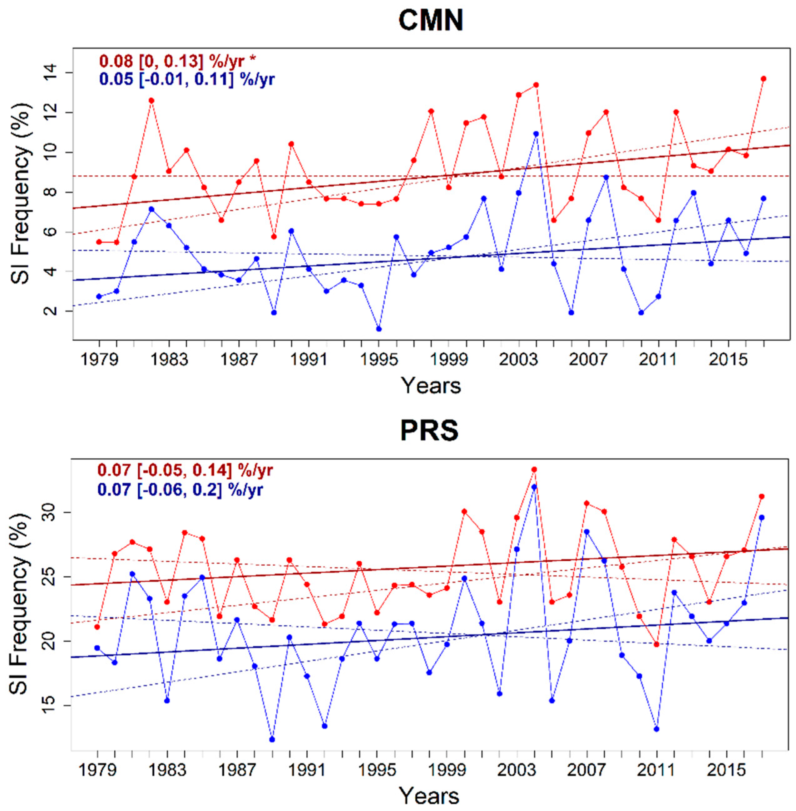
As being based on a global STE dataset derived from ERA-Interim, STEFLUX allowed one to produce a long-term climatology (1979–2017) of SI events for the investigated mountain regions. The calculated datasets can be obtained by NextData through the portal 
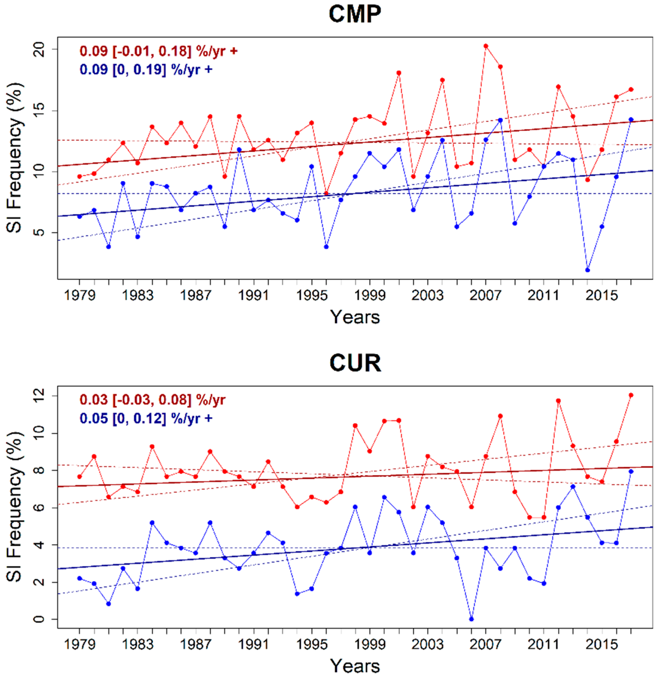
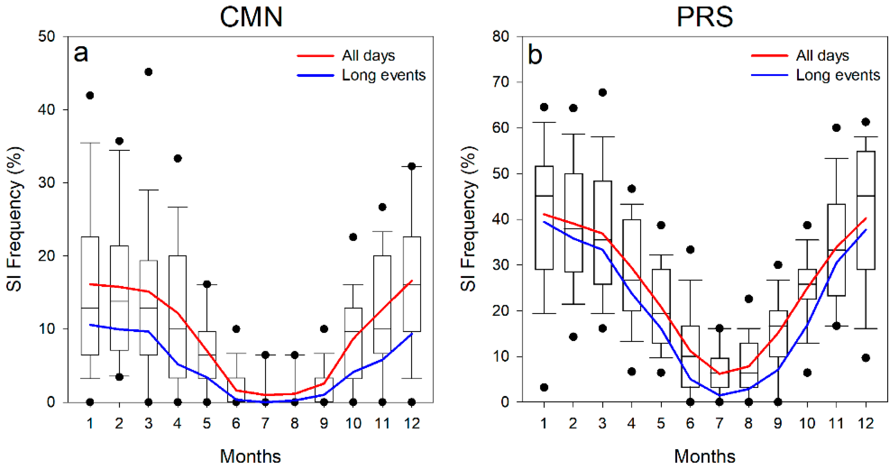
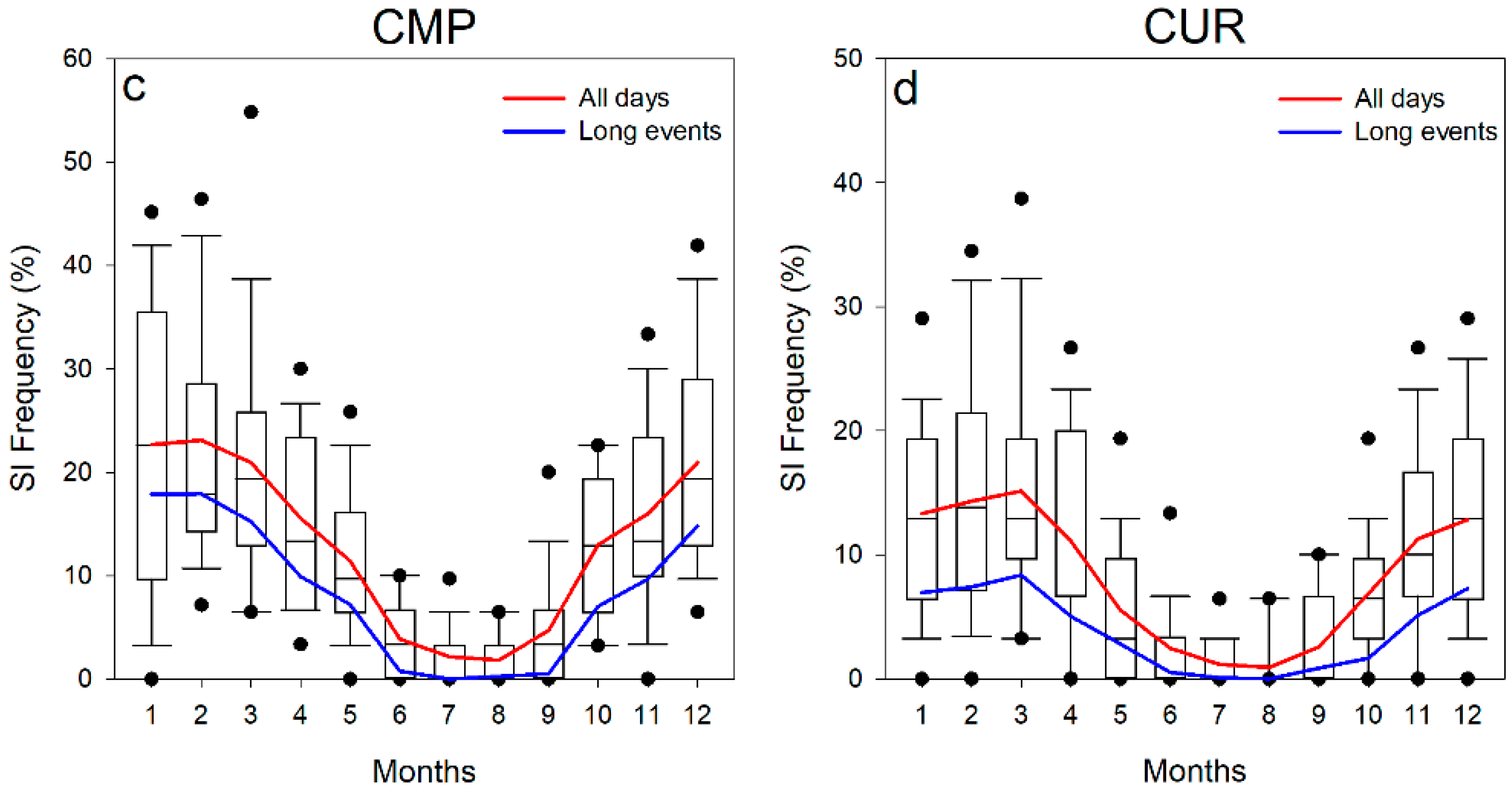
https://geonetwork.igg.cnr.it. For all of the measurement sites, the seasonal cycle of SI frequency over 1979–2017 resembles the one obtained from the experimental data, i.e., highest values during winter and minima during summer. The fraction of long-lasting vs. all events is about 60% for the stations in the Apennines (CMN, CMP, and CUR) and about 85% for PRS (which is located at a higher altitude). Interestingly, despite the other stations, a peak in SI frequency emerged for CUR (southern Apennines) in early spring (March). The analysis of long-term SI frequency (for both all events and long-lasting ones) revealed the existence of small positive tendencies for all the considered regions (from 0.03% yr−1 to 0.09% yr−1 for all and long-lasting SI events, respectively). These tendencies are statistically significant for CMN, CMP, and CUR. At the moment, we are not able to provide robust attribution for the appearance of these tendencies in SI frequency. More work will be carried out in the future to investigate the dynamical processes that are able to explain the causes of these tendencies.
Finally, we used STEFLUX for assessing the possible impact of SI to O3 variability at PRS, CMN, and CUR. For the periods in which O3 observations were available at PRS, CMN, and CUR, we found that, for the winter seasons, days affected by SI were characterized by higher O3 values, while no univocal signals were found for the remaining seasons. The statistical analysis of the long-term O3 (1996–2016) trend at CMN suggested that SIs are not a driving process for the appearance of the detected negative trend.

Supplementary Materials

The following are available online at https://www.mdpi.com/2073-4433/9/10/413/s1, Figure S1: measured O3 (top) and RH (bottom) daily values at PRS (grey lines). Red (blue) dots indicate measurement periods identified as SI by the “Cui09” (“Trickl14”) criterion, Figure S2: Measured O3 (top) and RH (bottom) daily values at CUR (grey lines). Red (blue) dots indicate measurement periods identified as SI by the “Cui09” (“Trickl14”) criterion, Figure S3: Left column: average seasonal cycle of experimental SI detection (“Cui09”: magenta, “Trickl14”: blue, “All detections”: green) at PRS (2012–2016). Right column: average seasonal cycle of SI detection by STEFLUX for the original 3° × 3° target box (blue area) and for the 1° × 1° target box (white line), Table S1: Agreement in percentage between in situ detections (considering both “Cui09” and “Trickl14” criterions) and STEFLUX outputs, as a function of the horizontal extension of the box. For each station, the top lid pressure level used for the STEFLUX configuration is reported. SI events were defined according to Section 3.1 of the main manuscript, Table S2: Overall trend estimates for the four measurement sites, obtained by considering seasonal SI frequency values. Bold indicates the SI frequency values calculated considering only “long” SI events (i.e., longer than three days). The significant trends (p < 0.1) are denoted by “+”.

Author Contributions

Conceptualization, P.C. and D.P.; Data curation, P.C., F.A., F.D., and D.P.; Formal analysis, P.C. and D.P.; Funding acquisition, P.B.; Methodology, P.C. and D.P.; Project administration, P.C.; Software, D.P.; Writing—original draft, P.C. and D.P.; Writing—review & editing, P.C., P.D.C., E.A., F.A., M.B., P.B., and D.P.

Funding

This research was funded by Italian Ministry of Education, University and Research (MIUR) by the Project of Interest “NextData”.

Acknowledgments

The authors thank Michael Sprenger and the group of atmospheric dynamics at IAC-ETH Zurich, for the constant help and support concerning STEFLUX calculations, and the ECMWF and MeteoSwiss for providing access to the meteorological data used. P.C. and D.P. gratefully thank Francescopiero Calzolari and Fabrizio Roccato for their technical support at CMN. CNR gratefully recognizes the logistic and technical co-operation of Italian Air Force—CAMM, which made possible the scientific activities at CMN.

Conflicts of Interest

The authors declare no conflict of interest. The funders had no role in the design of the study; in the collection, analyses, or interpretation of data; in the writing of the manuscript; or in the decision to publish the results.

References

  1. Stocker, T. (Ed.) IPCC Climate Change 2013: The Physical Science Basis. Contribution of Working Group I to the Fifth Assessment Report of the Intergovernmental Panel on Climate Change; Cambridge University Press: Cambridge, UK; New York, NY, USA, 2013. [Google Scholar]
  2. Monks, P.S.; Granier, C.; Fuzzi, S.; Stohl, A.; Williams, M.L.; Akimoto, H.; Amann, M.; Baklanov, A.; Baltensperger, U.; Bey, I.; et al. Atmospheric composition change–global and regional air quality. Atmos. Environ. 2009, 43, 5268–5350. [Google Scholar] [CrossRef] [Green Version]
  3. Fleming, Z.L.; Doherty, R.M.; Von Schneidemesser, E.; Malley, C.S.; Cooper, O.R.; Pinto, J.P.; Colette, A.; Xu, X.; Simpson, D.; Schultz, M.G.; et al. Tropospheric Ozone Assessment Report: Present-day ozone distribution and trends relevant to human health. Elem. Sci. Anth. 2018, 6. [Google Scholar] [CrossRef]
  4. Lefohn, A.S.; Malley, C.S.; Smith, L.; Wells, B.; Hazucha, M.; Simon, H.; Naik, V.; Mills, G.; Schultz, M.G.; Paoletti, E.; et al. Tropospheric ozone assessment report: Global ozone metrics for climate change, human health, and crop/ecosystem research. Elem. Sci. Anth. 2018, 6. [Google Scholar] [CrossRef]
  5. Safieddine, S.; Boynard, A.; Coheur, P.-F.; Hurtmans, D.; Pfister, G.; Quennehen, B.; Thomas, J.L.; Raut, J.-C.; Law, K.S.; Klimont, Z.; et al. Summertime tropospheric ozone assessment over the Mediterranean region using the thermal infrared IASI/MetOp sounder and the WRF-Chem model. Atmos. Chem. Phys. 2014, 14, 10119–10131. [Google Scholar] [CrossRef] [Green Version]
  6. Gaudel, A.; Cooper, O.R.; Ancellet, G.; Barret, B.; Boynard, A.; Burrows, J.P.; Clerbaux, C.; Coheur, P.-F.; Cuesta, J.; Cuevas, E.; et al. Tropospheric Ozone Assessment Report: Present-day distribution and trends of tropospheric ozone relevant to climate and global atmospheric chemistry model evaluation. Elem. Sci. Anth. 2018, 6. [Google Scholar] [CrossRef]
  7. Sprenger, M.; Wernli, H. A northern hemispheric climatology of cross-tropopause exchange for the ERA15 time period (1979–1993). J. Geophys. Res. 2003, 108, D12. [Google Scholar] [CrossRef]
  8. Škerlak, B.; Sprenger, M.; Wernli, H. A global climatology of stratosphere-troposphere exchange using the ERA-Interim data set from 1979 to 2011. Atmos. Chem. Phys. 2014, 14, 913–937. [Google Scholar] [CrossRef]
  9. Kalabokas, P.; Hjorth, J.; Foret, G.; Dufour, G.; Eremenko, M.; Siour, G.; Cuesta, J.; Beekmann, M. An investigation on the origin of regional springtime ozone episodes in the western Mediterranean. Atmos. Chem. Phys. 2017, 17, 3905–3928. [Google Scholar] [CrossRef]
  10. Cristofanelli, P.; Bonasoni, P.; Tositti, L.; Bonafè, U.; Calzolari, F.; Evangelisti, F.; Sandrini, S.; Stohl, A. A 6-year analysis of stratospheric intrusions and their influence on ozone at Mt. Cimone (2165 m above sea level). J. Geophy. Res.-Atmos. 2006, 111, D03306. [Google Scholar] [CrossRef]
  11. Putero, D.; Cristofanelli, P.; Sprenger, M.; Škerlak, B.; Tositti, L.; Bonasoni, P. STEFLUX, a tool for investigating stratospheric intrusions: Application to two WMO/GAW global stations. Atmos. Chem. Phys. 2016, 16, 14203–14217. [Google Scholar] [CrossRef]
  12. Stohl, A.; Spichtinger-Rakowsky, N.; Bonasoni, P.; Feldmann, H.; Memmesheimer, M.; Scheel, H.; Trickl, T.; Hübener, S.; Ringer, W.; Mandl, M. The influence of stratospheric intrusions on alpine ozone concentrations. Atmos. Environ. 2000, 34, 1323–1354. [Google Scholar] [CrossRef]
  13. Ordóñez, C.; Brunner, D.; Staehelin, J.; Hadjinicolaou, P.; Pyle, J.; Jonas, M.; Wernli, H.; Prévôt, A. Strong influence of lowermost stratospheric ozone on lower tropospheric background ozone changes over Europe. Geophys. Res. Lett. 2007, 34, L07805. [Google Scholar] [CrossRef]
  14. Cui, J.; Sprenger, M.; Staehelin, J.; Siegrist, A.; Kunz, M.; Henne, S.; Steinbacher, M. Impact of stratospheric intrusions and intercontinental transport on ozone at Jungfraujoch in 2005: Comparison and validation of two Lagrangian approaches. Atmos. Chem. Phys. 2009, 9, 3371–3383. [Google Scholar] [CrossRef]
  15. Trickl, T.; Feldmann, H.; Kanter, H.-J.; Scheel, H.-E.; Sprenger, M.; Stohl, A.; Wernli, H. Forecasted deep stratospheric intrusions over Central Europe: Case studies and climatologies. Atmos. Chem. Phys. 2010, 10, 499–524. [Google Scholar] [CrossRef]
  16. Lin, M.; Fiore, A.M.; Cooper, O.R.; Horowitz, L.W.; Langford, A.O.; Levy, H., II; Johnson, B.J.; Naik, V.; Oltmans, S.J.; Senff, C.J. Springtime high surface ozone events over the western United States: Quantifying the role of stratospheric intrusions. J. Geophys. Res. Atmos. 2012, 117, D00V22. [Google Scholar] [CrossRef]
  17. Trickl, T.; Vogelmann, H.; Giehl, H.; Scheel, H.-E.; Sprenger, M.; Stohl, A. How stratospheric are deep stratospheric intrusions? Atmos. Chem. Phys. 2014, 14, 9941–9961. [Google Scholar] [CrossRef] [Green Version]
  18. Parrish, D.D.; Holloway, J.S.; Jakoubek, R.; Trainer, M.; Ryerson, T.B.; Hübler, G.; Fehsenfeld, F.C.; Moody, J.L.; Cooper, O.R. Mixing of anthropogenic pollution with stratospheric ozone: A case study from the North Atlantic wintertime troposphere. J. Geophys. Res. 2000, 105, 24363–24374. [Google Scholar] [CrossRef] [Green Version]
  19. Brioude, J.; Cooper, O.R.; Trainer, M.; Ryerson, T.B.; Holloway, J.S.; Baynard, T.; Peischl, J.; Warneke, C.; Neuman, J.A.; De Gouw, J.; et al. Mixing between a stratospheric intrusion and a biomass burning plume. Atmos. Chem. Phys. 2007, 7, 4229–4235. [Google Scholar] [CrossRef]
  20. Stohl, A.; Forster, C.; Huntrieser, H.; Mannstein, H.; McMillan, W.W.; Petzold, A.; Schlager, H.; Weinzierl, B. Aircraft measurements over Europe of an air pollution plume from Southeast Asia—Aerosol and chemical characterization. Atmos. Chem. Phys. 2007, 7, 913–937. [Google Scholar] [CrossRef]
  21. Cooper, O.R.; Stohl, A.; Hübler, G.; Hsie, E.Y.; Parrish, D.D.; Tuck, A.F.; Kiladis, G.N.; Oltmans, S.J.; Johnson, B.J.; Shapiro, M.; et al. Direct transport of midlatitude stratospheric ozone into the lower troposphere and marine boundary layer of the tropical Pacific Ocean. J. Geophys. Res. 2005, 110, D23. [Google Scholar] [CrossRef]
  22. Homeyer, C.R.; Bowman, K.P.; Pan, L.L.; Atlas, E.L.; Gao, R.-S.; Campos, T.L. Dynamical and chemical characteristics of tropospheric intrusions observed during START08. J. Geophys. Res. 2011, 116, D6. [Google Scholar] [CrossRef]
  23. Cristofanelli, P.; Brattich, E.; Decesari, S.; Landi, T.C.; Maione, M.; Putero, D.; Tositti, L.; Bonasoni, P. High-Mountain Atmospheric Research. The Italian Mt. Cimone WMO/GAW Global Station (2165 m a.s.l.); Springer International Publishing: Basel, Switzerland, 2018. [Google Scholar]
  24. GAW. GAW Report No. 209: Guidelines for Continuous Measurements of Ozone in the Troposphere; GAW: Geneva, Switzerland, 2013. [Google Scholar]
  25. Beekmann, M.; Ancellet, G.; Blonsky, S.; De Muer, D.; Ebel, A.; Elbern, H.; Hendricks, J.; Kowol, J.; Mancier, C.; Sladkovic, R.; et al. Regional and global tropopause fold occurrence and related ozone flux across the tropopause. J. Atmos. Chem. 1997, 28, 29–44. [Google Scholar] [CrossRef]
  26. Dee, D.P.; Uppala, S.M.; Simmons, A.J.; Berrisford, P.; Poli, P.; Kobayashi, S.; Andrae, U.; Balmaseda, M.A.; Balsamo, G.; Bauer, P.; et al. The ERA-Interim reanalysis: Configuration and performance of the data assimilation system. Q. J. R. Meteorol. Soc. 2011, 137, 553–597. [Google Scholar] [CrossRef]
  27. Theil, H. A rank-invariant method of linear and polynomial regression analysis, Part III. In Proceedings of the Koninklijke Nederlandse Akademie van Weinenschatpen A, Amsterdam, The Netherlands, 30 September 1950. [Google Scholar]
  28. Sen, P.K. Estimates of the regression coefficient based on Kendall’s tau. J. Am. Stat. Assoc. 1968, 63, 1379–1389. [Google Scholar] [CrossRef]
  29. Carslaw, D.C.; Ropkins, K. Openair—An R package for air quality data analysis. Environ. Model. Softw. 2012, 27, 52–61. [Google Scholar] [CrossRef]
  30. Cristofanelli, P.; Bonasoni, P.; Collins, W.; Feichter, J.; Forster, C.; James, P.; Kentarchos, A.; Kubik, P.W.; Land, C.; Meloen, J.; et al. Stratosphere-to-troposhpere transport: A model and method evaluation. J. Geophys. Res. 2003, 108, D12. [Google Scholar] [CrossRef]
  31. Young, P.J.; Naik, V.; Fiore, A.M.; Gaudel, A.; Guo, J.; Lin, M.Y.; Neu, J.L.; Parrish, D.D.; Rieder, H.E.; Schnell, J.L.; et al. Tropospheric Ozone Assessment Report: Assessment of global-scale model performance for global and regional ozone distributions, variability, and trends. Elem. Sci Anth. 2018, 6. [Google Scholar] [CrossRef]
Figure 1. Geographic location of the measurement sites considered in this study. Abbreviations are as follows: PRS—Plateau Rosa, CMN—Mt. Cimone, CMP—Mt. Portella—Campo Imperatore, and CUR—Mt. Curcio. The boxes denote the 3° × 3° horizontal extension of the STEFLUX box around each measurement site.
Atmosphere 09 00413 g001
Figure 2. Measured O3 (top) and RH (bottom) daily values at CMN (grey lines). Red (blue) dots indicate measurement periods identified as SI by the “Cui09” (“Trickl14”) criterion.
Atmosphere 09 00413 g002
Figure 3. Left column: average seasonal cycle of experimental SI detection (“Cui09”: magenta, “Trickl14”: blue, “All detections”: green) at the 3 high-mountain sites: PRS (2012–2016), CMN (1996–2016), and CUR (2015–2016). Right column: average seasonal cycle of STEFLUX SI detection.
Atmosphere 09 00413 g003
Figure 4. Time series of monthly in situ SI detections at the three measurement sites (2012–2016).
Atmosphere 09 00413 g004
Figure 5. Time series of annual SI frequency for the four measurement sites, together with the trend estimates (solid lines) and the 95% confidence intervals for the trends (dashed lines). The SI frequency values calculated by using all SI events are shown in red, while blue depicts the SI frequency values considering only “long” SI events (i.e., longer than three days). At the top-left of each plot, the two overall trends are shown, together with the 95% confidence intervals in the slope. The significance of the trend is expressed as follows: p < 0.05 = * and p < 0.1 = +.
Atmosphere 09 00413 g005aAtmosphere 09 00413 g005b
Figure 6. Box-and-whisker plot of the annual variation in SI frequency at the four measurement sites ((a)—CMN, (b)—PRS, (c)—CMP, and (d)—CUR), computed by considering all of the SI events. The solid lines indicate the average climatological (1979–2017) annual variation, computed by considering all SI days (red) and events longer than three days (blue).
Atmosphere 09 00413 g006aAtmosphere 09 00413 g006b
Figure 7. Time series of deseasonalized monthly O3 average values for CMN, together with the trend estimates (solid lines) and the 95% confidence intervals for the trends (dashed lines). At the top of the plot, the trend value is reported, together with the 95% confidence intervals in the slope.
Atmosphere 09 00413 g007
Table 1. Input parameters for STEFLUX in comparison with in situ measurements at the different sites.
ParameterPRSCMNCUR
Lat_min, Lat_max44° N, 47° N43° N, 46° N38° N, 41° N
Lon_min, Lon_max6° E, 9° E9° E, 12° E15° E, 18° E
Box_top660 hPa790 hPa820 hPa
Temporal resolution1 h1 h1 h
Table 2. Average frequency of in situ (“Cui09”, “Trickl14”, and “All detections”) and STEFLUX SI identification. In the first column, the comparison periods between in situ identification and STEFLUX are reported for each measurement site.
Site/PeriodCui09Trickl14All DetectionsSTEFLUX
PRS
2012–2016
11.3%16.2%18.7%30.1%
CMN
1996–2016
3.4%5.5%7.3%12.0%
CUR
2015–2016
8.0%14.2%16.3%11.1%
Table 3. Agreement in percentage between in situ SI detection and STEFLUX outputs as a function of event duration. For each station, the number of in situ SI events are provided, together with the percentage of detection by STEFLUX (within brackets).
Event Duration (day)PRSCMNCUR
155 (38%)114 (19%)14 (21%)
233 (36%)72 (25%)9 (0%)
316 (62%)32 (13%)3 (0%)
>424 (83%)41 (37%)2 (0%)
Total128 (49%)259 (23%)28 (11%)
Table 4. Average near-surface O3 values, together with 95% confidence level (p < 0.05) for days without SI influence (plain), and with SI inputs as diagnosed by STEFLUX (bold). Italic denotes average values considering only days for which the RH daily averages were lower than 60%. Asterisks denote SI selections with statistically significant (at the 95% confidence level) average O3 differences with respect to no-SI selection.
SeasonCMNPRSCUR
DJF44.5 ± 0.348.1 ± 0.839.1 ± 2.2
48.7 ± 0.5 *51.3 ± 0.7 *46.6 ± 1.2 *
47.2 ± 1.0 *51.5 ± 1.4-
MAM58.6 ± 0.458.2 ± 0.753.2 ± 1.5
55.9 ± 0.8 *57.9 ± 0.853.6 ± 2.9
57.2 ± 2.159.9 ± 2.160.4 ± 2.4 *
JJA61.9 ± 0.460.6 ± 0.958.9 ± 1.5
60.7 ± 3.959.1 ± 2.9-
62.8 ± 6.060.3 ± 8.0-
SON48.4 ± 0.447.4 ± 1.540.1 ± 1.1
45.0 ± 0.9 *47.5 ± 1.137.4 ± 2.1
49.7 ± 2.050.1 ± 2.8-

