
Parallel Extreme Learning Machines Based on Frequency Multiplexing


Laboratoire d’Information Quantique, CP 224, Université Libre de Bruxelles, Av. F. D. Roosevelt 50, B-1050 Bruxelles, Belgium
*
Author to whom correspondence should be addressed.
Appl. Sci. 2022, 12(1), 214; https://doi.org/10.3390/app12010214
Submission received: 16 November 2021
/
Revised: 21 December 2021
/
Accepted: 23 December 2021
/
Published: 27 December 2021
(This article belongs to the Special Issue Neuromorphic Photonics: Current Devices, Systems and Perspectives)
Abstract
:In a recent work, we reported on an Extreme Learning Machine (ELM) implemented in a photonic system based on frequency multiplexing, where each wavelength of the light encodes a different neuron state. In the present work, we experimentally demonstrate the parallelization potentialities of this approach. We show that multiple frequency combs centered on different frequencies can copropagate in the same system, resulting in either multiple independent ELMs executed in parallel on the same substrate or a single ELM with an increased number of neurons. We experimentally tested the performances of both these operation modes on several classification tasks, employing up to three different light sources, each of which generates an independent frequency comb. We also numerically evaluated the performances of the system in configurations containing up to 15 different light sources.
1. Introduction
Neural networks are usually trained by tuning the weights of each connection, which requires time and power and expensive algorithms such as gradient descent. Moreover, a scheme requiring each connection of the network to be modified during training is not easily implementable on non-conventional computational substrates. Randomized neural networks are systems in which most of the connections are selected at random and kept fixed and untrained, while only part of the weights are learned. While a randomized approach may reduce the network accuracy, it greatly increases both its training speed and physical implementability [1].
An Extreme Learning Machine (ELM) is a particular kind of randomized feed-forward neural network composed of a single hidden layer, where only output weights are trained; this allows for the formulation of the training as a linear problem [2,3,4,5]. This network scheme can be implemented in a generic physical system; the input to the selected system constitutes the input layer of the network and is processed according to the physical laws of the system itself, while the output of the physical system is assumed to be the hidden layer of the network. Hence, the internal laws of the system are analogous to the fixed random connections between the input and the hidden layer of the ELM. The power of this approach consists in the fact that the system does not need to to be modified in any way since it represents the internal, untrained connections of the network, while the output weights, which have to be trained, can be set by the readout mechanism. However, not every system is expected to perform well: a "good" system should be able to project the input layer onto a higher dimensional space through a nonlinear transformation so that the output can be constructed as a linear combination of hidden neuron values.
Photonics offers strong parallelization capabilities and a plethora of commercial-grade and potentially integrable tools to manipulate light degrees of freedom; hence, this platform is considered a good candidate for the implementation of fast non-electronic neural networks [6]. Different schemes for photonic implementations of randomized neural networks have already been explored. ELMs have been implemented in setups based on free-space propagation along scattering media [7,8], multimode fibers [9], or time-multiplexed fiber loops [10]. Many of these substrates have also been exploited for Reservoir Computing (RC), which is a randomized approach to recursive neural networks. First, photonic implementations of RC exploited a single nonlinear node through time multiplexing [11,12,13], following the idea reported in [14]. Since time multiplexing implies a trade-off between elaboration speed and number of neurons, alternative schemes have been searched, investigating, for instance, free-space RCs [15,16] or integrated passive networks [17]. It is attractive to also consider the wavelength degree of freedom for photonic information processing since it can be exploited via commercially available tools (e.g., WDM filters); hence, we developed an RC based on frequency multiplexing [18]. Our first work on frequency multiplexing ELM [19] was indeed derived from our frequency multiplexing RC scheme. The advantages of using the frequency degree of freedom have been exploited to realise perceptrons [20] and convolutional engines [21,22] achieving very high processing speeds.
In our frequency-multiplexing ELM implementation [19], the spectrum of the light travelling in the system has the shape of a frequency comb, and each comb line amplitude encodes the state of one neuron. When entering the system, the comb encodes the input layer; then, comb lines are made to interfere through periodic phase modulation, which results in a linear mixing of information encoded in the comb. Hence, the new comb generated by the mixing represents the hidden layer of the network. The hidden neurons are measured through a photodiode, which records intensities and thus introduces a quadratic readout nonlinearity (since the information was originally encoded in light amplitudes). The comb line intensities are read one by one and memorized on a computer, where optimal output weights are evaluated, and the output of the network is calculated. The system also allows for the hidden layer to be optically multiplied by output weights, applying the proper optical attenuation to each comb line.
In our previous work [19], we already mentioned the parallelization potentialities of our frequency multiplexing ELM. The parallelizability is an interesting feature and is currently exploited both by software and hardware implementations of neural networks to address the need for more efficient computations (for example, see [23] about the parallelization of software ELMs and [24,25] about the parallelization of photonic RCs). In the present work, we investigate these parallelization capabilities, presenting a photonic system in which multiple frequency combs copropagate. We describe two possible operating modes for such system: either each comb can be employed to perform a different computation, which corresponds to running multiple ELMs on the same substrate, or the combs can be interpreted as different parts of the same neuron layer, which corresponds to executing a single ELM with an increased number of neurons with respect to our previous implementation.
In Section 2 we describe the experimental setup, provide a description of it in terms of electric fields, and describe how periodic phase modulation can generate frequency combs and make comb lines interfere. In Section 3 we describe the two ways in which we operate the experiment to execute a single ELM algorithm or multiple ELMs in parallel. In Section 4 we present experimental results on the system performances. In Section 5 we report our conclusions.
2. Experimental System
2.1. Experimental Setup
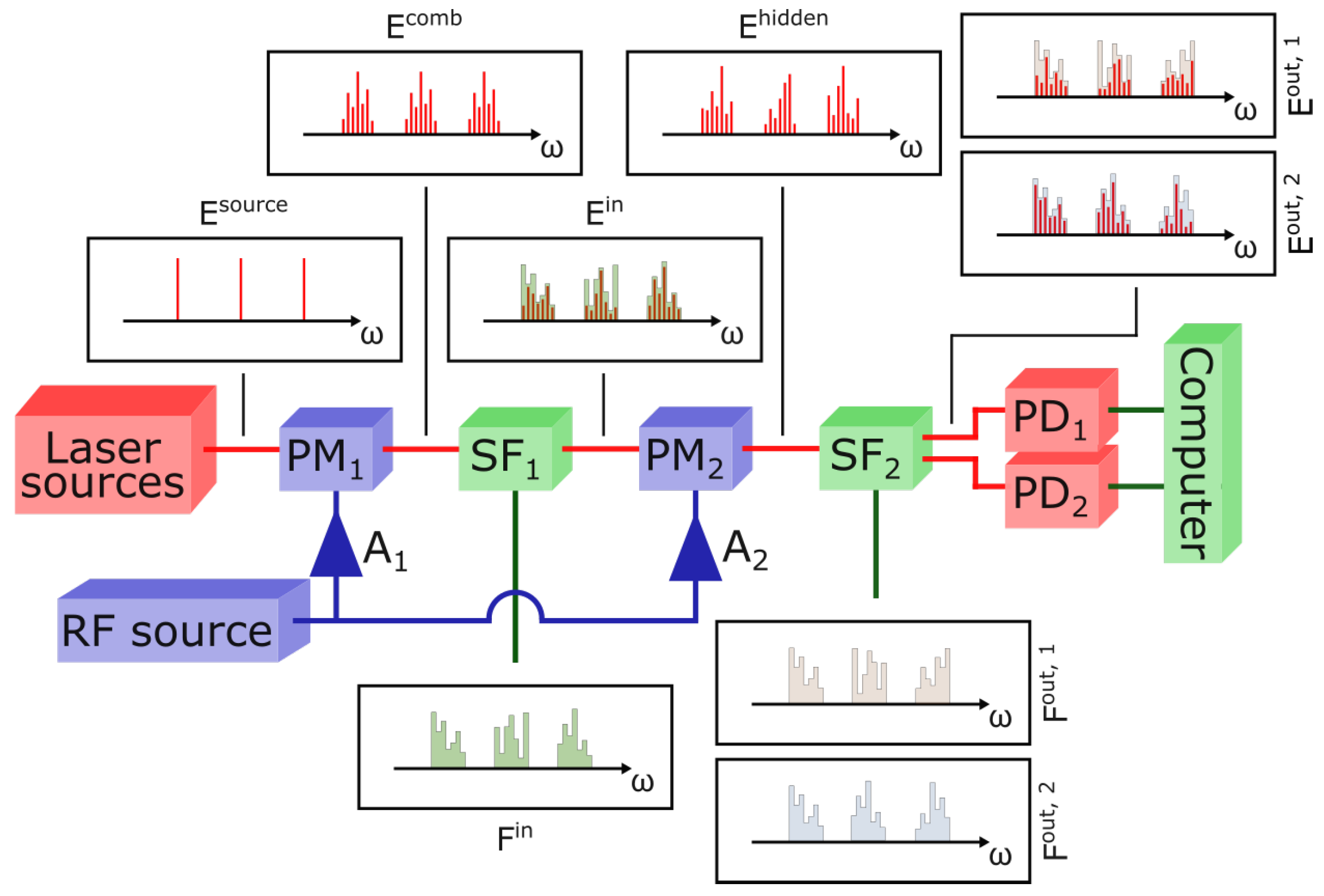
Our experimental setup is depicted in Figure 1. The light sources are three continuous wave lasers that are tunable in the C-band; we fix their wavelengths at values of nm, nm, and nm. These wavelenghts are chosen so that the frequency combs they generate do not overlap. The three sources are injected into a single optical fiber through a set of isolators and combiners; the laser output powers are set in such a way as to obtain a total optical power of approximately 9 dBm at the output of the coupling system. and are two phase modulators exploited respectively to generate the combs and mix their lines. Both modulators are driven by the same periodic Radio Frequency (RF) signal at frequency GHz. The electrical input of each phase modulator is processed by an RF amplifier ( for and for ). These two amplifiers provide two different fixed gains, hence and are driven by two different RF powers: 20 dBm and 30 dBm respectively. The effect of periodic phase modulation is more easily described by the dimensionless number , where V is the amplitude of the electrical signal and is the characteristic voltage of the phase modulator. In our setup, and . defines the spacing of comb lines and its exact value is not important as long as it does not drift significantly during the experiment. The settings are such that approximately generates a 30-line comb out of each light source (see Figure 2a). The periodic phase modulation effect is described in detail in Section 2.2, where we provide a description of the setup in terms of electric fields. For a review on electro-optic frequency comb generation, see [26]. The programmable spectral filters, and , are two Finisar Waveshapers, models 1000 and 4000, respectively. is employed to inject inputs in the network by setting the proper attenuation on each comb line, while is employed to retrieve outputs, redirecting properly filtered combs on the photodiodes and . The nominal bandwidth resolutions of the filters and are 20 GHz and 10 GHz, respectively, which should be enough to resolve a single comb line since the comb spacing is determined by . Nevertheless, we measured a slight crosstalk effect between two lines filtered by (which is, in any case, not expected to influence performances; see [19]).
2.2. Electric Field Description
Here, we describe the experiment in terms of electric fields propagating in the setup. The description is similar to what was already proposed in our previous work [19], but now accounts for the presence of multiple light sources.
Periodic phase modulation at frequency acts on a generic radiation according to the following formula:
where m is the index describing the phase modulation strength. The series expansion of the phase modulation term is known as the Jacobi–Anger expansion and shows how periodic phase modulation results in the creation of a frequency comb. represents the Bessel function of the first kind. Note that the coefficients of the expansion tend toward zero as increases. We experimentally noticed a slight asymmetry in the combs, which means that the coefficients in Equation (1) may differ from the real ones; since this effect happens in , where m is higher, we believe it is due to higher-order effects on phase modulation (see [19] for details).
We assume to have monochromatic input sources characterized by constant amplitudes with . Hence, the input radiation is as follows:
where represent the frequency of the j-th monochromatic light source. When passing through , periodic phase modulation is applied, which results in the creation of frequency combs:
where the sum over k should extend to the whole set of integer indexes, as in (1), but in practice (e.g., in simulations), it can be truncated once the coefficients become small enough. represents the phase accumulated by the radiation at frequency while travelling from the source to . The programmable spectral filter encodes input values on the comb lines, hence generating the input layer of the neural network:
where is the phase accumulated by the k-th line of the j-th comb when travelling from to , while is the attenuation that applies to the k-th comb line of the j-th comb. applies a second phase modulation, whose effect is to mix the comb line amplitudes in each comb, generating the hidden layer of the network below:
where is the phase accumulated by the p-th line of the j-th comb while travelling from to . allows for two different filter shapes to be set, redirecting the two outputs towards photodiodes and . We define as the attenuation that the spectral filter applies to the k-th line of the j-th comb before reaching , . Hence, the electric fields on the photodiodes are as follows:
where is the phase accumulated by the k-th line of the j-th comb while travelling from to the photodiodes, assuming that paths towards the two photodiodes have the same optical length. The photodiodes and provide the following intensity measurements:
where represents a time average.
3. Principle of Operation
3.1. Introduction
The working principle of the ELM scheme has been extensively described in our previous work [19]. Here, we recall the fundamental concepts and introduce the novel elements connected to the presence of multiple light sources.
In an ELM, the hidden layer is obtained by nonlinearly mixing information contained in the input layer. In our photonic implementation, the input layer is encoded in the combs by the attenuations , and the information contained therein are mixed by , generating the new set of combs that represent the hidden layer. This mixing is linear and consists in an interference of comb lines (Equation (5)). A quadratic nonlinearity is added in the readout phase (Equations (8) and (9)). The peculiarity of the proposed system consists in the way in which the information mixing works; as expressed by Equation (5), when the set of combs representing the input layer passes through , interference only happens among lines belonging to the same comb. In other words, input neurons encoded in different combs never get mixed. On the one hand, this may reduce the capability of the network to project the input data onto a higher dimensional space since the mixing of inputs is not complete. On the other hand, this allows for parallel computations that do not interfere with each other to be performed. In the following section (Section 4.2), we show that the limited dimensionality enhancement does not hinder performances when compared to an all-to-all mixing scheme.
3.2. Definitions
We denote by “single operation mode” a configuration in which the different combs are treated as parts of the same neuron layers, hence a single ELM is executed. In this case, for each data sample supplied to the network, we define by the set of input features, by the set of hidden neuron measurements, and by the target output. The network output is obtained through the multiplication of hidden neuron measurements by output weights. We define by the set of output weights and by the network output. Weights are chosen to minimize the squared error . and are row vectors composed of as many elements as lines in all the combs; depending on the dimension of the output of the specific task, and are scalar or row vectors, while is a column vector or a matrix.
We denote by “parallel operations mode” a configuration in which the different combs are treated as independent neuron layers and constitutes independent ELMs. Definitions are similar to the ones presented above, but now account for the presence of multiple ELMs. Everywhere in this paragraph, . We define by the set of input features of the j-th ELM, by the set of hidden neuron measurements of the j-th ELM, and by the target output of the j-th ELM. The output of the j-th ELM is defined by , where is the the set of optimal output weights for the j-th ELM, again obtained by minimizing the squared error .
3.3. Dataset Preprocessing
We proved in [19] that when working with a single comb, supplying the same input feature to multiple neurons may be beneficial for the network, both because it increases the mixing between input information and because it decreases the possibility that a feature gets lost by being assigned to a weak comb line. When working in single operation mode with multiple combs, redundancy is even more important since if two features are assigned to lines belonging to different combs, they do not mix in the hidden layer. Hence, when working in single operation mode, we select a random map of correspondence with repetitions, from the set of available dataset features to the set of available comb lines; instead, when working in parallel operations mode, following our previous work [19], we supply the same feature of the dataset to d consecutive comb lines, where d is optimized for each task.
Once the vector of input features is built (eventually accounting for repetitions of features, as described above), its entries are linearly converted into attenuations spanning the range of , constituting the vectors in Equation (4) supplied to the filter . In the case of the parallel operations mode, the same procedure is applied to each vector ().
The features are always encoded in the most central part of the combs, which are composed of approximately 30 lines. Central lines are preferred because they are the most powerful and can encode the inputs with the best contrast. The unused comb lines receive zero attenuation because this allows more power to take part in the mixing, which is beneficial for the system [19].
3.4. Readout
The readout procedure consists in measuring the optical intensity of each comb line, which corresponds to the values of hidden neuron states. The programmable filter is set in such a way as to implement notch filters, which select only one comb line per time. Since provides two different output ports, the readout speed is doubled by reading two different comb lines per time via the two photodiodes and . Once the vector of hidden layer measurements is recorded on the computer memory, the optimal weights are evaluated and the output is calculated on the computer. Figure 2b shows one example measurement of the hidden layer intensities recorded during the experiment.
In the case of the parallel operations mode, the readout is still executed by selecting one comb line per time through notch filters; however, now, lines of different combs represent neurons of different parallel ELMs. Thus, photodiode measurements of the j-th comb represent the hidden layer of the j-th ELM and are recorded in the vector (); for each of the ELMs executed in parallel, the computer evaluates the set of optimal weights and then calculates the output .
The output weights are estimated using the ridge regression algorithm. The optimal regularization constant is selected for each task.
In the case of classification tasks, which are the only ones tested in the present work, the ELM is required to assign a class to each set of input features. If the task provides only two possible output classes, the ELM output is a scalar value, and the prediction of the system is assumed to be one class or the other depending on whether or . If the task provides more than two output classes, the ELM output is a vector that has as many elements as the number of classes, and the prediction of the system is the class corresponding to the index of the maximal element in .
Once the optimal weights are known, they could be applied optically, setting the proper optical attenuations on in such a way that the photodiode readings represent the network output . This scheme for optical weighting has already been demonstrated in [19] but is not tested in this work.
3.5. Numerical Simulation
We developed a numerical simulation of the present scheme based on the model presented in Section 2.2 and on the operation procedures described in Section 3.3 and Section 3.4. Our simulation neglects both the effects of phases accumulated through propagation and the effects of noise.
In the following, the simulation is both proposed as a comparison for real experiments and employed to study configurations with more light sources than what is currently possible in our laboratory.
4. Results
4.1. Parallel Operations Mode
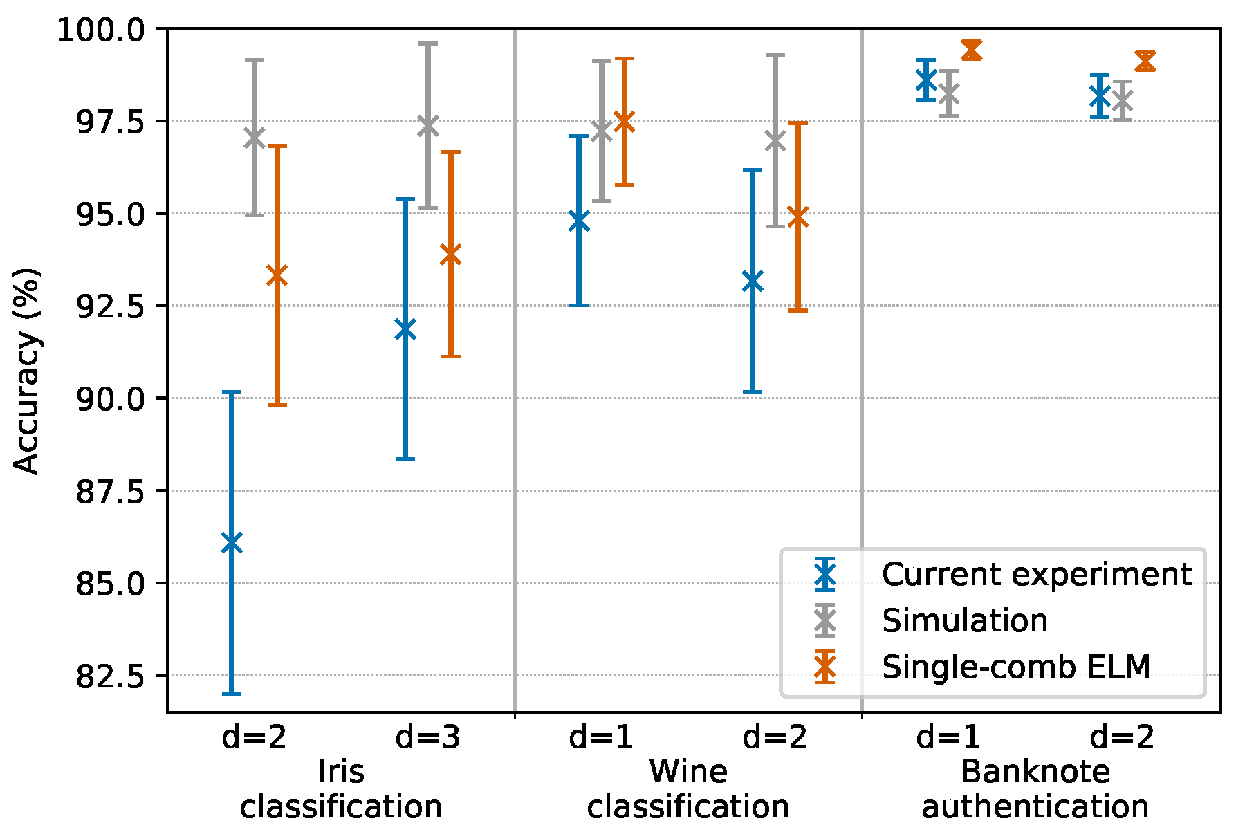
To test the ability of the system to run multiple tasks at the same time, the experiment was executed using only input light sources out of the three available ones (wavelengths and ). We tested the performances of the system on three classification tasks: iris classification [27], wine classification [28], and banknote authentication [29]. The iris classification task consists in selecting the correct class among three different ones, given a set of four different input features; the wine classification consists in selecting the correct class among three different ones, given a set of thirteen different input features; the banknote authentication task consists in selecting the correct class among two different ones, given a set of five different input features.
In Section 3.3, we discussed the convenience of encoding the same input feature to d consecutive comb lines. The best performing d values for each task were established based both on simulations and on our previous experiments [19]. For each of the tasks, we tested the two best performing d values at the same time, running two tasks in parallel, each one on a different comb. Note that in so doing, the two parallel ELMs were always running the same task type (at a given time, both were running either iris classification or wine classification or banknote authentication): this was performed as such with the sole purpose of assuring the same execution times for both ELMs; if we ran two different task types, one of the two executions would have terminated before the other since each task has a different number of database entries. This was an experimental artifice employed to test the system in a situation of full parallelism, but the ELMs are completely independent and during normal operation they are not required to finish computation at the same time. One ELM could even start a new computation while another parallel ELM is still executing a different task. Note that even when the two parallel ELMs were running the same task type, the input layers injected into the ELMs were different (since the d values were different); this implies that the hidden layers and the optimal output weights were different as well, and that the two ELMs were indeed processing different data. The results are reported in Figure 3 and are compared with a simulation and with performances obtained by our previous experiment that featured only one light source and no parallelism [19]. Each datapoint represents the average of the scores obtained by testing 100 different random repartitions of the training and testing set; the error bars represent the standard deviation of such distribution of scores.
Results clearly show that parallel operations are possible. We observed a slight decrease in accuracy when comparing the current performances with that of the previous single-comb experiment. This is likely due to the fact that the current experiment suffers from a decreased SNR, caused by power losses in the coupling between different sources, which then leads to less powerful combs.
4.2. Single Operation Mode
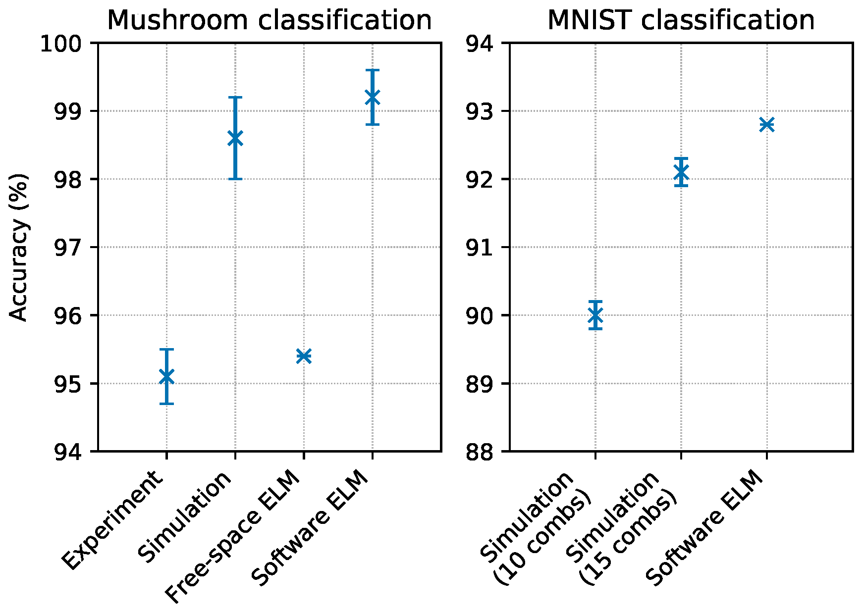
To test the capability of the system to employ all the available combs for a single computation, the experiment was executed using input light sources at wavelengths , , and . We tested the performances of the system on the mushroom classification task [30] that consists in selecting the correct class between two possible ones, given a set of 21 different input features (note that the dataset originally contained 22 features, but one of them assumes a constant value across all the entries and has thus been discarded). According to the description in Section 3.3, we encoded nine input features in the most central part of each of the three input combs. The feature order was selected at random, making sure that each feature appears at least once, and that six features appears twice, in two different combs. Results are reported in Figure 4. The accuracy of the classification is , where the score is the average measured across 100 different random repartitions of the training and the testing set, and the error is the standard deviation of such distribution of scores. A software ELM composed of 90 hidden neurons with quadratic nonlinearity reached an accuracy of , where the score was evaluated as described above. A simulation of this multi-comb scheme reached an accuracy of , where the score was the average measured across 100 possible redistributions of the 21 features in the three combs, and the error was the standard deviation of such distribution of scores. A photonic ELM exploiting free-space propagation in a scattering medium [8] scored an accuracy of on this same task.
To better investigate this single operation scheme, we conducted a test via numerical simulation on the MNIST handwritten digit classification task [31], which could not be implemented on a single-comb system since it required too many neurons. The only preprocessing of the dataset consisted in a resampling of the input images: we submitted to the network images composed of pixels, corresponding to 289 input features. We simulated a system similar to the current one, with the only difference that it contained light sources, each one generating a comb, resulting in approximately 300 input neurons and 300 hidden ones. The simulation reached an accuracy of . When we simulated the same system with , which corresponds to 450 input neurons and 450 hidden ones, the accuracy increased to . Note that our present system with light sources has comb lines, which is not enough to encode the 289 input features; however, the scenarios with or light sources are potentially realisable experimentally (see Section 5). A software ELM reported in [32] was tested on the same classification task, with no image resampling. When executed with 784 input neurons, 784 hidden neurons, and a tanh nonlinearity, this ELM reached an accuracy of (the accuracy could be increased up to approximately , increasing the number of hidden neurons by 20 times).
These results clearly show that merging multiple independent combs in a single ELM is a viable way of tackling tasks that require a high number of neurons. In particular, the results of the NMIST numerical simulation show how the way in which the hidden layer is generated constitutes a good mixing since the performances are comparable with that of the software ELM, despite the fact that the latter is composed of more neurons.
5. Conclusions
In this work we explored the parallelization capabilities of a photonic ELM based on frequency multiplexing, which had been hypothesized in our previous work [19]. We proved that propagating multiple light sources in the same setup allows both for an increase in the number of available neurons and for the execution of multiple non-interacting tasks. This parallelized scheme is expected to remain compatible with the optical weightning scheme proposed in [19], even if no experiment has been run in this sense yet.
When compared with an identical experiment run with a single light source, the current scheme displayed a slight decrease in performance. We expected this effect to be completely avoidable by increasing the SNR of data encoded in the combs, which can be obtained by increasing the light source power, by introducing optical amplification, or by reducing the losses at the laser source combiners.
Our ELM performed similarly to a photonic one based on free-space propagation [8] when both were tested on the same task (mushroom classification). Numerical simulations also suggest that our scheme would perform similarly to a software ELM on tasks requiring hundreds of neurons such as MNIST digit classification.
We tested the system with a maximum of sources, but this number could be significantly increased. The C-band spans THz and can hence accommodate approximately 300 neurons at the current spacing of GHz, which means approximately 10 different combs similar to the ones employed in the current experiment. Moreover, could be decreased, which would lead to a more dense frequency multiplexing, provided that the employed spectral filters have enough resolution.
We also note that the broadness of the comb itself could be increased or decreased, modifying the RF power driving and (hence, acting on the values and ). In principle, a lower value would generate smaller combs, allowing for even more operations in parallel to be executed at the expense of the number of neurons available for each operation.
The main drawback of the current scheme is the information processing speed, limited by the programmable spectral filters whose maximum update rate is . Nevertheless, this speed can, in principle, be increased considerably. For instance, an integrated photonic version of this scheme may rely on a programmable spectral filter realized by a combination of WDM filters and electroptical absorption modulators, which should theoretically allow GHz rates to be reached.
The present work further demonstrates the potential of photonic information processing in the frequency domain, particularly for ELMs.
Author Contributions
Conceptualization, A.L. and S.M.; data curation, A.L.; funding acquisition, S.M.; investigation, A.L.; methodology, A.L. and S.M.; project administration, S.M.; software, A.L.; supervision, S.M.; visualization, A.L.; writing—original draft, A.L; writing—review and editing, S.M. All authors have read and agreed to the published version of the manuscript.
Funding
The authors acknowledge financial support from the European Union through the Marie Skłodowska-Curie Innovative Training Networks action, POST-DIGITAL project number 860830, and from the Fonds de la Recherche Scientifique (FRS-FNRS).
Institutional Review Board Statement
Not applicable.
Informed Consent Statement
Not applicable.
Data Availability Statement
Data underlying the results presented in this paper are not publicly available at this time but may be obtained from the authors upon reasonable request.
Acknowledgments
The authors thank Ghent University-IMEC for the loaning of a Waveshaper.
Conflicts of Interest
The authors declare no conflict of interest.
References
- Scardapane, S.; Wang, D. Randomness in Neural Networks: An Overview. Wiley Interdiscip. Rev. Data Min. Knowl. Discov. 2017, 7, e1200. [Google Scholar] [CrossRef]
- Huang, G.B.; Zhu, Q.Y.; Siew, C.K. Extreme learning machine: A new learning scheme of feedforward neural networks. In Proceedings of the IEEE International Joint Conference on Neural Networks, Budapest, Hungary, 25–29 July 2004; pp. 985–990. [Google Scholar] [CrossRef]
- Huang, G.B.; Zhu, Q.Y.; Siew, C.K. Extreme learning machine: Theory and applications. Neurocomputing 2006, 70, 489–501. [Google Scholar] [CrossRef]
- Huang, G.B. What are extreme learning machines? Filling the gap between Frank Rosenblatt’s dream and John von Neumann’s puzzle. Cognit. Comput. 2015, 7, 263–278. [Google Scholar] [CrossRef]
- Gonon, L.; Grigoryeva, L.; Ortega, J.P. Approximation bounds for random neural networks and reservoir systems. arXiv 2002, arXiv:2002.05933v2. [Google Scholar]
- Xu, R.; Lv, P.; Xu, F.; Shi, Y. A survey of approaches for implementing optical neural networks. Opt. Laser Technol. 2021, 136, 106787. [Google Scholar] [CrossRef]
- Saade, A.; Caltagirone, F.; Carron, I.; Daudet, L.; Drémeau, A.; Gigan, S.; Krzakala, F. Random projections through multiple optical scattering: Approximating Kernels at the speed of light. In Proceedings of the IEEE International Conference on Acoustics, Speech and Signal Processing, Shanghai, China, 20–25 March 2016; pp. 6215–6219. [Google Scholar] [CrossRef] [Green Version]
- Pierangeli, D.; Marcucci, G.; Conti, C. Photonic extreme learning machine by free-space optical propagation. Photonics Res. 2021, 9, 1446–1454. [Google Scholar] [CrossRef]
- Tegin, U.; Yıldırım, M.; Oguz, I.; Moser, C.; Psaltis, D. Scalable Optical Learning Operator. arXiv 2012, arXiv:2012.12404. [Google Scholar]
- Ortín, S.; Soriano, M.C.; Pesquera, L.; Brunner, D.; San-Martín, D.; Fischer, I.; Mirasso, C.; Gutiérrez, J. A unified framework for reservoir computing and extreme learning machines based on a single time-delayed neuron. Sci. Rep. 2015, 5, 14945. [Google Scholar] [CrossRef] [Green Version]
- Appeltant, L.; Soriano, M.C.; Sande, G.V.D.; Danckaert, J.; Massar, S.; Dambre, J.; Schrauwen, B.; Mirasso, C.R.; Fischer, I. Information processing using a single dynamical node as complex system. Nat. Commun. 2011, 2, 468. [Google Scholar] [CrossRef] [Green Version]
- Paquot, Y.; Duport, F.; Smerieri, A.; Dambre, J.; Schrauwen, B.; Haelterman, M.; Massar, S. Optoelectronic reservoir computing. Sci. Rep. 2012, 2, 287. [Google Scholar] [CrossRef]
- Larger, L.; Soriano, M.C.; Brunner, D.; Appeltant, L.; Gutierrez, J.M.; Pesquera, L.; Mirasso, C.R.; Fischer, I. Photonic information processing beyond Turing: An optoelectronic implementation of reservoir computing. Opt. Express. 2012, 20, 3241–3249. [Google Scholar] [CrossRef]
- Rodan, A.; Tiňo, P. Simple Deterministically Constructed Recurrent Neural Networks. In Intelligent Data Engineering and Automated Learning—IDEAL 2010; Fyfe, C., Tino, P., Charles, D., Garcia-Osorio, C., Yin, H., Eds.; Springer: Berlin/Heidelberg, Germany, 2010; pp. 267–274. [Google Scholar]
- Bueno, J.; Maktoobi, S.; Froehly, L.; Fischer, I.; Jacquot, M.; Larger, L.; Brunner, D. Reinforcement learning in a large-scale photonic recurrent neural network. Optica 2018, 5, 756–760. [Google Scholar] [CrossRef] [Green Version]
- Antonik, P.; Marsal, N.; Brunner, D.; Rontani, D. Human action recognition with a large-scale brain-inspired photonic computer. Nat. Mach. Intell. 2019, 1, 530–537. [Google Scholar] [CrossRef] [Green Version]
- Vandoorne, K.; Mechet, P.; Van Vaerenbergh, T.; Fiers, M.; Morthier, G.; Verstraeten, D.; Schrauwen, B.; Dambre, J.; Bienstman, P. Experimental demonstration of reservoir computing on a silicon photonics chip. Nat. Commun. 2014, 5, 3541. [Google Scholar] [CrossRef] [Green Version]
- Butschek, L.; Akrout, A.; Dimitriadou, E.; Haelterman, M.; Massar, S. Parallel photonic reservoir computing based on frequency multiplexing of neurons. arXiv 2008, arXiv:2008.11247. [Google Scholar]
- Lupo, A.; Butschek, L.; Massar, S. Photonic extreme learning machine based on frequency multiplexing. Opt. Express 2021, 29, 28257–28276. [Google Scholar] [CrossRef] [PubMed]
- Xu, X.; Tan, M.; Corcoran, B.; Wu, J.; Nguyen, T.G.; Boes, A.; Chu, S.T.; Little, B.E.; Morandotti, R.; Mitchell, A.; et al. Photonic Perceptron Based on a Kerr Microcomb for High-Speed, Scalable, Optical Neural Networks. Laser Photonics Rev. 2020, 14, 2000070. [Google Scholar] [CrossRef]
- Xu, X.; Tan, M.; Corcoran, B.; Wu, J.; Boes, A.; Nguyen, T.G.; Chu, S.T.; Little, B.E.; Hicks, D.G.; Morandotti, R.; et al. 11 TOPS photonic convolutional accelerator for optical neural networks. Nature 2021, 589, 44–51. [Google Scholar] [CrossRef] [PubMed]
- Feldmann, J.; Youngblood, N.; Karpov, M.; Gehring, H.; Li, X.; Stappers, M.; Le Gallo, M.; Fu, X.; Lukashchuk, A.; Raja, A.S.; et al. Parallel convolutional processing using an integrated photonic tensor core. Nature 2021, 589, 52–58. [Google Scholar] [CrossRef] [PubMed]
- Duan, M.; Li, K.; Liao, X.; Li, K. A Parallel Multiclassification Algorithm for Big Data Using an Extreme Learning Machine. IEEE Trans. Neural Netw. Learn. Syst. 2018, 29, 2337–2351. [Google Scholar] [CrossRef]
- Brunner, D.; Soriano, M.C.; Mirasso, C.R.; Fischer, I. Parallel photonic information processing at gigabyte per second data rates using transient states. Nat. Commun. 2013, 4, 1364. [Google Scholar] [CrossRef] [PubMed] [Green Version]
- Duport, F.; Smerieri, A.; Akrout, A.; Haelterman, M.; Massar, S. Virtualization of a Photonic Reservoir Computer. J. Light. Technol. 2016, 34, 2085–2091. [Google Scholar] [CrossRef]
- Parriaux, A.; Hammani, K.; Millot, G. Electro-optic frequency combs. Adv. Opt. Photonics 2020, 12, 223. [Google Scholar] [CrossRef]
- Fisher, R. Iris Data Set. Available online: http://archive.ics.uci.edu/ml/datasets/iris (accessed on 15 November 2021).
- Forina, M. Wine Data Set. Available online: https://archive.ics.uci.edu/ml/datasets/wine (accessed on 15 November 2021).
- Lohweg, V. Banknote Authentication Data Set. Available online: https://archive.ics.uci.edu/ml/datasets/banknote+authentication (accessed on 15 November 2021).
- Lincoff, G.H. Mushroom Data Set. Available online: https://archive.ics.uci.edu/ml/datasets/mushroom (accessed on 15 November 2021).
- LeCun, Y.; Cortes, C.; Burges, C.J.C. MNIST Database of Handwritten Digits. Available online: http://yann.lecun.com/exdb/mnist/ (accessed on 15 November 2021).
- de Chazal, P.; Tapson, J.; van Schaik, A. A comparison of extreme learning machines and back-propagation trained feed-forward networks processing the mnist database. In Proceedings of the 2015 IEEE International Conference on Acoustics, Speech and Signal Processing (ICASSP), South Brisbane, Australia, 19–24 April 2015. [Google Scholar] [CrossRef]
Figure 1.
Scheme of the experimental setup. Red lines represent optical connections, green lines represent data connection to and from the computer, and blue lines represent RF connections. and represent two RF amplifiers. The first Phase Modulator, , generates a frequency comb out of each line in the spectrum of the light source, . The first programmable Spectral Filter, , encodes input features in these combs, thus generating the input layer (or the set of input layers, in the case of parallel operations). The filter shape loaded onto , , is calculated according to the features to be encoded. The second Phase Modulator, , mixes the components of , thus generating the hidden layer (or the set of hidden layers, in the case of parallel operations). The second programmable Spectral Filter, , is employed for the readout and can apply two different filter shapes ( and ) to its two outputs, generating and . The photodiodes and measure the total intensities in and , respectively. A computer drives the programmable filters (connections not shown) and records the photodiode measurements. To measure the hidden layer, the combs are scanned one line at a time by programming with notch filters. The output can then be computed offline as a linear combination of the intensities of the spectral lines. The figure shows a possible implementation of optical weighting, as demonstrated in [19], where applies attenuations proportional to the desired weights.

Figure 2.
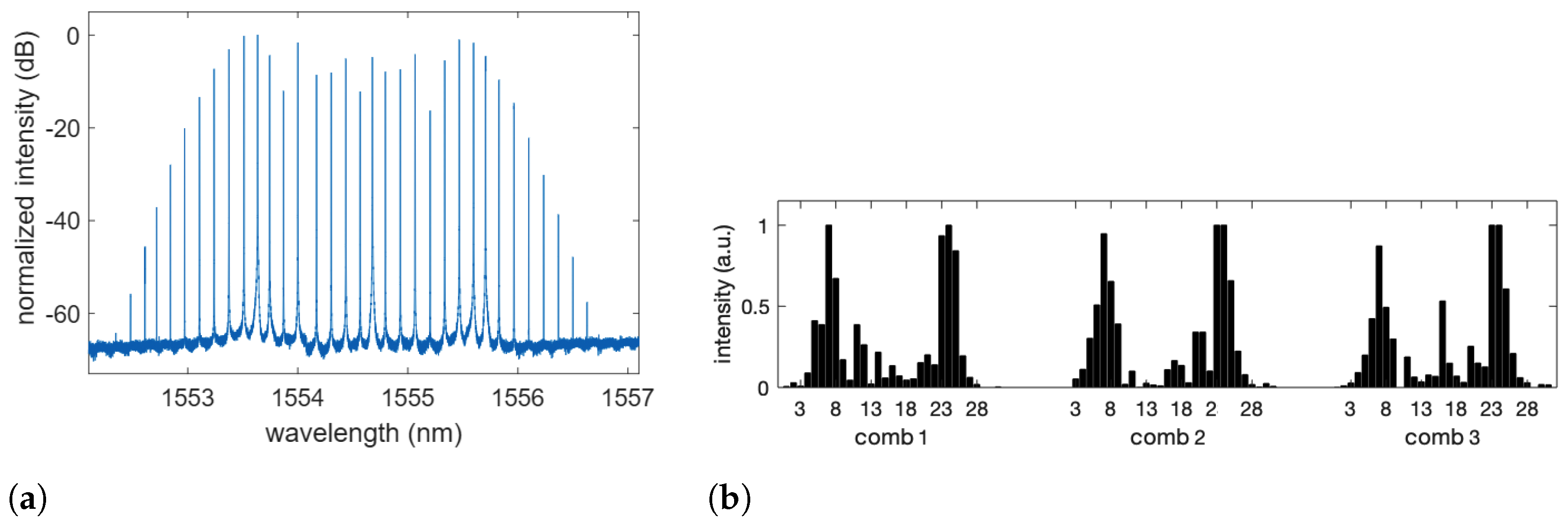
(a) Example of spectral comb recorded at the output of . For this measurement, a single CW laser source was employed at the wavelength nm. RF modulation was GHz, corresponding to a difference in wavelength of approximately 137 pm. The resulting comb has approximately 30 usable lines, which correspond to a bandwidth of approximately 4 nm. (b) Example of comb line intensities of the hidden layer, as measured by and . The task being solved is the mushroom classification in the single operation mode. Three combs are used at the same time, each one comprising 31 comb lines numbered from 1 to 31.
Figure 2.
(a) Example of spectral comb recorded at the output of . For this measurement, a single CW laser source was employed at the wavelength nm. RF modulation was GHz, corresponding to a difference in wavelength of approximately 137 pm. The resulting comb has approximately 30 usable lines, which correspond to a bandwidth of approximately 4 nm. (b) Example of comb line intensities of the hidden layer, as measured by and . The task being solved is the mushroom classification in the single operation mode. Three combs are used at the same time, each one comprising 31 comb lines numbered from 1 to 31.

Figure 3.
Results of parallel operations mode tests. d indicates the number of consecutive comb lines on which each feature is encoded. The same task types with different d values are executed in parallel on two different combs. Each result is compared with the numerical simulation and previous experiments of a single-comb ELM [19]. Error bars represent the standard deviation of the score over 100 random repartitions of training and testing data (more information in Section 4.1).

Figure 4.
Results of single operation mode tests. The left panel contains results from the mushroom classification task. We report experimental results compared with the numerical simulation of our system, the score obtained by another photonic ELM reported in [8], and a software ELM with a number of neurons comparable to our experiment. The right panel contains results from the MNIST classification task. We report the results obtained by a numerical simulation featuring 10 combs (∼300 neurons), a numerical simulation featuring 15 combs (∼450 neurons), and a software ELM reported in [32] (∼800 neurons). When present, error bars represent the standard deviation of the score over 100 random repartitions of training and testing data (more information in Section 4.2).

Publisher’s Note: MDPI stays neutral with regard to jurisdictional claims in published maps and institutional affiliations. |
© 2021 by the authors. Licensee MDPI, Basel, Switzerland. This article is an open access article distributed under the terms and conditions of the Creative Commons Attribution (CC BY) license (https://creativecommons.org/licenses/by/4.0/).
Share and Cite
MDPI and ACS Style
Lupo, A.; Massar, S. Parallel Extreme Learning Machines Based on Frequency Multiplexing. Appl. Sci. 2022, 12, 214. https://doi.org/10.3390/app12010214
AMA Style
Lupo A, Massar S. Parallel Extreme Learning Machines Based on Frequency Multiplexing. Applied Sciences. 2022; 12(1):214. https://doi.org/10.3390/app12010214
Chicago/Turabian StyleLupo, Alessandro, and Serge Massar. 2022. "Parallel Extreme Learning Machines Based on Frequency Multiplexing" Applied Sciences 12, no. 1: 214. https://doi.org/10.3390/app12010214
Note that from the first issue of 2016, this journal uses article numbers instead of page numbers. See further details here.