Advancing best practices for assessing trends of ocean acidification time series

1 Introduction

Ocean acidification is a major concern of many local and global-scale decision makers due to potential impacts to marine ecosystem health and food security (Gattuso et al., 2015; Doney et al., 2020). While primarily driven by the global increase in carbon dioxide (CO₂) emissions, ocean acidification impacts (e.g., reduced pH and lower availability of carbonate ions to calcifying organisms like shellfish and corals) can progress differently in different regions. These impacts can be particularly variable in coastal waters where additional drivers, including both human-caused and natural processes such as changing circulation patterns, nutrient runoff, and biological productivity, vary greatly over both time and space (Mongin et al., 2016; Chan et al., 2017; Cai et al., 2021).

Scientific and societal demand for ocean acidification status and trend data is increasing. For example, annual reporting on global seawater pH observations is called for under United Nations Sustainable Development Goal (UN SDG) 14. Ocean acidification is also a headline climate indicator for the World Meteorological Organization (WMO). In the United States, multiple states have included ocean acidification monitoring as a priority in their environmental and water quality assessment needs (Weisberg et al., 2016). Due to strong cultural, economic, and recreational dependencies on marine organisms vulnerable to ocean acidification, the states of Washington, Oregon, California, and Hawaii have developed action plans to further assess status, understand drivers, and evaluate adaptation strategies (Adelsman and Binder, 2012; Chan et al., 2016; State of Hawaii, 2021). Canada’s Oceans Now review of the three oceans surrounding Canada is regularly assessing the status of ocean chemistry and potential biological impacts of acidified waters (Canada’s Oceans Now 2020). Ocean acidification has been identified as one of five top climate change risks by British Columbia’s preliminary strategic climate risk assessment (Ministry of Environment and Climate Change Strategy, 2019). Ocean acidity is also a marine environmental indicator for New Zealand, with data from open ocean and coastal monitoring sites reported and analyzed every two years. Communicating how ocean acidification is progressing in one region compared to another within these types of international and national assessments requires consistent protocols for analyzing and reporting trends.

If ocean acidification trend and status assessments are to be comparable, observational data must also be collected using standardized measurement protocols with common reference materials. The global ocean acidification community has leveraged and expanded standard operating procedures (SOPs) for making ocean carbonate chemistry measurements (Dickson et al., 2007; Riebesell et al., 2011). These SOPs were most recently modified for low-cost analysis of ocean acidification measurements and are available in several languages at www.goa-on.org/resources/kits.php. Uniform observational data quality and accessibility standards have also matured through several international community efforts, including the Global Ocean Acidification Observing Network (GOA-ON; GOA-ON, 2019), the Surface Ocean CO₂ Atlas (SOCAT; Bakker et al., 2016), and the Global Ocean Data Analysis Project (GLODAP; Lauvset et al., 2021).

The data sets generated by these standardized measurement and data quality protocols can be valuable tools for characterizing how the ocean is changing over time. However, there are currently no standardized approaches for assessing and reporting trends from ocean carbon time-series data sets. Standardization of trend analysis is necessary to enable comparisons across ocean and coastal systems globally, create accurate records of change that stand the test of time, and communicate scientific results clearly and consistently to policy makers and the public.

Here we build off initial work described in Sutton and Newton (2020) to develop best practices for uniform analyses and presentation of multi-decadal changes in ocean acidification time series, including open-source software to support these analyses. These techniques could also extend to analysis of other ocean biogeochemical parameters, particularly when the goal is to understand the processes driving change in interconnected biogeochemical cycles, such as the carbon and nitrogen cycles. These best practices are a first attempt at combining several common approaches into a standard methodology for varied ocean time-series data. However, these best practices must evolve along with the evolving state of the data sets and the techniques used in trend analysis, particularly related to different linear regression models (e.g., Franco et al., 2021) and gap-filling techniques (e.g., Vance et al., 2022) able to create continuous time series that can be analyzed using statistical-based signal processing approaches. We recommend these best practices be revisited and updated by a formalized community of practice on a regular basis.

2 Lessons learned from established best practices

We draw upon decades of work by the atmospheric community in uniform analysis and reporting of CO₂ trends (Tsutsumi et al., 2009). However, there are key distinctions between the ocean and atmospheric carbon communities related to the analysis and reporting of trends. First, atmospheric measurements of CO₂ are more abundant. There are hundreds of atmospheric CO₂ fixed time-series stations compared to a couple dozen established ocean acidification and carbonate system time-series sites, primarily in the open ocean. The ocean carbonate chemistry time-series sites providing 10 years or more of publicly-available data are shown in Figure 1. This figure is likely incomplete, given there is currently no fully comprehensive, centralized location or portal for accessing metadata or data related to all ocean carbon time series. These locations were identified by assessing length of publicly-available ocean carbon time series and data collection frequency through GOA-ON, OceanSITES, and the EarthCube Research Coordination Network for Marine Ecological Time Series.

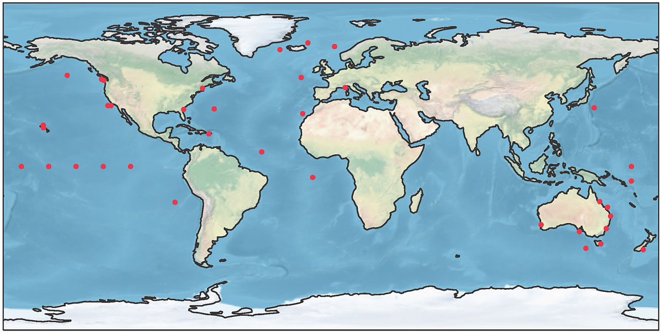
Figure 1 Locations of fixed time series with active programs collecting ocean carbonate chemistry data on ships or moored buoys at sub-seasonal timescales and providing access to ≥10 years of publicly-available data.

Most of the ocean acidification time-series sites located in highly-variable coastal regions have only been established in the last ten years and have experienced recent data gaps due to the impact of COVID-19 on ocean observing (Boyer et al., in review). Due to the high signal to noise ratio, such data sets require frequent sampling and longer observational records to detect a long-term signal over natural variability (Carter et al., 2019; Sutton et al., 2019; Turk et al., 2019). Both the atmospheric and ocean carbonate chemistry observing communities have established some “baseline” observatories that have been used to monitor trends, such as the Mauna Loa Atmospheric Baseline Observatory, Hawaii Ocean Time-series (HOT) project, and Bermuda Atlantic Time-series Study (BATS), in locations away from continents and coastal areas where atmospheric CO₂ and ocean acidification variability tend to be stronger.

Additional distinctions between the ocean and atmosphere are that the marine boundary layer of the atmosphere is much more well-mixed than the surface ocean, and atmospheric CO₂ has a smaller seasonal signal, especially compared to coastal ocean carbonate chemistry. Where there are data gaps in the atmospheric CO₂ record, those gaps can be statistically-interpolated based on well-defined CO₂ variations over both space and time (Masarie and Tans, 1995). However, these same approaches can introduce large errors when applied to ocean carbonate chemistry time series that are discontinuous, sparse, and have uncharacterized variability (Vance et al., 2022).

Key concepts included in best practices for atmospheric CO₂ trend analysis include selecting fixed time-series data sets that follow standardized methodologies and meet community-defined and uniform data quality, determining and removing the periodic signal(s) in the time series, and applying uniform procedures for calculating and reporting trends and associated uncertainties. Other important processes we draw from the atmospheric community’s experience are publishing transparent protocols, as is the goal here, and meeting regularly to intercompare and reassess methods.

3 Best practices for assessing trends of ocean acidification time series

Characterizing ocean acidification time-series trends requires a sequence of approaches, broadly described as:

1. assess data gaps in the time series;

2. remove periodic signals (i.e., normally occurring variations due to predictable cycles) from the time series;

3. assess a linear fit to the data with the periodic signal(s) removed;

4. estimate whether a statistically-significant trend can be detected from the time series;

5. consider uncertainty in the measurements and reported trends; and

6. present trend analysis results in the context of natural variability and uncertainty.

Each of these steps are described in detail in the following subsections. Many of the procedures outlined in these steps have been utilized in past studies to assess trends and variability in ocean carbonate chemistry observations (Bates, 2001; Takahashi et al., 2009; Bates et al., 2014; Sutton et al., 2019). However, this is the first time they have been packaged together and expanded into a best practice for assessing and reporting ocean acidification trends. This does not preclude scientists from continuing to develop and evaluate other time-series analysis approaches in their research, as that is an important research need. Rather, the goal here is to establish a readily-accessible protocol that can be implemented and applied by GOA-ON, the Ocean Acidification Research for Sustainability (OARS) program, UN SDG, WMO, and individual researchers when the intention is to compare trends across different regions on a variety of data sets generated by different research groups. In addition to reporting on trends that result from these best practices, researchers are encouraged to report on other gap-filling and time-series analysis techniques that best suit their data. This additional research and reporting will inform future updates to the best practices presented here.

Wherever possible, the trend analysis should be done on ocean carbonate chemistry parameters that have been measured using established SOPs (Dickson et al., 2007), including: dissolved inorganic carbon (DIC), total alkalinity (TA), the partial pressure or fugacity of CO₂ (pCO₂ or fCO₂), or pH (at measurement temperature and in total hydrogen ion scale). Temperature and salinity measurements also need to be calibrated and of high quality. If measured or calculated pH is used in the trend analysis, we recommend presenting results in terms of both hydrogen ion concentration, [H⁺], and pH as recommended by Fassbender et al. (2020) because pH is on the logarithmic scale, and regional differences in the mean state of pH influence the magnitude of change, hindering comparisons of pH change across different regions. While these best practices assess linear trends, seawater pH will have a non-linear trend over long periods of time, and atmospheric CO₂ growth since preindustrial times has been roughly exponential. As ocean carbonate chemistry time series increase in data density and duration, it may be beneficial to report decadal averages of trends, which is a best practice of the atmospheric CO₂ community.

When presenting results of calculated parameters, uniform use of constants should be applied to generate comparable results across different time series. As of the time of publication, the community’s current best practices (Orr et al., 2018) are to use the carbonic acid dissociation constants of Lueker et al. (2000), sulfate dissociation constants of Dickson (1990), and borate-to-salinity ratio of Lee et al. (2010) to calculate the carbon system. Future updates to these best practices should assess how these protocols need to be revised to better accommodate low-salinity environments, such as estuaries, at a range of temperatures (Schockman and Byrne, 2021). For example, the carbonic acid dissociation constants of Waters et al. (2014) may be more appropriate for low-salinity coastal waters (salinity< 19; Orr et al., 2018).

Since ocean carbonate chemistry observations are often collected along with other physical and biogeochemical parameters, such as dissolved oxygen and inorganic nutrients, extending the analysis to include these parameters can provide insight into the factors contributing to inter-annual or multi-decadal change. If seawater temperature, evaporation, or precipitation changes over time may be driving carbonate system change in the time series, the temperature effect can be removed (e.g., for pCO₂ or fCO₂ as described by Takahashi et al., 2002) or salinity-normalized parameters (e.g., salinity-normalized DIC as applied to time series by Bates et al., 2014) could also be included in the trend analysis. For example, if a region is experiencing increased pCO₂ and seawater temperature, different ocean carbonate parameters like pCO₂ (impacted by both increasing CO₂ and temperature) and DIC (impacted by increasing CO₂ but not temperature) will have different relative trends. While there is some potential to introduce variability in salinity-normalized DIC across different time series by using mean salinity in the normalization rather than prescribing a salinity of 35, using the time series mean will accommodate the calculation of salinity-normalized DIC trends in low-salinity environments. However, in regions of significant and variable river inputs or sea ice melt, the simple salinity normalization (assuming DIC and TA are only concentrated by evaporation or diluted by precipitation) will introduce river or sea ice endmember-induced artifacts (Jiang et al., 2008; Bates et al., 2009), and a more appropriate normalization to count the effect of river endmembers should be considered (Friis et al., 2003).

Finally, we make assumptions about the underlying data in the approach described in the following sections. We assume that data quality control is performed prior to determining the trend. No time series should be used without assessing data quality and, when necessary, making adjustments (e.g., in the case of a change in methodology) to create a homogenous time series. All the time-series data should be subject to the same biases and have equal precision, and if gaps in the data exist, they should not impact the calculations of climatological monthly or annual means. We also assume that monthly means are normally distributed and temporally autocorrelated, as is common in environmental time series. If a seasonal signal exists, that signal and the climatological mean should be able to be characterized using the data set. This is most straightforward for fixed time series where data collection frequency is at monthly or sub-monthly time scales. However, it may be possible to constrain climatological monthly means with less frequent observations if the time series is long enough and all months are represented in the data set.

3.1 Assess data gaps

In this approach we assume all observations in a time series are subject to the same biases and have equal precision. Any change in the data should only reflect a change in real world conditions, not changes in the measurement methodologies or the location where the time-series data are collected. Although statistical approaches exist that allow trend assessments on time series with dissimilar observation types, more research is needed to determine whether these approaches are applicable to ocean biogeochemical data. For the best practices proposed here, the user should assess and correct for changes in methodology or site location prior to determining the time-series trend. A t-test or standard normal homogeneity test can be used to determine whether a change of method or location has a significant impact on the data (WMO, 2020). Before adjusting the time series, the user should consider whether the changes in methodology or site location will impact the trend analysis significantly, and if so, whether it is better to use a shorter time series with uniform methodologies or a longer time series that has been adjusted.

The first step in these best practices is to assess whether data gaps may introduce a bias in the climatology used to remove the periodic signal (Section 3.2). Excessive or insufficient data density can also be an issue for time series, particularly when combining different observation types (e.g., five years of monthly samples that are supplemented by five subsequent years of nearly-continuous sensor readings). Regularizing data in time can be accomplished by upsampling poorly-resolved periods (i.e., creating higher-resolution data) using interpolation or downsampling portions of the record that are measured at abnormally high frequency (i.e., creating lower-resolution data) using, for example, bin averaging. Upsampling is only appropriate when you are confident that the interpolated data series captures all meaningful variations, and in this application, it is typically better to downsample the highly-resolved portions of the record.

Data gaps do not always have a significant impact on trend analysis, but this needs to be assessed for each time series. Ocean carbonate chemistry data sets typically contain gaps, and as a result, there is a compromise between having homogenous, complete data sets and having enough ocean acidification time-series data available to determine trends within an acceptable level of uncertainty. Given one aim of these best practices is to support trend comparisons across different regions on data from different research groups, any gap-filling technique must be amenable to a variety of data sets. In a recent assessment of different statistical and empirical methods for filling gaps in ocean carbon time series, Vance et al. (2022) found that an empirical multivariate linear regression (MLR) model provided the most robust approach across different open ocean and coastal regions with several variations in the timing and duration of data gaps. In this MLR approach, gaps in DIC observations were filled with DIC estimated from satellite-based chlorophyll, sea surface temperature, and salinity with an uncertainty of about 9 µmol kg^-1 for open ocean time-series sites and 20 µmol kg^-1 at coastal sites. However, it is unlikely that one type of MLR approach using the same satellite-based data inputs will be able to reproduce ocean carbonate chemistry at all ocean acidification time-series locations, complicating direct trend comparisons between open ocean and coastal sites (Figure 1). Further assessment of whether any empirical or statistical techniques could be used to fill data gaps without introducing bias to the resulting trend is an area where additional focus is needed.

In the trend analysis methods presented here, gaps in the original time series are not filled. Rather, the assessment of data gaps is primarily focused on whether monthly climatologies calculated from that time series represent actual ocean carbonate chemistry conditions and can serve as a benchmark for removing seasonal variability from the data set. In this approach, gaps can introduce errors to the trend analysis if there is insufficient data density within a certain portion of the climatology. For example, if the only observations within a certain month were collected during anomalous conditions, the estimated monthly mean is not likely representative of actual monthly mean conditions (e.g., Figure 2A). In this scenario, users may choose to modify sampling plans to collect more observations to better constrain the seasonal signal or to proceed with the understanding that insufficient data density may add additional uncertainty to the analysis. In another scenario, if the time series is in a region where data are only collected during certain seasons (e.g., April through October as in Figure 2B), the results of the time-series analysis would only apply to the trend during those seasons and should be reported as such. These are decisions the user must make based on their knowledge of the data set and region they are studying.

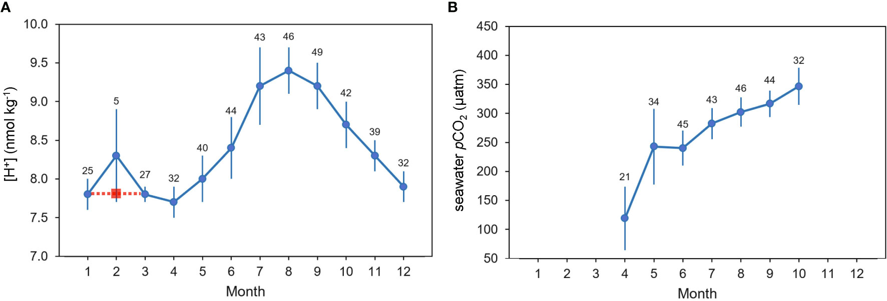
Figure 2 Examples illustrating climatological monthly means (blue circles with standard deviation as error bars): (A) an example of a continuous time series lacking a sufficient number of February observations of [H⁺], (adapted from Figure 2 in Takahashi et al., 2009) and (B) an example of a seawater pCO₂ (µatm) time series with repeat measurements only collected during the months of April through October. Sample sizes are listed above each monthly mean. The red square illustrates a February mean interpolated between surrounding months with sufficient data density compared to a mean generated from potentially insufficient data density.

3.2 Remove periodic signal(s)

Characterizing and removing the periodic signal(s) prior to estimating trends reduces variability (or noise) and autocorrelation in environmental data sets, thereby reducing uncertainty in the resulting trend. Many statistical signal processing approaches exist that are capable of removing the periodic signal(s) from continuous data sets with regular sampling intervals (e.g., as for atmospheric CO₂ described in Tsutsumi et al., 2009). However, we use an alternative approach for discontinuous data sets common in the ocean carbon community (Bates, 2001; Takahashi et al., 2009; Bates et al., 2014). These approaches only work if the time series is longer than several multiples of the cycle itself because they rely on using multiple observations of the cycle to characterize its mean impact on the signal.

Prior to characterizing any periodic signal in a data set, the overall linear trend should be removed by applying a linear regression to a data set that starts and ends in the same season and removing the slope from the original data set (Figure 3). This linear trend is determined and removed only to identify the dominant periodic signal(s) and construct an appropriate climatological record. This step serves a different purpose than assessing the linear fit of the de-seasoned trend in Section 3.3. The seasonal signal, which is typically the most prevalent signal in surface ocean carbon driven by temperature, biological production, and/or monsoons, should be removed at minimum. For highly temporally-resolved time series, it might be appropriate to also construct a climatology for hour-of-day or tidal cycle to address daily variations. However, these best practices and the open-source code only address removing a seasonal signal, given this is the most common signal in surface ocean carbon and can be applied consistently across different regions. Uniform approaches for characterizing and removing periodic signals at frequencies other than seasonal should be assessed as part of future updates to these best practices. Additional work is also needed to better account for changing variability in ocean carbon parameters over time as ocean buffer capacity decreases (Kwiatkowski and Orr, 2018).

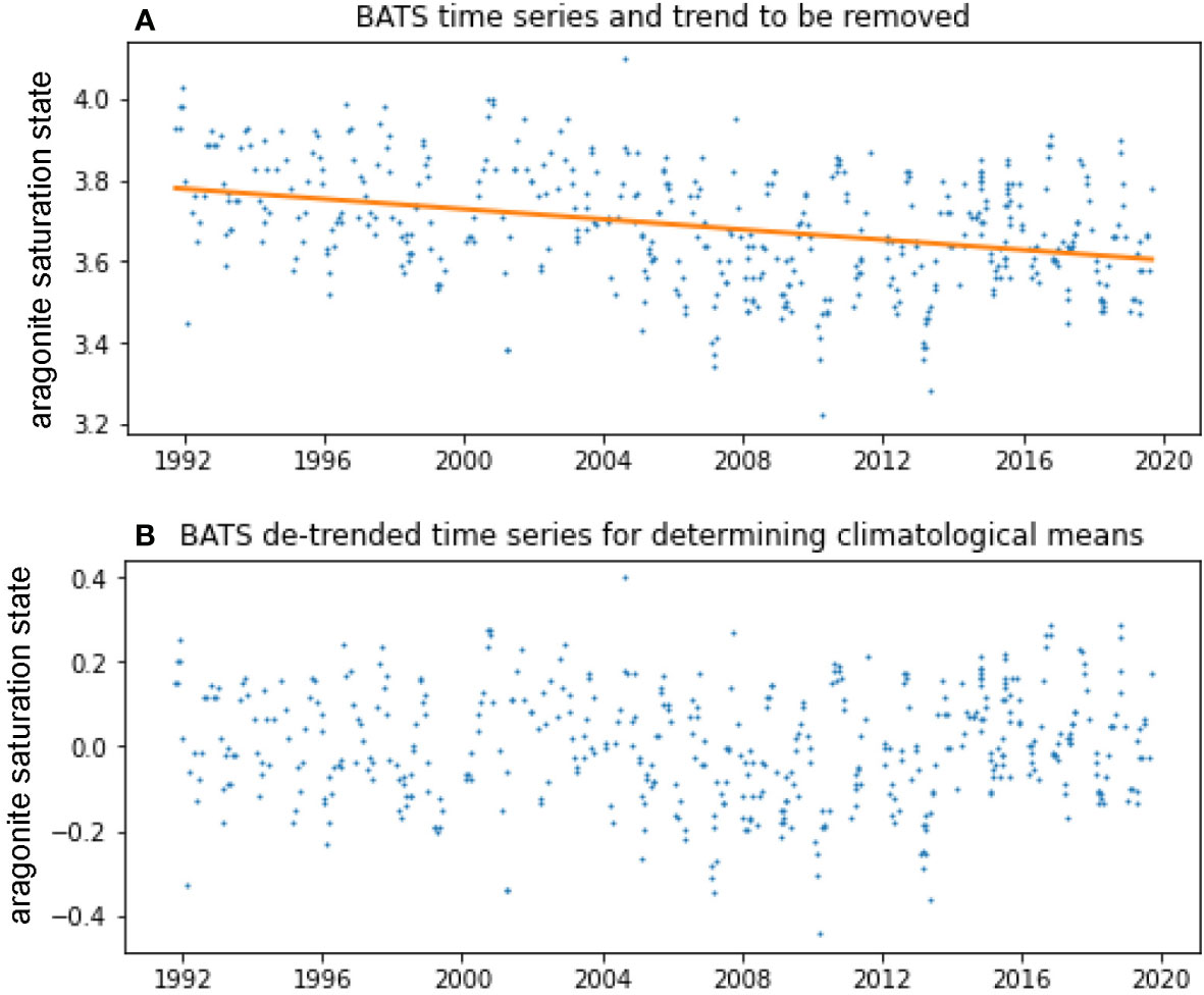
Figure 3 (A) Bermuda Atlantic Time-series Study (BATS) surface (< 10 m depth) aragonite saturation state (blue) calculated using measurements of temperature, salinity, inorganic nutrients, DIC, and TA in PyCO2SYS (Humphreys et al., 2022) with the constants recommended by Orr et al. (2018) and the associated linear trend (orange). (B) The same time series with the trend removed (shown as anomalies around zero), which is used for calculating monthly adjustments (Figure 4) that remove the seasonal cycle from the time series of monthly means.

To characterize and remove a seasonal cycle, we generate and apply monthly adjustments to a time series of monthly means. First, the monthly adjustments are determined by the difference between the climatological monthly means and the climatological annual mean (the mean of the climatological monthly means) of the de-trended data (Figure 3B). Examples of these monthly adjustments are shown in Figure 4. Using the original data set, we then develop a time series of monthly means and apply the monthly adjustments, producing a time series of monthly anomalies with the seasonal cycle removed (i.e., de-seasoned monthly means). This steps produce a time series of de-seasoned monthly values with a magnitude similar to the climatological mean as in Takahashi et al. (2009) rather than anomalies centered around zero as in Bates (2001). The Takahashi et al. (2009) approach is chosen here as it produces values that may be more intuitive in the case that trends are presented to the public or decision makers. An example of the original time-series observations, monthly means, and de-seasoned monthly means are shown in Figure 5.

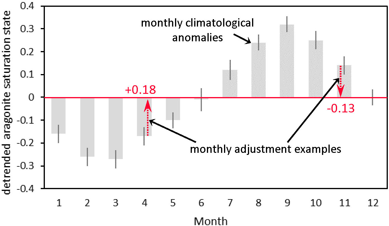
Figure 4 An example surface seawater aragonite saturation state monthly climatology from the Kuroshio Extension Observatory (KEO) mooring showing monthly mean (gray bars) and standard deviation (error bars) of de-trended values, shown as anomalies around zero, which represents the annual climatological mean (red solid line) as in Figure 3B. Two examples of the monthly adjustments are also shown for April (+0.18) and November (-0.13) derived from these climatologies. The adjustments will be applied to the time series of monthly means to remove the seasonal cycle. In practice, adjustments are calculated and applied for all twelve months.

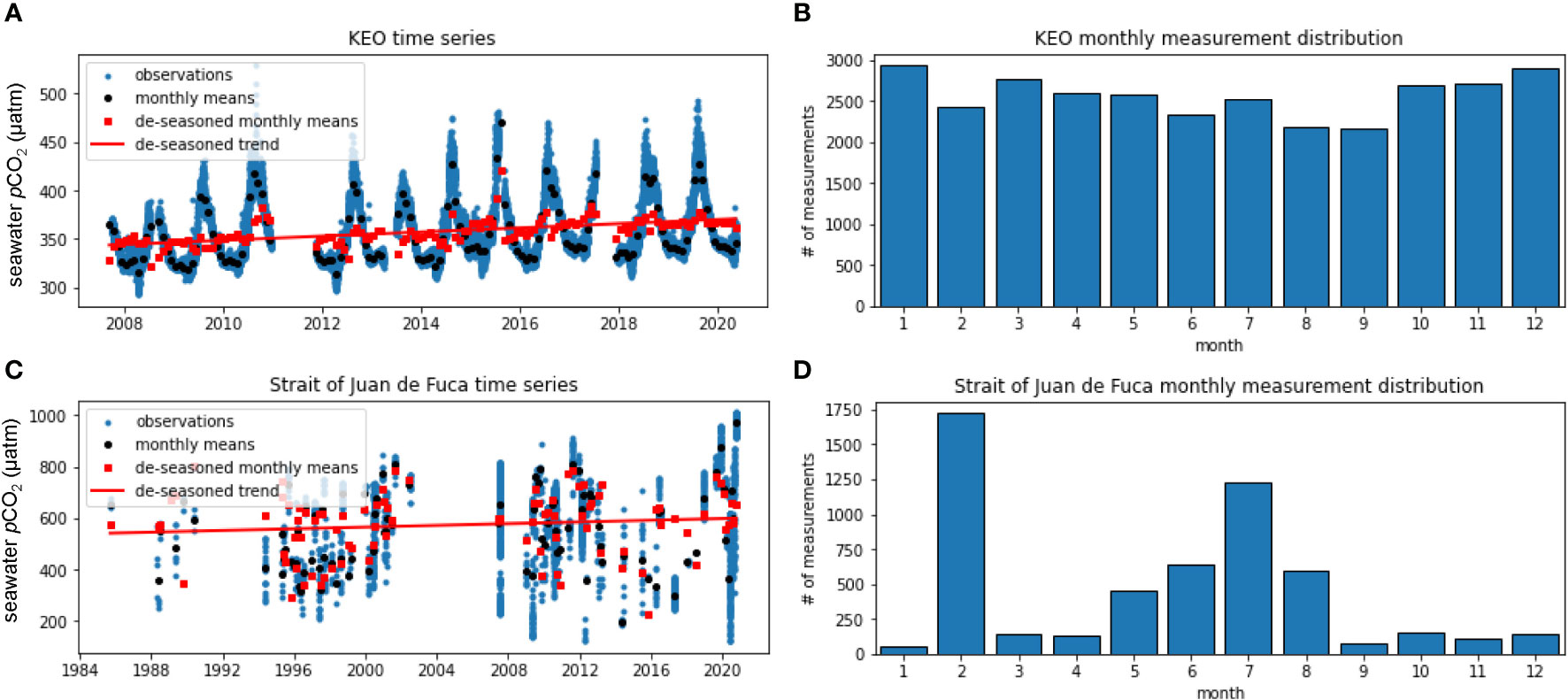
Figure 5 Surface seawater pCO₂ (µatm) from the KEO mooring (A) and ship-based underway measurements in the Strait of Juan de Fuca (C) including the original time-series observations (blue circles), the time series of monthly means (black circles), the de-seasoned monthly means (red squares), and the trend of the de-seasoned monthly means (red line). Monthly measurement distribution of the KEO (B) and Strait of Juan de Fuca (D) time series are also shown.

Monthly binning may not always be ideal. Shorter/smaller bins may allow for better resolution of seasonal extremes or recurring features that appear on sub-monthly timescales, but require more annual cycles to be resolved to ensure that non-periodic variations are not miscategorized as part of the seasonal cycle. Longer/larger bins may improve the statistics obtainable with infrequent measurements, but may fail to resolve the amplitude in the seasonal cycle. We nevertheless suggest reporting trends following the de-seasoning performed with monthly binning as by Bates (2001) and Takahashi et al. (2009) for comparability with other time-series assessments. However, other binning approaches that best suit the specific time series being considered should also be tested and reported.

If monthly adjustments were made when no significant seasonality exists, uncertainties in the monthly adjustments could rival the magnitudes of the adjustments themselves. For this reason, these best practices are best suited for time series collected in the surface and near surface where seasonal patterns occur. Future work should consider adjustments to these best practices to better constrain ocean interior change when there is a larger body of subsurface time series with sub-seasonal data collection to learn from.

3.3 Assess linear fit

We then apply a weighted least squares (WLS) method of linear regression to the time series of de-seasoned monthly means. The following assumptions are made in this analysis, including: 1) monthly means are normally distributed; 2) all data are subject to the same biases and have equal precision; and 3) autocorrelation is present in ocean biogeochemical time series. To account for the third assumption, the WLS method is used with Newey-West standard errors to provide improved estimates of the uncertainties of the linear regression coefficients by accounting for autocorrelation and heteroskedasticity in the data (Newey and West, 1987).

Figure 5 shows the resulting trend in the form of a time series based on the dates the observations were collected; however, we use a series of dates adjusted to start at 0 when applying the linear regression model. Using decimal year of the actual sample collection time instead would cause all the x-values to be distributed far from x=0, resulting in a y-intercept value that is highly sensitive to the input data. Changes to the data, such as adding another year of observations, could cause significant changes in the y-intercept because the of the increased uncertainty associated with extrapolation far beyond the range of the data. If the user plans to apply the linear regression equation with slope and y-intercept to predict biogeochemical values forward or backward in time, they must account for the x-values (in decimal years) beginning at the start of the time series at zero. This adjustment to the x-values does not change the slope, adjusted R², and other key statistics useful in the interpretation and statistical significance of the de-seasoned trend (Table 1).

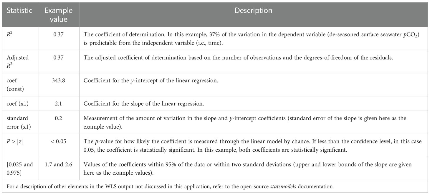
Table 1 A subset of statistics resulting from the WLS method of linear regression using the statsmodels Python package, including values generated by the example shown in Figure 5A and a description of each element.

Table 1 statistics suggest a significant trend in the de-seasoned monthly means derived from autonomous surface seawater pCO₂ record at the Kuroshio Extension Observatory (KEO) mooring. The slope coefficient is significant, the slope standard error is an order of magnitude less than the slope (2.1 ± 0.2 µatm yr^-1), and the linear regression describes 37% of variability in the data set. Using raw, high-frequency time series data rather than de-seasoned monthly means does not result in a significantly different trend in this case; however, it does reduce the adjusted R² from 0.37 to 0.07.

As part of these best practices, we recommend applying a linear fit to the entire de-seasoned data set for the purpose of consistent reporting across regions and research groups. However, there may be reasons to also consider the trends over different time periods within the data set. For example, to interrogate how different phases of the El Niño Southern Oscillation (ENSO) impact long-term change in the tropical Pacific, time series are commonly separated into El Niño, La Niña, and neutral time periods to assess trends in the different ENSO phases separately (Takahashi et al., 2003; Sutton et al., 2014). Trends over different seasons can also be interrogated and compared to help assess drivers of change (Park and Wanninkhof, 2012). For longer time series, decadal variability often influences long-term trends and can also be interrogated separately depending on the phases of the dominant climatic oscillations (e.g., Pacific Decadal Oscillation, Southern Annular Mode, North Atlantic Oscillation) in the ocean region of interest (Feely et al., 2006; Landschützer et al., 2016; Wanninkhof et al., 2019). It may also be important to present trends for different subsets of a time series based on changes in the operating parameters of the observing system, for example, to assess whether the apparent trend changed due to a change in observing methodology. These approaches can be done using the supplemental open-source software by uploading a data file with separate columns of data covering the different time periods and comparing the resulting trends.

3.4 Estimate trend detection time

In addition to the statistics describing the linear regression model (Table 1), trend detection time methodology is another statistical tool to help inform whether the trend signal is statistically detectable above the noise, which can often be substantial due to natural variability of ocean biogeochemistry. We use a statistical method described by Tiao et al. (1990) and first applied to environmental data by Weatherhead et al. (1998) to estimate the number of years of observations needed to detect a statistically significant trend. This method provides an assessment of the signal-to-noise ratio of the data but also factors in autocorrelation, which is a common feature of environmental data sets. Some applications of this methodology include determining when recovery of the ozone layer could be detected (Weatherhead et al., 2000) and when trends could be detected in satellite-based ocean color records (Henson et al., 2010; Henson et al., 2018) and ocean biogeochemical model output (Lovenduski et al., 2015).

To estimate the number of years of observations needed to detect a statistically significant trend, trend detection time (TDT), presented in years of observations, is determined by:

where σ_N is the standard deviation of monthly means that are de-seasoned and de-trended, ∅ is the autocorrelation (at lag 1, or one month lag) of the noise in the time series, and ω₀ is the slope determined by the WLS linear regression step. This results in a 90% probability (dictated by the factor of 3.3 in Eq. 1) of trend detection by the estimated TDT at the 95% confidence interval. This follows common practice that a trend is considered significant at the 95% confidence level if the magnitude is twice the standard deviation.

Uncertainty in TDT, u_TDT, is calculated by:

where B is the uncertainty factor calculated using the method of Weatherhead et al. (1998). Uncertainty is based on the number of months (m) in the time series and autocorrelation of de-seasoned monthly means (∅):

This application of the method analyses the noise in the time series and returns an estimate of the number of years of observations needed to detect the de-seasoned trend determined in Section 3.3. Characterizing and removing the seasonal signal in previous steps increases the signal-to-noise ratio (compared to the original data set), which reduces the resulting number of years of observations necessary to detect a trend. In an analysis of 40 autonomous seawater pCO₂ time series, Sutton et al. (2019) found TDT to be 55% shorter when using de-seasoned and de-trended monthly means compared to using raw, high-frequency time series data. In the example shown in Figure 4A and Table 1, de-seasoning the surface seawater pCO₂ data set as recommended in these best practices results in a TDT of 10.4 ± 2.5 years. The 12.7 year observing record at KEO has just approached this length threshold for the time series of de-seasoned monthly means.

If there are natural modes of variability that are not characterized by the data set, the resulting TDT may be an incorrect. This could occur when data are collected on a monthly basis in a region that exhibits large daily variability or extreme events or when a short time series is being analyzed from a region that exhibits large interannual or decadal variability (Sutton et al., 2019). This approach relies on first-order autoregression, meaning the immediately preceding monthly value is used to predict the present monthly value. The resulting TDT likely provides a minimum estimate of trend detection time given longer-term memory processes are important drivers of ocean carbon chemistry (Séférian et al., 2013).

In addition to removing the seasonal signal, there may be other ways to reduce TDT by adjusting the data set or modifying future data collection. The signal-to-noise ratio can be increased by improving measurement precision, which is another source of noise in all observational data sets. If the data set includes observations collected over a broad region (rather than a fixed-point time-series), natural spatial variability may also introduce noise to the time series, increasing the number of years of observations necessary to detect a trend. For example, there is not a significant trend in the 35-year data set of underway pCO₂ observations in the Strait of Juan de Fuca (Figure 5C). Natural spatial variability over this large region and low number of measurements during some months (Figure 5D) likely contribute to noise in this time series. The analysis suggests another decade of data may be necessary to detect a statistically-significant trend above this noise. In cases like this, the user may experiment with the size of the region of study while maintaining enough observations to characterize the seasonal signal and climatological annual mean.

3.5 Consider uncertainty

The initial assessment of data gaps (Section 3.1), statistics resulting from the WLS linear regression model (Section 3.3), and the trend detection time (Section 3.4) all provide information about uncertainty in the resulting trend. In the basic approaches used in these best practices, we assume that gaps in the data set do not impact the monthly mean climatology or annual climatological mean used to remove the seasonal cycle. If the data analyst believes the climatological gap-filling approach illustrated in Figure 2A does not adequately characterize monthly means, then additional research is necessary to identify the appropriate gap filling methods or the trend should only be considered over the months or seasons with repeated measurements (Figure 2B).

We also assume the monthly means are normally distributed and all the measurements in the time series are subject to the same biases and have equal precision. As discussed in Section 3.1, there may be instances where measurement bias or precision changes during the time series when measurement methods are modified. In cases with a known bias shift, the bias should be corrected in the data set prior to applying these best practices. There are also statistical techniques for propagating changes in measurement uncertainty within the linear regression statistics, but these are likely best considered on a case-by-case basis. In these cases, data analysts may be able to utilize consulting services available through statistics departments at universities and other research institutions or consult other resources such as Glover et al. (2011).

Given these assumptions are met, the WLS method statistics and trend detection time results provide evidence to assess whether the observed trend is statistically significant. At minimum, the standard error of the slope coefficient should be smaller than the value of the coefficient, the p-values for the coefficients should be less than the confidence level (i.e.,< 0.05), and the length of the time series should be longer than the estimated trend detection time.

3.6 Presentation of results

Uniform and transparent presentation of the results is critical. At minimum, we recommend statistically-significant ocean acidification trends be presented as change per year ± standard error. Trend results should be accompanied by a characterization of the temporal variability (e.g., magnitude of the diurnal and/or seasonal amplitude, inter-annual variability, etc.). In regional or global assessments, this is particularly important for providing stakeholders and other scientists context about local processes that drive variability (and impact trend assessments) across different ocean regions. We also recommend consistent reporting for carbon variables, including: DIC and TA on the gravimetric scale (µmol kg^-1); pH on the total scale; pCO₂, fCO₂, and pH at measurement temperature. The [H⁺] trend should be reported along with the trend in pH and the initial pH, which in the case of long-term trends, would be an annual mean of the first year of observations (Fassbender et al., 2020).

Results should also provide a clear explanation of what the trend represents in space and time. Even when using these methods, the detection of a statistically-significant trend does not imply the trend is a long-term trend of anthropogenic origin or that it does not represent competing and/or amplifying processes (Salisbury and Jönsson, 2018; Turk et al., 2019; Hauri et al., 2021). That assessment can only be made with an understanding of all modes of natural variability in the region and context for the changes that might be expected from atmospheric anthropogenic carbon accumulation. For example, these best practices produce an inter-annual or multi-decadal trend at a site that can then be compared to the rate of change assuming ocean acidification is progressing in equilibrium with the global atmospheric CO₂ increase (e.g., approximately -0.008 yr^-1 in surface ocean aragonite saturation state) or compared to a regionally-specific anthropogenic trend, if known. This emphasizes that variability and multi-decadal “trends” can reveal the processes impacting ocean carbon chemistry at a given location, which for coastal regions is often atmospheric CO₂ increase in addition to other natural processes and anthropogenic stressors. Spatial variability should also be considered, especially if the trends are computed on observations collected over a larger spatial footprint than a fixed-point time series. If information about spatial variability around the time-series location is known (e.g., Henson et al., 2016; Murphy et al., 2001; Jones et al., 2012), including an estimation of the spatial footprint of those variations is also useful context.

Presentation of results should also include metrics that are most relevant to the intended audience. For example, some stakeholders may require a trend to be presented as a change in seawater pH (e.g., UN SDG 14.3), whereas others may be more interested in a change in [H⁺]. In addition, some stakeholders and policy makers may not necessarily be interested in rates of change over time, but rather the point in time when a potential biological or ecological threshold is exceeded and/or when there is a detectable change in the frequency of exposure events. Trends resulting from these best practices can be applied backward and forward in time to examine and present when a threshold is projected to be crossed. However, projections should be presented with the understanding that trends are expected to vary over decades to centuries due to interannual variability, nonlinear atmospheric CO₂ changes, and the inherent nonlinearity of ocean carbonate chemistry. More research is needed to develop tools for characterizing exceeded thresholds or the changing frequency of “extreme” exposure events. Common statistical approaches for detecting frequency of signals in a time series, such as Fourier analysis, can only be applied to continuous data sets with regular sampling intervals.

4 Supporting code

These approaches are automated in the supplemental open-source software package fully documented and maintained on GitHub (https://github.com/NOAA-PMEL/TOATS). Data analysts do not need Python programming experience to run the code. The user needs to install Python, create and activate the environment, and open and run the Jupyter Notebook in a browser, all of which are described in detail on GitHub. The user also needs to create a data file that includes a column of datetimes and subsequent columns of values for the biogeochemical parameters of interest. When the program is run, a user interface will guide the file upload and ask the user to input the time-series name, file name, and the measurement uncertainty, units, and desired number of decimal places for each parameter. The program will generate a report including figures similar to those presented here, statistics described in Table 1, the estimate of the number of years of observations needed to detect a statistically significant trend, and a description of the time-series variability, trend, and associated uncertainties. The program will also export a file for each variable with the time series of de-seasoned monthly means generated by the code.

5 Conclusions

These best practices offer a basic but uniform analysis of trends that can be implemented on most data sets by GOA-ON, UN SDG, and WMO, and by individual scientists with an interest in comparing trends across a variety of regions. Every researcher must use their own knowledge of the system they are working in to determine additional time-series analyses needed to understand biogeochemical changes over time. Additional inquiries may be necessary in the time and space domain to determine the drivers of trends. Are trends during some seasons different from others? Are seasonal amplitudes or short-term extreme events increasing over time as buffer capacity decreases? What is the relative impact of warming seawater vs. anthropogenic CO₂ on ocean acidification trends? Will ocean acidification trends become nonlinear as atmospheric CO₂ forcing changes? These and many other questions may be worth pursuing above and beyond the approaches presented here.

These approaches for characterizing a time series are also useful for assessing how different observing strategies influence the ability to detect a trend. Sampling frequency, measurement uncertainty, and time-series length are all factors that contribute to the ability to detect a statistically-significant trend (Carter et al., 2019). Using this recommended sequence of approaches on observational data or model output can inform new sampling strategies and provide stakeholders with an estimate of when trends may be detectable over natural variability at a given location. Trend assessment can also highlight the value in managing time-series records in a way that reduces data gaps, manages changes in methodologies and data processing, and fully documents operating procedures. Those maintaining long-term ocean acidification time series should refer to guidance on how to best manage climate networks (Karl et al., 1995; Trenberth et al., 2002).

In conclusion, we acknowledge that as the community of practice in ocean carbon time-series analysis expands and research on ocean acidification trends progresses, it will be essential that the community revisit and update these best practices. Additional research is needed to determine whether other empirical or statistical techniques could be applied consistently across a variety of ocean and coastal time series to fill data gaps without introducing bias to the resulting trends. Research is also needed to better characterize the following: 1) periodic signals at frequencies other than seasonal, 2) changing frequency of extreme events, 3) changing variability as ocean buffer capacity decreases, 4) changing carbonate chemistry in low-salinity environments, and 5) the non-linear trend of pH over long time periods. Opportunities to explore these topics will grow as more publicly-available data sets, including high-frequency subsurface data sets, become available to support this research. We recommend that the organizations supporting coordination efforts within the ocean carbon and biogeochemistry community, such as GOA-ON and the International Ocean Carbon Coordination Project (IOCCP), support regular forums for sharing results and new techniques in trend analysis and modify these best practices accordingly.

Data availability statement

Publicly available datasets were analyzed in this study. These data can be found here: This study only utilized ocean acidification data sets that are publicly available, including from BATS at http://bats.bios.edu/bats-data, from NOAA’s moored time series (Sutton et al., 2019), and from SOCAT (Bakker et al., 2016; www.socat.info/index.php/data-access). The supplemental code is open-access and fully documented on GitHub at [https://github.com/NOAA-PMEL/TOATS].

Author contributions

AS and JN identified the need for these best practices and organized the initial workshop. AS took the lead in writing the manuscript with substantial contributions from BC and WE in early drafts. AS and RB developed the supplemental code, and BC, WE, RW, and BT tested the supplemental code. All authors provided critical feedback and helped shape the research, analysis, and manuscript. All authors read and approved the final manuscript.

Funding

NOAA’s Ocean Acidification Program and the Global Ocean Acidification Observing Network.

Acknowledgments

We acknowledge NOAA’s Ocean Acidification Program and the Global Ocean Acidification Observing Network for funding the Ocean Acidification Time-Series Analysis Workshop in February 2020 that served as the foundation for this work. We are greatly appreciative of the invited speakers of that workshop, Pieter Tans of NOAA’s Earth System Research Laboratories and Peter Guttorp of the Norwegian Computing Center and the University of Washington, who provided key insights into the standards and statistical approaches taken by the atmospheric community. We also thank additional attendees who provided feedback during a remote session in which recommendations were presented to a broader audience: Dorothee Bakker, Dwight Gledhill, Burke Hales, Peter Landschüster, Kathy Tedesco, and Nico Lange, who also provided feedback on the time series locations in Figure 1. This is PMEL contribution 5426.

Conflict of interest

The authors declare that the research was conducted in the absence of any commercial or financial relationships that could be construed as a potential conflict of interest.

Publisher’s note

All claims expressed in this article are solely those of the authors and do not necessarily represent those of their affiliated organizations, or those of the publisher, the editors and the reviewers. Any product that may be evaluated in this article, or claim that may be made by its manufacturer, is not guaranteed or endorsed by the publisher.

References

Adelsman H., Binder L. W.(Eds.) (2012). Washington State Blue Ribbon Panel on Ocean Acidification Ocean acidification: From knowledge to action, Washington state’s strategic response (Olympia, Washington: Washington Department of Ecology).
Bakker D. C. E., Pfeil C. S., Landa N., Metzl K. M., O'Brien A., Olsen K., et al. (2016). A multi-decade record of high-quality fCO2 data in version 3 of the surface ocean CO2 atlas (SOCAT). Earth Syst. Sci. Data 8, 383–413. doi: 10.5194/essd-8-383-2016
Bates N. R. (2001). Interannual variability of oceanic CO2 and biogeochemical properties in the Western north Atlantic subtropical gyre. Deep Sea Res. Part II: Topical Stud. Oceanogr. 48, 1507–1528. doi: 10.1016/S0967-0645(00)00151-X
Bates N. R., Astor M. J., Church K., Currie J. E., Dore M., González-Dávila L., et al. (2014). A time-series view of changing ocean chemistry due to ocean uptake of anthropogenic CO2 and ocean acidification. Oceanogr. 27, 126–141. doi: 10.5670/oceanog.2014.16
Bates N. R., Mathis J. T., Cooper L. W. (2009). Ocean acidification and biologically induced seasonality of carbonate mineral saturation states in the western Arctic ocean. J. Geophys. Res. C11007, 114. doi: 10.1029/2008JC004862
Boyer T., Zhang H.-M., O'Brien K., Reagan J., Diggs S., Freeman E., et al. The effects of the pandemic on the ocean observing system. Bull. Am. Meteorol. Soc.
Cai W.-J., Feely R. A., Testa J. M., Li M., Evans W., Alin S. R., et al. (2021). Natural and anthropogenic drivers of acidification in Large estuaries. Ann. Rev. Mar. Sci. 13, 23–55. doi: 10.1146/annurev-marine-010419-011004
Carter B. R., Williams N. L., Evans W., Fassbender A. J., Barbero L., Hauri C., et al. (2019). Time-of-detection as a metric for prioritizing between climate observation quality, frequency, and duration. Geophys. Res. Lett. 46, 3853–3861. doi: 10.1029/2018GL080773
Chan F., Boehm A. B., Barth J. A., Chornesky E. A., Dickson A. G., Feely R. A., et al. (2016). The West coast ocean acidification and hypoxia science panel: Major findings, recommendations, and actions (Oakland, California, USA: California Ocean Science Trust).
Chan F., Barth J. A., Blanchette C. A., Byrne R. H., Chavez F., Cheriton O., et al. (2017). Persistent spatial structuring of coastal ocean acidification in the California current system. Sci. Rep. 7, 2526. doi: 10.1038/s41598-017-02777-y
Dickson A. G. (1990). Standard potential of the reaction: AgCl(s) + 1/2 H2(g) = ag(s) + HCl(aq), and the standard acidity constant of the ion HSO4– in synthetic sea water from 273.15 to 318.15 K. J. Chem. Thermodynam. 22, 113–127. doi: 10.1016/0021-9614(90)90074-Z
Dickson A. G., Sabine C. L., Christian J. R. (Eds.) (2007). Guide to best practices for ocean CO2 measurements. north pacific marine science organization North Pacific Marine Science Organization, 176 pp.
Doney S. C., Busch D. S., Cooley S. R., Kroeker K. J. (2020). The impacts of ocean acidification on marine ecosystems and reliant human communities. Annu. Rev. Environ. Resour. 45, 1, 83–1,112. doi: 10.1146/annurev-environ-012320-083019
Fassbender A. J., Orr J. C., Dickson A. G. (2020). Technical note: Interpreting pH changes. Biogeosci. Discuss. 2020, 1407–1415. doi: 10.5194/bg-2020-348
Feely R. A., Takahashi T., Wanninkhof R., McPhaden M. J., Cosca C. E., Sutherland S. C., et al. (2006). Decadal variability of the air-sea CO2 fluxes in the equatorial pacific ocean. J. Geophys. Res. 111, C08S90. doi: 10.1029/2005JC003129
Franco A. C., Ianson D., Ross T., Hamme R. C., Monahan A. H., Christian J. R., et al. (2021). Anthropogenic and climatic contributions to observed carbon system trends in the northeast pacific. Global Biogeochem.Cycles 35. doi: 10.1029/2020GB006829
Friis K., Körtzinger A., Wallace D. W. R. (2003). The salinity normalization of marine inorganic carbon chemistry data. Geophys. Res. Lett. 30, 1085. doi: 10.1029/2002GL015898
Gattuso J.-P., Magnan A., Billé R., Cheung W. W. L., Howes E. L., Joos F., et al. (2015). Contrasting futures for ocean and society from different anthropogenic CO2 emissions scenarios. Science 349 (6243), aac4722. doi: 10.1126/science.aac4722
Glover D. M., Jenkins W. J., Doney S. C. (2011). Modeling methods for marine science (New York: Cambridge University Press).
GOA-ON (2019) Global ocean acidification observing network (GOA-ON) implementation strategy 2019. Available at: www.goa-on.org.
Hauri C., Pagès R., McDonnell A.M.P., Stuecker M.F., Danielson S.L., Hedstrom K., et al. (2021). Modulation of ocean acidification by decadal climate variability in the gulf of Alaska. Commun. Earth Environ. 2, 191. doi: 10.1038/s43247-021-00254-z
Henson S. A., Beaulieu C., Lampitt R. (2016). Observing climate change trends in ocean biogeochemistry: when and where. Glob. Change Biol. 23 (4), 1561–1571. doi: 10.1111/gcb.13152
Henson S. A., Cole H. S., Hopkins J., Martin A. P., Yool A. (2018). Detection of climate change-driven trends in phytoplankton phenology. Glob. Change Biol. 24, e101–e111. doi: 10.1111/gcb.13886
Henson S. A., Sarmiento J. L., Dunne J. P., Bopp L., Lima I., Doney S. C., et al. (2010). Detection of anthropogenic climate change in satellite records of ocean chlorophyll and productivity. Biogeosciences 7, 621–640. doi: 10.5194/bg-7-621-2010
Humphreys M. P., Lewis E. R., Sharp J. S., Pierrot D. (2022). PyCO2SYS v1.8: marine carbonate system calculations in Python. Geosci. Model. Dev. 15, 15–43. doi: 10.5194/gmd-15-15-2022
Jiang L.-Q., Cai W.-J., Wanninkhof R., Wang Y., Lüger H. (2008). Air-sea CO2 fluxes on the U.S. south Atlantic bight: Spatial and seasonal variability. J. Geophys. Res. 113, C07019. doi: 110.1029/2007jc004366
Jones S. D., Le Quéré C., Rödenbeck C. (2012). Autocorrelation characteristics of surface ocean pCO2and air-sea CO2 fluxes. Global Biogeochem. Cycles 26, GB2042. doi: 10.1029/2010GB004017
Karl T. R., Derr V.E., Easterling D.R., Folland C.K., Hofmann D.J., Levitus S., et al. (1995). Critical issues for long-term climate monitoring. Climatic Change 31, 185–221. doi: 10.1007/BF01095146
Kwiatkowski L., Orr J. C. (2018). Diverging seasonal extremes for ocean acidification during the twenty-first century. Nat. Climate Change 8, 141–145. doi: 10.1038/s41558-017-0054-0
Landschützer P., Gruber N., Bakker D. C. E. (2016). Decadal variations and trends of the global ocean carbon sink. Global Biogeochem. Cycles 30, 1396–1417. doi: 10.1002/2015GB005359
Lauvset S. K., Lange N., Tanhua T., Bittig H. C., Olsen A., Kozyr A., et al. (2021). An updated version of the global interior ocean biogeochemical data product, GLODAPv2.2021. Earth Syst. Sci. Data 13 (12), 5565–5589. doi: 10.5194/essd-13-5565-2021
Lee K., Kim T.-W., Byrne R. H., Millero F. J., Feely R. A., Liu Y.-M. (2010). The universal ratio of boron to chlorinity for the north pacific and north Atlantic oceans. Geochim. Cosmochim. Acta 74, 1801–1811. doi: 10.1016/j.gca.2009.12.027
Lovenduski N. S., Long M. C., Lindsay K. (2015). Natural variability in the surface ocean carbonate ion concentration. Biogeosciences 12, 6321–6335. doi: 10.5194/bg-12-6321-2015
Lueker T. J., Dickson A. G., Keeling C. D. (2000). Ocean pCO2 calculated from dissolved inorganic carbon, alkalinity, and equations for K1 and K2: validation based on laboratory measurements of CO2 in gas and seawater at equilibrium. Mar. Chem. 70, 105–119. doi: 10.1016/S0304-4203(00)00022-0
Masarie K. A., Tans P. P. (1995). Extension and integration of atmospheric carbon dioxide data into a globally consistent measurement record. J. Geophys. Res. 100, 11593–11610. doi: 10.1029/95JD00859
Ministry of Environment and Climate Change Strategy (2019). Preliminary strategic climate risk assessment for British columbia. report prepared for the government of British Columbia, Victoria, BC. Available at: https://www2.gov.bc.ca/gov/content/environment/climate-change/adaptation/riskassessment.
Mongin M., Baird M. E., Tilbrook B., Matear R. J., Lenton A., Herzfeld M., et al. (2016). The exposure of the great barrier reef to ocean acidification. Nat. Commun. 7, 10732. doi: 10.1038/ncomms10732
Murphy P. P., Nojiri Y., Harrison D. E., Larkin N. K. (2001). Scales of spatial variability for surface ocean pCO2 in the gulf of Alaska and Bering Sea: Toward a sampling strategy, geophys. Res. Lett. 28, 1047–1050. doi: 10.1029/2000GL012375
Newey W. K., West K. D. (1987). A simple, positive semi-definite, heteroskedasticity and autocorrelation consistent covariance matrix. Econometrica 55, 703–708. doi: 10.2307/1913610
Orr J. C., Epitalon J.-M., Dickson A. G., Gattuso J.-P. (2018). Routine uncertainty propagation for the marine carbon dioxide system. Mar. Chem. 207, 84–107. doi: 10.1016/j.marchem.2018.10.006
Park G.-H., Wanninkhof R. (2012). A large increase of the CO2 sink in the western tropical north Atlantic from 2002 to 2009. J. Geophys. Res. 117, C08029. doi: 10.1029/2011JC007803
Riebesell U., Fabry V. J., Hansson L., Gattuso J.-P. (2011). Guide to best practices for ocean acidification research and data reporting (Luxembourg: Publications Office of the European Union), 260 pp.
Salisbury J. E., Jönsson B. F. (2018). Rapid warming and salinity changes in the gulf of Maine alter surface ocean carbonate parameters and hide ocean acidification. Biogeochemistry 141, 401–418. doi: 10.1007/s10533-018-0505-3
Schockman K. M., Byrne R. H. (2021). Spectrophotometric determination of the bicarbonate dissociation constant in seawater. Geochim. Cosmochim. Acta 300, 231–245. doi: 10.1016/j.gca.2021.02.008
Séférian R., Bopp L., Swingedouw D., Servonnat J. (2013). Dynamical and biogeochemical control on the decadal variability of ocean carbon fluxes. Earth Syst. Dynam. 4, 109–127. doi: 10.5194/esd-4-109-2013
Sutton A. J., Feely R. A., Sabine C. L., McPhaden M. J., Takahashi T., Chavez F. P., et al. (2014). Natural variability and anthropogenic change in equatorial pacific surface ocean pCO2 and pH. global biogeochemical cycles. Earth System Science Data 28, 131–145. doi: 10.1002/2013GB004679
Sutton A. J., Feely R.A., Maenner-Jones S., Musielwicz S., Osborne J., Dietrich C., et al. (2019). Autonomous seawater pCO2 and pH time series from 40 surface buoys and the emergence of anthropogenic trends. Earth Syst. Sci. Data 11, 421–439. doi: 10.5194/essd-11-421-2019
Sutton A. J., Newton J. A. (2020). Reaching consensus on assessments of ocean acidification trends. EOS 101. doi: 10.1029/2020EO150944
Takahashi T., Sutherland S. C., Sweeney C., Poisson A., Metzl N., Tilbrook B., et al. (2002). Global sea–air CO2 flux based on climatological surface ocean pCO2, and seasonal biological and temperature effects. Deep Sea Res. Part II: Topical Stud. Oceanogr. 49, 1601–1622. doi: 10.1016/S0967-0645(02)00003-6
Takahashi T., Sutherland S. C., Wanninkhof R., Sweeney C., Feely R.A., Chipman D. W., et al. (2009). Climatological mean and decadal change in surface ocean pCO2, and net sea-air CO2 flux over the global oceans. Deep Sea Res. Part II: Topical Stud. Oceanogr. 56, 554–577. doi: 10.1016/j.dsr2.2008.12.009
Takahashi T., Sutherland S. C., Feely R. A., Cosca C. E. (2003). Decadal variation of the surface water PCO2 in the Western and central equatorial pacific. Science 302, 852–856. doi: 10.1126/science.1088570
Tiao G. C., Reinsel G. C., Xu D., Pedrick J. H., Zhu X., Miller A. J., et al. (1990). Effects of autocorrelation and temporal sampling schemes on estimates of trend and spatial correlation. J. Geophys. Res. 95, 20507–20517. doi: 10.1029/JD095iD12p20507
Trenberth K. E., Karl T. R., Spence T. W. (2002). The need for a systems approach to climate observations. Bull. Am. Meteorol. Soc. 83, 1593–1602. doi: 10.1175/BAMS-83-11-1593
Tsutsumi Y., Mori K., Hirahara T., Ikegami M., Conway T. J. (2009). Technical report of global analysis method for major greenhouse gases by the world data center for greenhouse gases. WMO TD no. 1473 (Geneva: World Meteorological Organization) 29.
Turk D., Wang H., Hu X., Gledhill D. K., Wang Z. A., Jiang L., et al. (2019). Time of emergence of surface ocean carbon dioxide trends in the north American coastal margins in support of ocean acidification observing system design. Front. Mar. Sci. 6. doi: 10.3389/fmars.2019.00091
Vance J. M., Currie K., Zeldis J., Dillingham P. W., Law C. S. (2022). An empirical MLR for estimating surface layer DIC and a comparative assessment to other gap-filling techniques for ocean carbon time series. Biogeosciences 19, 241–269. doi: 10.5194/bg-19-241-2022
Wanninkhof R., Triñanes J., Park G. -H., Gledhill D., Olsen A. (2019). Large Decadal changes in air-Sea CO2 fluxes in the Caribbean Sea. J. Geophys. Res.: Oceans 124, 6960–6982. doi: 10.1029/2019JC015366
Waters J., Millero F. J., Woosley R. J. (2014). Corrigendum to “The free proton concentration scale for seawater pH”, [MARCHE: 149 (2013) 8–22]. Mar. Chem. 165, 66–67. doi: 10.1016/j.marchem.2014.07.004
Weatherhead E. C., Reinsel G. C., Tiao G. C., Meng X. -L., Choi D., Cheang W. -K., et al. (1998). Factors affecting the detection of trends: Statistical considerations and applications to environmental data. J. Geophys. Res.: Atmospheres 103, 17149–17161. doi: 10.1029/98JD00995
Weatherhead E. C., Reinsel G. C., Tiao G. C., Jackman C. H., Bishop L., Frith S. M. H., et al. (2000). Detecting the recovery of total column ozone. J. Geophys. Res.: Atmospheres 105, 22201–22210. doi: 10.1029/2000JD900063
Weisberg S. B., Bednaršek N., Feely R. A., Chan F., Boehm A. B., Sutula M., et al. (2016). Water quality criteria for an acidifying ocean: Challenges and opportunities for improvement. Ocean Coast. Manage. 126, 31–41. doi: 10.1016/j.ocecoaman.2016.03.010
Keywords: best practices, ocean acidification, biogeochemistry, trends, time series
Citation: Sutton AJ, Battisti R, Carter B, Evans W, Newton J, Alin S, Bates NR, Cai W-J, Currie K, Feely RA, Sabine C, Tanhua T, Tilbrook B and Wanninkhof R (2022) Advancing best practices for assessing trends of ocean acidification time series. Front. Mar. Sci. 9:1045667. doi: 10.3389/fmars.2022.1045667
Received: 15 September 2022; Accepted: 05 December 2022;
Published: 22 December 2022.
Edited by:
Jay S. Pearlman, Institute of Electrical and Electronics Engineers, FranceReviewed by:
Elise Olson, Princeton University, United StatesElizabeth Joan Drenkard, Princeton University, United States
Maribel I. García-Ibáñez, Institut de Ciències del Mar (ICM-CSIC), Spain
Copyright © 2022 Sutton, Battisti, Carter, Evans, Newton, Alin, Bates, Cai, Currie, Feely, Sabine, Tanhua, Tilbrook and Wanninkhof. This is an open-access article distributed under the terms of the Creative Commons Attribution License (CC BY). The use, distribution or reproduction in other forums is permitted, provided the original author(s) and the copyright owner(s) are credited and that the original publication in this journal is cited, in accordance with accepted academic practice. No use, distribution or reproduction is permitted which does not comply with these terms.
*Correspondence: Adrienne J. Sutton, adrienne.sutton@noaa.gov