Instance-based transfer learning for soil organic carbon estimation

1 Introduction

Soil organic carbon (SOC) is an essential part of the global carbon cycle (Bruhwiler et al., 2018) and one of the most significant soil parameters. It is the main element present in the soil organic matter (SOM), the significant nutrient source for crop yields, which is crucial to agricultural production (Obalum et al., 2017). SOC is a major source of terrestrial carbon and a pivotal element for soil quality and fertility, representing an important element of terrestrial ecosystems due to its great potential to affect the climate, food security, and agricultural sustainability. Soils contain approximately double of the world’s organic carbon compared to the amount present in the atmosphere (Schmidt et al., 2011). However, SOC has been found to sink in many regions, whereas atmospheric CO₂ permanently increases. It is well known that there is an obvious linkage between SOC and climate (Horwath and Kuzyakov, 2018). New studies have shown that changes in land use and land management practice can affect SOC stocks more than climatic changes (Niu et al., 2021).

Measuring and assessment of the soil components and properties is generally a time-consuming and costly procedure. The absence of measured data can be reimbursed by results of predictions or modeling (Kovačević et al., 2010). A commonly used approach to the estimation of not-supplied soil parameters is more conducted on their indirect assessment based on measures of the values of some other already available parameters.

The spatial distribution of soil variables is usually realized by predictive soil mapping that presents a numerical or statistical model of the relationship among environmental variables and soil properties, which is then applied to a geographic database to create a predictive map (Scull et al., 2003). Most of those models are based on geostatistical or regression methods (McBratney et al., 2003). The increasing richness and accessibility of different data sources led to attempts to enrich the soil information through the use of ancillary data (McBratney et al., 2000). In the early age of digital soil mapping, the co-kriging geostatistical method was developed for predicting a target soil variable based on subsidiary variables that are cheaper or quicker to measure and well correlated with the target one (McBratney and Webster, 1983).

The other approach to the estimation of soil properties is based on a pedotransfer function (PTF) that presents a mathematical model used to convert direct soil measurements into known and unknown soil properties (Bouma, 1989). Since most soil properties are interdependent, PTF is widely used for modeling relationships in soil research, hydrology, environmental science, etc. Most PTFs are developed to predict soil properties for a geographical area with limited information available (McBratney et al., 2002).

In the last decades, machine learning (ML) techniques have taken a very important role in the Spatio-temporal modeling of geochemical variables, especially in their stock assessment and dynamic changes (Wadoux et al., 2020; Heuvelink et al., 2021). Most of those studies are primarily focused on mapping soil properties or classes from local to regional and even worldwide scales by using different ML algorithms (Taghizadeh-Mehrjardi et al., 2016; Hengl et al., 2017; Estévez et al., 2022). The final outputs are mainly digital soil maps (DSM) produced by different ML algorithms. As a consequence, the main goals of researchers were to model soil properties in space and time by reaching satisfactory prediction accuracy without obtaining new knowledge on the core soil structure and process (Wadoux et al., 2020).

In recent years, ML was also applied for developing PTFs in different environmental studies: Benke et al. (2020) developed generalized PTF to predict soil electrical conductivity and SOC content for regional locations in the state of Victoria, Australia; Ramcharan et al. (2017) developed PTF using the Random Forest algorithm to fill in data gaps for SOC stock volumetric assessments across the US; Gunarathna et al. (2019) use different ML algorithms to develop PTF for available water content in tropical regions. All these studies mainly deal with the estimation of soil properties within the same geographical space, which implies similar or the same environmental conditions.

Traditional SOC measurements are time-consuming and laborious. Therefore, using ML to obtain SOC values based on other geochemical parameters could be the direction of future development. SOC concentration depends on various factors such as soil type, climate, topography, and soil management practices. SOC is greatly influenced by vegetation through the organic matter input and consequently, land use change is one of the most important factors which impacts SOC stock increase/decrease. Padarian et al. (2020) found that studies related to SOC cycles and dynamics and the estimation of SOC stocks in different ecosystems, with particular importance on grasslands and topsoil, were one of the main topics that preoccupied researchers who used ML techniques in soil science. Other recent geosciences studies indicate that the application of ML techniques was boosted with the increasing implementation of remote sensing techniques that enabled a significant extension of attribute space in the modeling process (Kovačević et al., 2009; Bouasria et al., 2022). Recently published studies indicate the efficient application of ML in combination with remote sensing and open access data in precision and smart agriculture management (Benos et al., 2021; Mahmood et al., 2022a,b).

Despite the increased number of predictors, there is still a lack of in situ collected data in geosciences disciplines that are essential for model building. As a possible solution to resolve this problem, the concept of transfer learning was suggested. Transfer learning (TL), as a sub-field of ML, adjusts a model developed for one learning task to be used as the starting point for building a model in another learning task (Tan et al., 2018). This technique is already used in environmental studies. Xiong et al. (2021) used TL on different satellite data for identifying pre-earthquake ionospheric perturbation before earthquakes to improve the performance of earthquake prediction. The application of TL has already been investigated in soil science. So far, researchers were focused on its application in soil spectroscopy. Liu et al. (2018) used neural network-based TL for soil spectroscopy and its performance on soil clay content estimation using hyperspectral data. Padarian et al. (2019) applied TL to improve a localized general soil spectral calibration model generated with a continental LUCAS dataset. TL aims to use the knowledge learned from previous tasks, or from large datasets, to solve new related tasks with limited data (Pan and Yang, 2010). Mallavan et al. (2010) introduced a procedure for identifying areas with similar soil forming factors seeking the smallest taxonomic distance between the factors of the region of interest (lacking in soil data) and other reference areas (with soil data) to export soil-landscape rules between those regions. A similar concept was used to detect Areas of Applicability estimated by the dissimilarity index. This index is based on the minimum multivariate distance calculation to the training data in the multidimensional predictor space (Meyer and Pebesma, 2021; Ludwig et al., 2022). Malone et al. (2016) elaborated a similar approach to extrapolate data across a large mapping area with sparsely measured points, called recipient site, from a nearby donor site (usually of a smaller spatial extent) with very detailed soil mapping.

The goal of this research is to investigate how an ML model, which estimates SOC values (output) in arable cropland by using geochemical and physical characteristics of the cropland soil samples (inputs), can be improved with a TL approach. Commonly, an ML model is built using the inputs and associated outputs in one (source) domain, and then applied in the other (target) domain where only the inputs are available. As opposed to this procedure, we propose to build the model not only on the inputs and outputs of the source domain but also to utilize the available inputs from the target domain. The instance-based TL approach assumes the difference between the underlying probability distributions of source and target domain samples described with geochemical and physical inputs. In this paper, two types of different but related source domains were examined: transfer from a global cropland domain to a local cropland domain and from a global grassland domain to a local cropland domain.

In the first part of section two, a description of the soil samples dataset is given. Basic theoretical foundations of the instance-based TL and Bhattacharyya distance are presented in the second part of section two. In section three, the model training process, the experimental setup, and the discussion of the results are given. Concluding remarks about the contribution and future research are presented in section four.

2 Materials and methods

2.1 LUCAS-based twelve countries soil organic carbon dataset

Following a decision of the European Parliament, the European Statistical Office (EUROSTAT), in close cooperation with the Directorate General responsible for Agriculture and the technical support of the Joint Research Centre (JRC), organizes regular, harmonized surveys across all EU Member States to gather information on land cover and land use. This survey is known as LUCAS - Land Use/Cover Area frame statistical Survey (Jones et al., 2020). In this paper, a data set from the year 2015 was used (the latest available release during the research). The 2015 LUCAS data set consists of 21,857 samples, with SOC measured following the ISO 10694:1995 protocol (Orgiazzi et al., 2018), and ranging from 0.10 to 560.20 g/kg, as shown in Figure 1 (in the original LUCAS data set, SOC is labeled as organic carbon (OC) content). The samples originate from 28 countries (EU member states) and are divided into eight land cover classes: grassland, shrubland, woodland, cropland, bareland, artificial land, wetlands, and water.

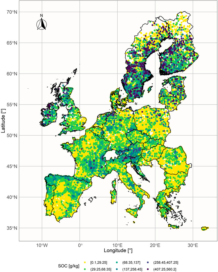
FIGURE 1. Spatial distribution of LUCAS samples and SOC values in [g/kg] for the year 2015.

The spatial variability of SOC depends on the climate and the share of land cover (i.e., vegetation type) across the EU. Organic carbon was the highest in the boreal zone, most of the Atlantic zone, and the temperate mountainous zone. It was intermediate in the sub-oceanic zone and lowest in the Mediterranean and sub-continental zones. Wetland, woodland, shrubland, and grassland were the main land cover (LC) classes in zones with the highest SOC values. On the contrary, cropland and bareland were the more common LC class in zones with the lowest SOC values (Jones et al., 2020). The lowest SOC values under arable land could be due to reduced inputs of organic matter and frequent tillage.

The proposed TL approach was evaluated on the subset of the LUCAS data set which consists of samples that 1) belong to the soil classes with similar geochemical characteristics and dissimilar SOC - cropland (relatively low), and grassland (relatively high); 2) come from the countries with at least 100 samples in each land class (12 countries). The cropland land cover class includes fields of cereal, root crops, industrial crops, dry pulses and vegetables, fodder crops, fruit trees, olive groves, and vineyards, while the grassland land cover class includes fields of grass with and without sparse trees below 1,000 m altitude (Jones et al., 2020). The subset is named LUCAS-12 and its statistical summary is presented in Table 1 and Figure 2.

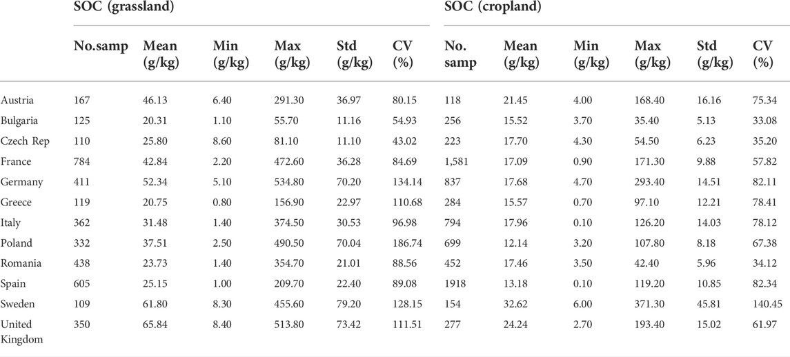
TABLE 1. LUCAS-12 dataset: summary statistics of SOC values per country and LC class.

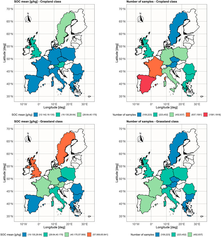
FIGURE 2. Spatial distribution of mean SOC values [g/kg], and number of samples aggregated per country in LUCAS-12 data set.

2.1.1 Explanatory variables for soil organic carbon estimation

The analysis of chemical and physical properties represents the core of the LUCAS Soil survey. According to Jones et al. (2020), a composite sample of approximately 500 g was taken from five subsamples collected with a spade at each LUCAS point. The first subsample was collected at the geo-referenced point location; the other four subsamples were collected at a distance of 2 m following the cardinal directions (North, East, South, and West).

In this research, five chemical and physical properties, measured at identical locations, were used as explanatory variables for SOC estimation: Nitrogen (Total Nitrogen concentration in g/kg for $<$ 2 mm soil fraction - labeled on figures as n_tot), pH - H₂O (1:1 Soil-Water Suspension for $<$ 2 mm soil fraction - ph_h20), pH - CaCl₂ (pH, CaCl₂ Suspension for $<$ 2 mm soil fraction - ph_cacl2), Potassium (Extractable in mg/kg for $<$ 2 mm soil fraction - k_ext), and Electrical Conductivity (Saturation Extract in dS/m for $<$ 2 mm soil fraction - ex_satp). All explanatory variables represent interconnected elements or indicators related to plant nutrition. The spatial distribution of explanatory variables is shown in Figure 3.

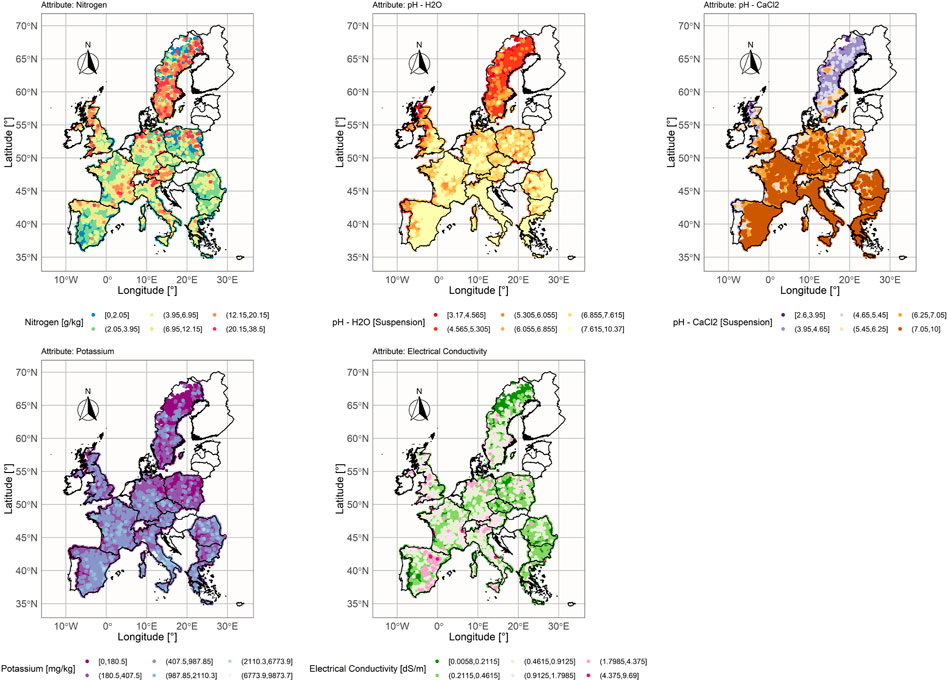
FIGURE 3. Spatial distribution of explanatory variables in a LUCAS-12 data set.

Pearson correlation coefficient, calculated between explanatory variables and SOC for the LUCAS-12 data set (Figure 4), showed that SOC values are highly correlated with Nitrogen values in both LC classes $(\ge 0.89)$. This finding is in accordance with (Jones et al., 2020). Moreover, the SOC-to-Nitrogen ratio is relatively stable across different soil types. Overall, mineral soils generally have a SOC-to-Nitrogen ratio close to 12:1, while organic-rich soils have a SOC-to-Nitrogen ratio close to 30:1 (Jones et al., 2020). There is a significant correlation between Electrical Conductivity and SOC in the grassland class.

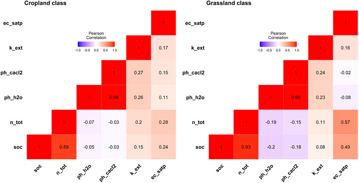
FIGURE 4. Correlation matrix as a heatmap between explanatory variables and soil organic carbon per land cover class.

2.2 Methodology

2.2.1 Instance-based non-inductive transfer learning

The proposed model for estimating SOC is designed to use the instance-based non-inductive transfer learning (Yang et al., 2020). We first define the basic concepts of transfer learning. A domain $\mathbb{D}=\mathbb{D}(\mathcal{X},P_X)$ consists of two components: a feature space $\mathcal{X}$ from which samples $\mathbf{x}\in \mathcal{X}$ come from, and a marginal probability distribution P_X that produces each sample x (in ML terminology, explanatory variables are denoted as features). All samples are or can be transformed to vectors of real numbers $\mathbf{x}\in {\mathbb{R}}^n$. Given a domain of interest, one can perform a task $\mathbb{T}$ which consists of two components: a label space $\mathcal{Y}$, and an unknown predictive function $f:\mathcal{X}\to \mathcal{Y}$ for which y = f(x). In a regression task, $y\in \mathcal{Y}$ is a real number, while in a classification task it takes one of several discrete values (classification labels). Estimating SOC values from geochemical and physical characteristics of soil samples is a regression task. In a regression task, the real f remains unknown, but we can learn y = g(x) from the available data ${({\mathbf{x}}_i,y_i=f({\mathbf{x}}_i))}_{i=1\cdots N}$, hoping that g will approximate f outside of the training set well. Function g is selected from a predefined family of functions and is completely determined with its parameter vector θ (i.e., if $g(\mathbf{x})=w_0+{\sum }_{i=1}^n{w}_i{x}_i$ then θ = (w₀, w₁, …, w_n)). To learn g from the available data, one needs to find θ which minimizes the prediction error ${\sum }_{i=1}^{N}l({\mathbf{x}}_i,y_i,\mathit{\theta })$, where the loss function l(x, y, θ) estimates the error for each sample. In a regression task, commonly used loss function is $l(\mathbf{x},y,\mathit{\theta })={(g_{\mathit{\theta }}(\mathbf{x})-y)}^2$. Mathematically, the learning process on a training set can be described as:

Due to the noisy nature of measurements, a training set often contains different values of y for the same x. Therefore, an unknown f can be interpreted as an expectation E(y|x) defined over the probability distribution P(y|x). Hence, a task $\mathbb{T}$ is defined to be $\mathbb{T}=\mathbb{T}(\mathcal{Y},P_{Y|X})$.

In the context of transfer learning, there are two domains of interest, source domain ${\mathbb{D}}_s$ and target domain ${\mathbb{D}}_t$. They are represented with source-labeled and destination-labeled datasets where the labelling process is the outcome of two tasks ${\mathbb{T}}_s$ and ${\mathbb{T}}_t$: ${({\mathbf{x}}_{s_i},y_{s_i})}_{i=1\cdots N}$, where ${\mathbf{x}}_{s_i}{\in \mathcal{X}}_s,y_{s_i}{\in \mathcal{Y}}_s$, and ${({\mathbf{x}}_{t_i},y_{t_i})}_{i=1\cdots M}$, where ${\mathbf{x}}_{t_i}{\in \mathcal{X}}_t,y_{t_i}{\in \mathcal{Y}}_t$. According to Pan and Yang (2010), transfer learning can be defined as follows:

Definition 1: Given ${\mathbb{D}}_s,{\mathbb{T}}_s,{\mathbb{D}}_t$, and ${\mathbb{T}}_t$, transfer learning aims to imporve the learning of the predictive function f_t from the target domain, using the knowledge in ${\mathbb{D}}_s$ and ${\mathbb{T}}_s$, where ${\mathbb{D}}_s\ne {\mathbb{D}}_t$ or ${\mathbb{T}}_s\ne {\mathbb{T}}_t$.

From Definition 1 follows that a traditional machine learning setting arises when ${\mathbb{D}}_s={\mathbb{D}}_t$ and ${\mathbb{T}}_s={\mathbb{T}}_t$. However, the nature of the difference between the domains or between the tasks can be used to categorize different transfer learning settings. We now define the instance-based non-inductive transfer learning:

Definition 2: Let ${\mathcal{Y}}_s{=\mathcal{Y}}_t$ and $P_{Y|X}^s=P_{Y|X}^t$ (i.e., ${\mathbb{T}}_s={\mathbb{T}}_t$). If ${\mathcal{X}}_s{=\mathcal{X}}_t$ and $P_X^s\ne P_X^t$ (i.e., ${\mathbb{D}}_s\ne {\mathbb{D}}_t$), the learning setting becomes instance-based and non-inductive.

An instance-based non-inductive setting assumes the same feature and label spaces as well as the same underlying process that maps inputs to outputs in both domains. However, the marginal probability distributions of instances (samples) are different across domains. In this paper, we assume the marginal probability distributions of the observed samples are different across various land cover types. Therefore, this setting can be applied when one tries to predict cropland SOC values using both geochemical + physical and SOC values from grassland samples (source domain), and only geochemical + physical values from cropland samples (target domain). Now, we explain how one can find the optimal parameters of the target prediction model g_t ≈ f_t.

Suppose that ${\mathbb{D}}_s$, ${\mathbb{T}}_s$, and ${\mathbb{D}}_t$ are represented with ${({\mathbf{x}}_{s_i},y_{s_i})}_{i=1\cdots N}$, and ${({\mathbf{x}}_{t_i})}_{i=1\cdots M}$. We would like to find the optimal parameters ${\mathit{\theta }}_t^{*}$ of the target task prediction model under the assumption of the instance-based non-inductive setting. Using the empirical risk minimization framework (Vapnik, 1998), we minimize the following expectation:

where l(x, y, θ_t) is a loss function defined for the target task. Using the definition of mathematical expectation, Eq. 2 becomes:

From Definition 2 follows $P_{Y|X}^s=P_{Y|X}^t$, and after using the Bayes’ rule, we obtain $P_t(y|\mathbf{x})=\frac{P_t(\mathbf{x},y)}{P_t(\mathbf{x})}=P_s(y|\mathbf{x})=\frac{P_s(\mathbf{x},y)}{P_s(\mathbf{x})}$, and hence $P_t(\mathbf{x},y)=\frac{P_t(\mathbf{x})}{P_s(\mathbf{x})}{P}_s(\mathbf{x},y)$. Since ${\mathcal{X}}_s{=\mathcal{X}}_t$ and ${\mathcal{Y}}_s{=\mathcal{Y}}_t$ (Definition 2), Eq. 3 becomes:

Optimal parameters of the target model cannot be found by Eq. 4 since the expectation of the joint distribution in the source population is impossible to compute. The best we can do is to apply the empirical approximation to the training data by modifying Eq. 1:

Equation 5 suggests why this method is called “instance-based”. Each source domain instance is weighted in the loss function with the ratio $\frac{P_t(\mathbf{x})}{P_s(\mathbf{x})}$, meaning that if an instance is more probable to occur in the target domain, then the optimization process pays more attention to it. If the probability ratio is 1 for all source instances, then the loss function takes its standard form described with Eq. 1 – the target prediction model is equal to the model created only on source domain data (classical machine learning setting without transfer of knowledge). The probability ratio can be estimated using the rejection sampling-based method for correcting sample selection bias (Zadrozny, 2004). This method introduces a new binary random variable δ ∈ {0, 1}, which selects whether a sample will be accepted by the source domain or not: P_s(x) = P(x|δ = 1), and P_t(x) = P(x|δ = 0). The ratio can be calculated as follows:

Equation 6 suggests that the probability ratio is proportional to $\frac{1}{P(\delta =1|\mathbf{x})}$. Hence, one can treat the evaluation of the ratio as a binary classification problem in which a classifier is trained to predict the probability of a sample being from the source domain (P(δ = 1|x)), or the target domain (P(δ = 0|x)).

2.2.2 Bhattacharyya distance

In this research, Bhattacharyya Distance (Bhattacharyya, 1946) is used to estimate the amount of overlap between the source and target domains (distributions $P_X^s$ and $P_X^t$). Let P and Q are two discrete probability distributions over the same domain $\mathcal{X}$. The Bhattacharyya distance B(P, Q) measures the similarity between P and Q using the following equation:

Since ${\sum }_{x\in \mathcal{X}}P(x)=1$ and ${\sum }_{x\in \mathcal{X}}Q(x)=1$, if P = Q then B(P, Q) = − ln 1 = 0. If P and Q are orthogonal (i.e. there exists no x for which both distributions assign non-zero probability) then B(P, Q) = − ln 0 = +∞. Distributions with lower overlap produce bigger values for B(P, Q). However, Bhattacharyya distance (BD) is not a metric since it does not obey the triangle inequality.

In our problem setting, ${({\mathbf{x}}_{s_i})}_{i=1\cdots N}$ and ${({\mathbf{x}}_{t_i})}_{i=1\cdots M}$ are n-dimensional continuous random variables (geochemical and physical soil properties). Hence, to apply Eq. 7 one needs to discretize the input space as described in Figure 5. The estimated BD between probability distributions depends on the choice of discretization steps: too few rectangles (hypercubes in n-dimensional space) would overestimate BD while too many would underestimate.

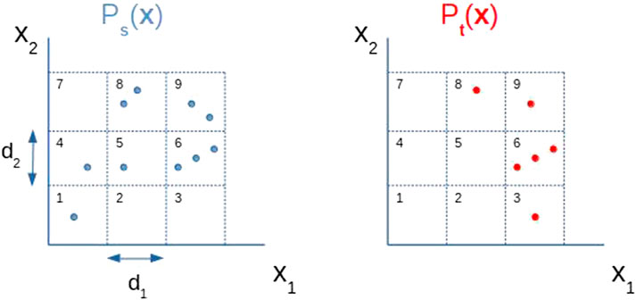
FIGURE 5. Discretization of a two dimensional random variable x = (x₁, x₂). The values of discretization steps d₁ and d₂ determine the size of each rectangle. Now, $B(P_s,P_t)=-\ln {\sum }_{i=1}^9\sqrt{p_i^s{p}_i^t}$, where p_i is a probability of x belonging to rectangle i (i.e. $p_3^t=1/6$).

Apart from BD, there are other popular methods to calculate the statistical distance (or similarity between distributions) such as Mahalanobis distance (Mahalanobis, 1936), Kolmogorov-Smirnov test (Simard and L’Ecuyer, 2011), or Jensen-Shannon divergence (Lin, 1991). However, Mahalanobis distance calculates the distance between a point and a distribution, the Kolmogorov-Smirnov test works with one-dimensional random variables, and Jensen-Shannon divergence requires that, after discretizing the input space, the same hyper-cubes from both distributions cannot be both empty $(p_i^s=p_i^t=0)$.

2.3 Programming environment

In this research, two programming environments were used: data preprocessing and analyses were conducted using the R software environment (RCoreTeam, 2013); models were built using the Python PyTorch (Paszke et al., 2019) and ScikitLearn (Pedregosa et al., 2011) libraries. The code and the datasets used for the experiments can be downloaded from the GitHub repository [SocTransferLearning].

3 Experiments and results

The evaluation of the proposed TL-based arable cropland SOC estimation model has been conducted in a leave-one-country-out procedure on a LUCAS-12 data set. For cropland samples in each country (12 target domains), we built two estimation models: classical ML, and TL. Both models were trained on soil samples obtained by merging data from the remaining 11 countries in two different experimental settings: 1) source domain contained soil samples only from cropland class areas, and 2) source domain contained samples only from grassland class areas.

3.1 Training the proposed transfer learning model

The proposed TL model is trained in two phases. In the first phase, a neural network classifier (Aggarwal, 2018) is trained to distinguish between the source and the target domain samples. A two-layer feed-forward network uses a Rectified Linear Unit (ReLU) activation function in each of the five neurons in the hidden layer. The number of hidden neurons is equal to the number of inputs which is a common choice for models with few inputs. The output neuron performs the Sigmoid function. The network is trained to minimize the binary cross-entropy loss in a standard backpropagation procedure (Aggarwal, 2018). When trained, the network assigns the probabilities of each source sample belonging to the source class (P(δ = 1|x)). The assigned probabilities will be used in the next phase to modify the mean squared error loss of the regression model defined in Eq. 5 – note that the ratio $\frac{1}{P(\delta =1|\mathbf{x})}$, according to Eq. 6, estimates the probability ratio $\frac{P_t(\mathbf{x})}{P_s(\mathbf{x})}$.

In the second phase, the regression model is trained only with the samples from the source domain, using both geochemical and physical variables as the inputs and related SOC values as the outputs. The model uses a two-layer, feed-forward neural network with five hidden neurons and one linear output. The network is trained in a standard backpropagation procedure using the modified, previously explained, loss function. Optimal hyperparameters (learning rate, momentum, and the number of training epochs) for the classification and regression networks are found in a standard 5-fold cross-validation procedure (Aggarwal, 2018).

When performing the experiments, classical ML models are trained using only the second phase of TL training in which the ratio $\frac{P_t(\mathbf{x})}{P_s(\mathbf{x})}$ is set to one. The schematic display of the training process is shown in Figure 6.

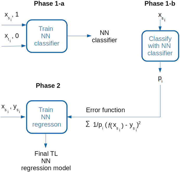
FIGURE 6. Two training phases for the TL model: In phase 1-a, a classifier is trained to distinguish between the source and the destination domain inputs; in phase 1-b, probabilities of source domain samples belonging to the source domain were calculated (p_i); in phase 2, a final regression model is trained only on the source domain labeled data, using the modified error function.

3.2 Model evaluation and discussion

The instance-based TL and classical models were compared using the normalized versions of Root Mean Squared Error (NRMSE) and Mean Absolute Error (NMAE), and Coefficient of Determination (R²):

Due to the quadratic term in the sum, Root Mean Squared Error is more sensitive to outliers (samples in which the difference between the real and the predicted value is large) than Mean Absolute Error. Both measures are normalized over the average value of the target variable (real SOC values in the target domain). Hence, different models trained for the same target domain can be relatively compared. The Coefficient of Determination shows how the trained model improves over the one that always predicts the average value of the target variable. If the trained model is perfect, then R² = 1; if the model always predicts the average value, like one would optimally do without learning, then R² = 0; for values of R² less than zero, the model is worse than one would achieve by always predicting the average value.

3.2.1 Experimental setting cropland-to-cropland

In this experimental setting, a source domain for each country consisted of the soil samples from the other 11 countries, covering only the cropland LC class. The target domain for each country consisted of the soil samples from its cropland LC class. In this manner, we tested the capability of TL to transfer knowledge from the global to the local geographical scale. The experimental results are shown in Table 2. In most of the considered countries, the TL model provides little better results in at least one performance measure. In the case of Austria, Germany, Greece, and Italy, there is no improvement in any of those measures, while in the United Kingdom and Poland all measures are slightly improved. The only measure that is slightly worse is R² for the Czech Republic, indicating that the proposed approach is at least as good as the classical one.

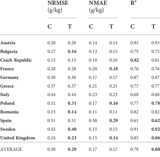
TABLE 2. Comparing classical (C), and transfer learning (T) approach in a Cropland-to-Cropland setting: normalized RMSE and MAE (lower is better), and R² (higher is better).

3.2.2 Experimental setting grassland-to-cropland

In this experimental setting, a source domain for each country consisted of the soil samples from the other 11 countries, covering only the grassland LC class. As in the previous experimental setting, the target domain for each country consisted of the soil samples from its cropland LC class. Hence, we tested the capability of TL to transfer knowledge from both global-to-local geographical scales and different, but related LC classes at the same time. The experimental results are shown in Table 3. The improvement in at least one of the measures was present in all the countries except for Sweden. In the case of Bulgaria, France, Germany, Italy, Poland, Romania, and Spain, all measures are improved. These improvements are significantly bigger than in the cropland-to-cropland experimental setting. For Spain the improvement is higher than 10% for each measure.

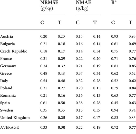
TABLE 3. Comparing classical (C), and transfer learning (T) approach in a Grassland-to-Cropland setting: normalized RMSE and MAE (lower is better), and R² (higher is better), indicate the benefits of the proposed TL approach.

3.2.3 Discussion

As can be seen from Tables 2 and 3, the average improvements of the proposed cropland SOC estimation model depend on the type of the source domain. While the improvement of a global-to-local geographical transfer of knowledge is negligible for the Cropland-to-Cropland case, a global-to-local transfer across land cover classes yields significant improvement for the Grassland-to-Cropland case. In all cases, NRMSE is higher than NMAE since NMAE is more robust to the outliers in the estimation process. All error measures are lower when the regression models are trained on the labeled cropland samples, which are naturally expected. However, when trained on the labeled grassland samples using a TL approach, the model can get close to the more natural model trained on the labeled cropland samples—classic Cropland-to-Cropland vs TL Grassland-to-Cropland: 0.30 vs 0.30 for average NRMSE; 0.17 vs 0.19 for average NMAE; 0.77 vs 0.79 for average R².

To explain the improved performance of the TL model compared to its classical counterpart for most target countries, we calculated the Bhattacharyya distance (BD) between the source and the target domain distributions in both experimental settings. How the distance (overlap) between the distributions affects the achieved improvement can be seen in Table 4. The benefits of TL over the classical approach for a particular country are more expressed if the distance between the source and the target domain distribution is greater. The transfer of SOC-related knowledge from the grassland to the cropland LC class achieves much better results (the central part of Table 4) than the transfer from the global to the local cropland LC class (the left part of Table 4). This result is expected since the instance-based TL model can benefit if the source and the destination input distributions are different enough so that there will be something to transfer—see Definition 2 in Section 2.2.1. If the distributions are almost identical, as in the case with the Cropland-to-Cropland setting, then the transferred knowledge is minimal.

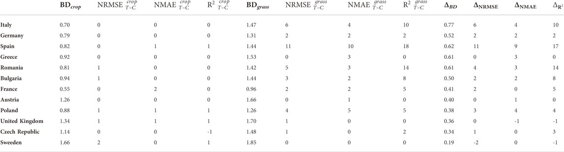
TABLE 4. Comparing the distance between source and target input distributions per each country and the improvement of the TL model over the classical model: BD_s - BD between a source domain s ∈{crop, grass} and a cropland target domain distributions per each country; ${\mathrm{M}}_{T-C}^s$ - the percentual improvement of performance metric M when a TL model is built on a source domain s; Δ_BD - increase in BD distance (BD_grass − BD_crop); Δ_M - the improvement in M of the TL model over the classical model when the transfer is conducted from the grassland source domain, compared to the cropland source domain $({\text{M}}_{T-C}^{\mathit{grass}}-{\text{M}}_{T-C}^{\mathit{crop}})$.

In the right part of Table 4, a relationship between the increase in distance for a particular country (Δ_BD = BD_grass − BD_crop) and the increase in performance M improvement of a TL model over the associated classical model $({\mathrm{\Delta }}_{\text{M}}={\text{M}}_{T-C}^{\mathit{grass}}-{\text{M}}_{T-C}^{\mathit{crop}})$ is shown. One can see that the higher values of Δ_BD correspond to higher values of Δ_M. This conclusion is confirmed by a calculated Pearson correlation coefficient between those two values: for Δ_NRMSE - 0.67 (p-value 0.02); for Δ_NMAE - 0.65 (p-value 0.02); for ${\mathrm{\Delta }}_{{\text{R}}^2}$ - 0.65 (p-value 0.02).

Despite the same range for corresponding variables values and discretization steps used when calculating distances between different domains, distances placed in different rows of Table 4 could not be simply compared due to a different number of cropland soil samples in a particular country.

4 Conclusion

Considering the importance of SOC in the overall terrestrial ecosystem, its estimation is a topic that occupied many researchers from the field of soil science. SOC estimation from geochemical and physical soil parameters in arable land is significant because of its permanent reduction due to tillage activities and climate changes and as a vital element for soil quality and fertility. In this study, we did not consider the classical ML models by themselves, which is the most often topic of recently published works in this area of research, but the possibility of upgrading these models using a transfer learning approach. The proposed TL methodology could be used to generate PTFs for target domains with described samples and unknown related PTF outputs if the described samples with known related PTF outputs from a different geographic or similar land class source domain are available. The assumption for the proposed methodology is that the source and the target distributions of samples are overlapping. In the case of equal distributions, a TL and a classical ML approach would be the same. If the distributions are totally different, then both classical ML and TL approaches would be inappropriate.

The proposed instance-based TL method improved SOC estimation in cropland areas of different target countries by transferring SOC-related knowledge from two global source domains: European cropland and European grassland (both data sets derived from the LUCAS 2015 survey). In both cases, an improvement over the classical ML-based model was evident. However, the benefit of applying TL was more significant when transferring from a different but related land cover class (grassland to cropland), which is in accordance with the starting assumption that the source and the target domain data come from different, but overlapping probability distributions. The effects of TL per particular country were different and could be further analyzed. The analysis should include expert knowledge about specific pedological patterns, climatic factors, and commonly applied agrotechnical practices. Nevertheless, the application of instance-based TL almost always outperformed its classical counterpart, and it could be recommended whenever additional soil data are available.

Instead of transferring knowledge from the global to the local domain, future research will investigate the efficiency of the proposed TL methodology in the inverse direction. Continuation of the study will be to examine the extrapolation of the information from detailed measured small to sparsely sampled larger areas (see Malone et al. (2016)). The other future research will include the additional covariates like climatic and remote sensing data from Sentinel satellite missions.

Data availability statement

The code and the datasets used for the experiments in this study can be downloaded from the GitHub repository [SocTransferLearning].

Author contributions

All coauthors PB, MK, and BB contributed to the conception and design of the study. PB organized the database. All coauthors PB, MK, and BB equally contributed to all aspects of the research and manuscript preparation and approved it for publication.

Funding

This research was funded by the Science Fund of the Republic of Serbia - Program for Development of Projects in the Field of Artificial Intelligence, grant number 6527073 (project acronym CERES).

Acknowledgments

The LUCAS topsoil dataset used in this work was made available by the European Commission through the European Soil Data Centre managed by the Joint Research Centre (JRC).

Conflict of interest

The authors declare that the research was conducted in the absence of any commercial or financial relationships that could be construed as a potential conflict of interest.

Publisher’s note

All claims expressed in this article are solely those of the authors and do not necessarily represent those of their affiliated organizations, or those of the publisher, the editors and the reviewers. Any product that may be evaluated in this article, or claim that may be made by its manufacturer, is not guaranteed or endorsed by the publisher.

References

Benke, K., Norng, S., Robinson, N., Chia, K., Rees, D., and Hopley, J. (2020). Development of pedotransfer functions by machine learning for prediction of soil electrical conductivity and organic carbon content. Geoderma 366, 114210. doi:10.1016/j.geoderma.2020.114210
Benos, L., Tagarakis, A. C., Dolias, G., Berruto, R., Kateris, D., and Bochtis, D. (2021). Machine learning in agriculture: A comprehensive updated review. Sensors 21, 3758. doi:10.3390/s21113758
Bhattacharyya, A. K. (1946). On a measure of divergence between two multinomial populations. Sankhyā Indian J. Statistics 7, 401–406.
Bouasria, A., Ibno, N. K., Rahimi, A., Ettachfini, E. M., and Rerhou, B. (2022). Evaluation of landsat 8 image pansharpening in estimating soil organic matter using multiple linear regression and artificial neural networks. Geo-spatial Inf. Sci., 1–12. doi:10.1080/10095020.2022.2026743
Bouma, J. (1989). “Using soil survey data for quantitative land evaluation,” in Advances in soil science (Springer), 177–213.
Bruhwiler, L., Michalak, A., Birdsey, R., Fisher, J., Houghton, R., Huntzinger, D., et al. (2018). “Overview of the global carbon cycle” in Second state of the carbon cycle report (SOCCR2): A sustained assessment report global change research program, 42–70.
Estévez, V., Beucher, A., Mattbäck, S., Boman, A., Auri, J., Björk, K.-M., et al. (2022). Machine learning techniques for acid sulfate soil mapping in southeastern Finland. Geoderma 406, 115446. doi:10.1016/j.geoderma.2021.115446
Gunarathna, M., Sakai, K., Nakandakari, T., Momii, K., and Kumari, M. (2019). Machine learning approaches to develop pedotransfer functions for tropical sri lankan soils. Water 11, 1940. doi:10.3390/w11091940
Hengl, T., de Jesus, J. M., Heuvelink, G., Gonzalez, M. R., Kilibarda, M., Blagotić, A., et al. (2017). Soilgrids250m: Global gridded soil information based on machine learning. PLoS One 12, e0169748. doi:10.1371/journal.pone.0169748
Heuvelink, G., Angelini, M., Poggio, L., Bai, Z., Batjes, N., van den Bosch, R., et al. (2021). Machine learning in space and time for modelling soil organic carbon change. Eur. J. Soil Sci. 72, 1607–1623. doi:10.1111/ejss.12998
Horwath, W. R., and Kuzyakov, Y. (2018). The potential for soils to mitigate climate change through carbon sequestration. Dev. Soil Sci. 35, 61–92. doi:10.1016/B978-0-444-63865-6.00003-X
Jones, A., Fernandez-Ugalde, O., and Scarpa, S. (2020). Lucas 2015 topsoil survey: Presentation of dataset and results. doi:10.2760/616084
Kovačević, M., Bajat, B., and Gajić, B. (2010). Soil type classification and estimation of soil properties using support vector machines. Geoderma 154, 340–347. doi:10.1016/j.geoderma.2009.11.005
Kovačević, M., Bajat, B., Trivić, B., and Pavlović, R. (2009). “Geological units classification of multispectral images by using support vector machines”, in 2009 international conference on intelligent networking and collaborative systems (ieee), 267–272.
Lin, J. (1991). Divergence measures based on the shannon entropy. IEEE Trans. Inf. Theory 37, 145–151. doi:10.1109/18.61115
Liu, L., Ji, M., and Buchroithner, M. (2018). Transfer learning for soil spectroscopy based on convolutional neural networks and its application in soil clay content mapping using hyperspectral imagery. Sensors 18, 3169. doi:10.3390/s18093169
Ludwig, M., Bahlmann, J., Pebesma, E., and Meyer, H. (2022). Developing transferable spatial prediction models: a case study of satellite based landcover mapping. Int. Arch. Photogramm. Remote Sens. Spat. Inf. Sci. 43, 135–141. doi:10.5194/isprs-archives-xliii-b3-2022-135-2022
Mahalanobis, P. C. (1936). On the generalised distance in statistics. Proc. Natl. Inst. Sci. India 2, 49–55.
Mahmood, A., Singh, S. K., and Tiwari, A. K. (2022a). Pre-trained deep learning-based classification of jujube fruits according to their maturity level. Neural comput. Appl. 34, 13925–13935. doi:10.1007/s00521-022-07213-5
Mahmood, A., Tiwari, A. K., Singh, S. K., and Udmale, S. S. (2022b). Contemporary machine learning applications in agriculture: Quo vadis? Concurrency Comput. 34, e6940. doi:10.1002/cpe.6940
Mallavan, B., Minasny, B., and McBratney, A. (2010). “Homosoil, a methodology for quantitative extrapolation of soil information across the globe,” in Digital soil mapping (Dordrecht: Springer), 137–150.
Malone, B. P., Jha, S. K., Minasny, B., and McBratney, A. B. (2016). Comparing regression-based digital soil mapping and multiple-point geostatistics for the spatial extrapolation of soil data. Geoderma 262, 243–253. doi:10.1016/j.geoderma.2015.08.037
McBratney, A. B., Minasny, B., Cattle, S. R., and Vervoort, W. R. (2002). From pedotransfer functions to soil inference systems. Geoderma 109, 41–73. doi:10.1016/s0016-7061(02)00139-8
McBratney, A., Odeh, I., Bishop, T., Dunbar, M., and Shatar, T. (2000). An overview of pedometric techniques for use in soil survey. Geoderma 97, 293–327. doi:10.1016/s0016-7061(00)00043-4
McBratney, A., Santos, M., and Minasny, B. (2003). On digital soil mapping. Geoderma 117, 3–52. doi:10.1016/s0016-7061(03)00223-4
McBratney, A., and Webster, R. (1983). Optimal interpolation and isarithmic mapping of soil properties: V. co-regionalization and multiple sampling strategy. J. Soil Sci. 34, 137–162. doi:10.1111/j.1365-2389.1983.tb00820.x
Meyer, H., and Pebesma, E. (2021). Predicting into unknown space? estimating the area of applicability of spatial prediction models. Methods Ecol. Evol. 12, 1620–1633. doi:10.1111/2041-210x.13650
Niu, X., Liu, C., Jia, X., and Zhu, J. (2021). Changing soil organic carbon with land use and management practices in a thousand-year cultivation region. Agric. Ecosyst. Environ. 322, 107639. doi:10.1016/j.agee.2021.107639
Obalum, S., Chibuike, G., Peth, S., and Ouyang, Y. (2017). Soil organic matter as sole indicator of soil degradation. Environ. Monit. Assess. 189, 1–19. doi:10.1007/s10661-017-5881-y
Orgiazzi, A., Ballabio, C., Panagos, P., Jones, A., and Fernández-Ugalde, O. (2018). Lucas soil, the largest expandable soil dataset for Europe: a review. Eur. J. Soil Sci. 69, 140–153. doi:10.1111/ejss.12499
Padarian, J., Minasny, B., and McBratney, A. (2020). Machine learning and soil sciences: A review aided by machine learning tools. Soil 6, 35–52. doi:10.5194/soil-6-35-2020
Padarian, J., Minasny, B., and McBratney, A. (2019). Transfer learning to localise a continental soil vis-nir calibration model. Geoderma 340, 279–288. doi:10.1016/j.geoderma.2019.01.009
Pan, S. J., and Yang, Q. (2010). A survey on transfer learning. IEEE Trans. Knowl. Data Eng. 22, 1345–1359. doi:10.1109/tkde.2009.191
Paszke, A., Gross, S., Massa, F., Lerer, A., Bradbury, J., Chanan, G., et al. (2019). “Pytorch: An imperative style, high-performance deep learning library,” in Advances in neural information processing systems 32. Editors H. Wallach, H. Larochelle, A. Beygelzimer, E. Fox, and R. Garnett (Red Hook, New York, US: Curran Associates, Inc.), 8024–8035.
Pedregosa, F., Varoquaux, G., Gramfort, A., Michel, V., Thirion, B., Grisel, O., et al. (2011). Scikit-learn: Machine learning in python. J. Mach. Learn. Res. 12, 2825–2830.
Ramcharan, A., Hengl, T., Beaudette, D., and Wills, S. (2017). A soil bulk density pedotransfer function based on machine learning: A case study with the ncss soil characterization database. Soil Sci. Soc. Am. J. 81, 1279–1287. doi:10.2136/sssaj2016.12.0421
Schmidt, M. W., Torn, M. S., Abiven, S., Dittmar, T., Guggenberger, G., Janssens, I. A., et al. (2011). Persistence of soil organic matter as an ecosystem property. Nature 478, 49–56. doi:10.1038/nature10386
Scull, P., Franklin, J., Chadwick, O., and McArthur, D. (2003). Predictive soil mapping: a review. Prog. Phys. Geogr. Earth Environ. 27, 171–197. doi:10.1191/0309133303pp366ra
Simard, R., and L’Ecuyer, P. (2011). Computing the two-sided kolmogorov-smirnov distribution. J. Stat. Softw. 39, 1–18. doi:10.18637/jss.v039.i11
Taghizadeh-Mehrjardi, R., Nabiollahi, K., and Kerry, R. (2016). Digital mapping of soil organic carbon at multiple depths using different data mining techniques in baneh region, iran. Geoderma 266, 98–110. doi:10.1016/j.geoderma.2015.12.003
Tan, C., Sun, F., Kong, T., Zhang, W., Yang, C., and Liu, C. (2018). “A survey on deep transfer learning,” in International conference on artificial neural networks (Springer), 270–279.
Wadoux, A. M.-C., Minasny, B., and McBratney, A. (2020). Machine learning for digital soil mapping: Applications, challenges and suggested solutions. Earth-Science Rev. 210, 103359. doi:10.1016/j.earscirev.2020.103359
Xiong, P., Long, C., Zhou, H., Battiston, R., Santis, A. D., Ouzounov, D., et al. (2021). Pre-earthquake ionospheric perturbation identification using cses data via transfer learning. Front. Environ. Sci. 514. doi:10.3389/fenvs.2021.779255
Yang, Q., Zhang, Y., Dai, W., and Pan, S. J. (2020). Transfer learning. Cambridge: Cambridge University Press.
Keywords: soil organic carbon, estimation, LUCAS data, transfer learning, Bhattasharyya distance, PTF
Citation: Bursać P, Kovačević M and Bajat B (2022) Instance-based transfer learning for soil organic carbon estimation. Front. Environ. Sci. 10:1003918. doi: 10.3389/fenvs.2022.1003918
Received: 26 July 2022; Accepted: 19 August 2022;
Published: 21 September 2022.
Edited by:
Daniela Businelli, University of Perugia, ItalyReviewed by:
Abdelkrim Bouasria, Chouaïb Doukkali University, MoroccoMirac Kilic, Adiyaman University, Turkey
Atif Mahmood, Dr. A.P.J Abdul Kalam Technical University, India
Balazs Grosz, Thünen Institut of Climate-Smart Agriculture, Germany
Copyright © 2022 Bursać, Kovačević and Bajat. This is an open-access article distributed under the terms of the Creative Commons Attribution License (CC BY). The use, distribution or reproduction in other forums is permitted, provided the original author(s) and the copyright owner(s) are credited and that the original publication in this journal is cited, in accordance with accepted academic practice. No use, distribution or reproduction is permitted which does not comply with these terms.
*Correspondence: Branislav Bajat, bajat@grf.bg.ac.rs