A Functional Data Analysis for Assessing the Impact of a Retrofitting in the Energy Performance of a Building

 , and
, and 
Abstract
:1. Introduction
2. Materials and Methods
2.1. Functional Data Analysis (FDA)
2.1.1. Functional Depths
2.1.2. Functional Test ANOVA (FANOVA)
2.1.3. Functional Strengths
- It is not mandatory to have prior information on data distribution. The study does not depend on or is not limited to certain distributions.
- The analysis takes into account time intervals as a unit. The sample analysed focusses on complete time units such as days, months or years.
- Analysis of homogeneity. The definition of outliers is different; it is based on the idea that, even though data do not surpass the cut-off, if they show constant deviations, they will be identified as outlier.
- Possibility of study trends. Besides calculating mean functions or detect outliers, it is also possible to study slight variations from the normal data behaviour of the data without outliers.
- Complete analysis of the time spectrum. Before this approach, most analyses were based on the values obtained in a given grid of discrete points. On the contrary, with FDA, it is possible to work with the entire time set in a continuous way.
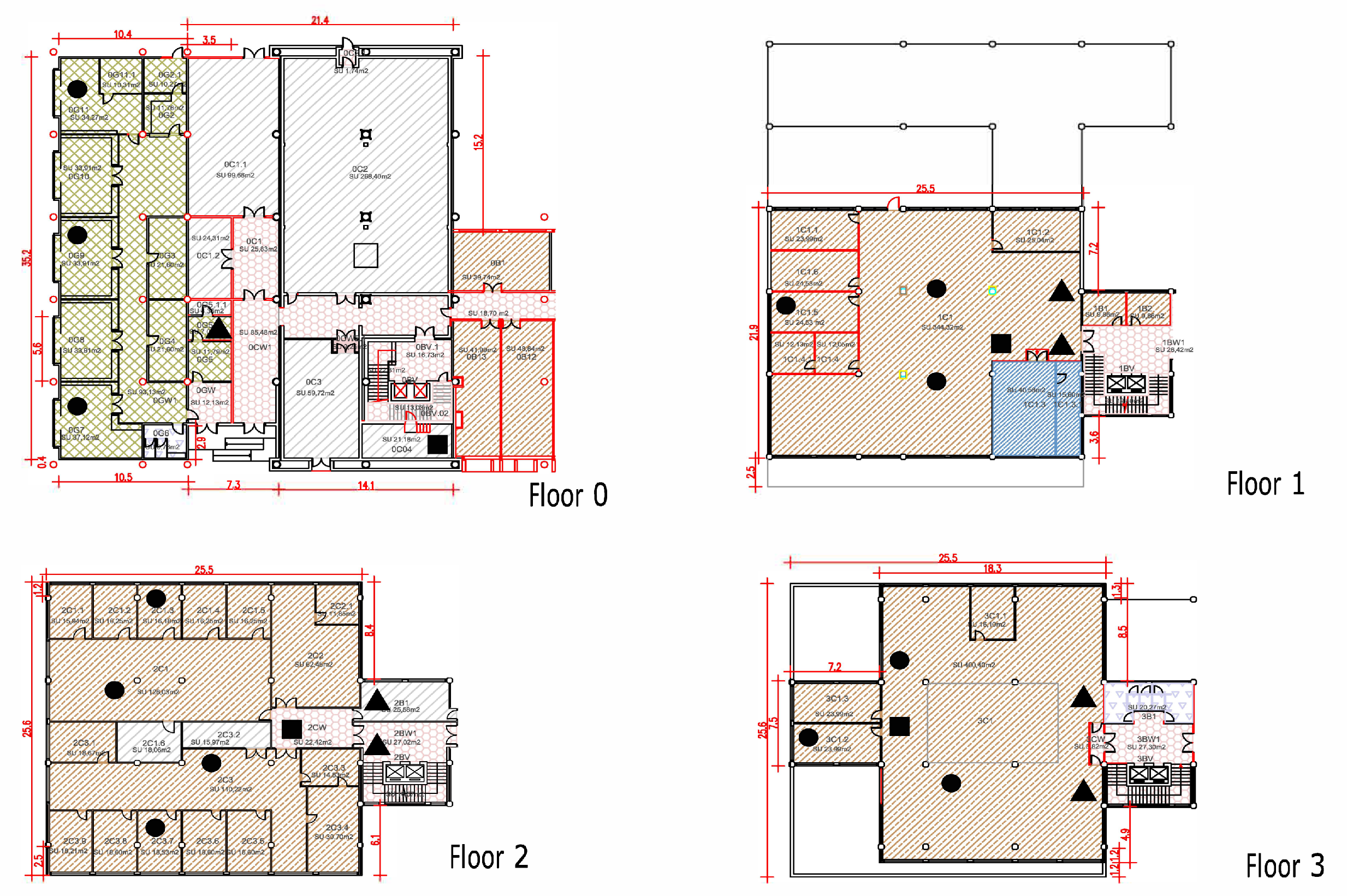
2.2. Building Description
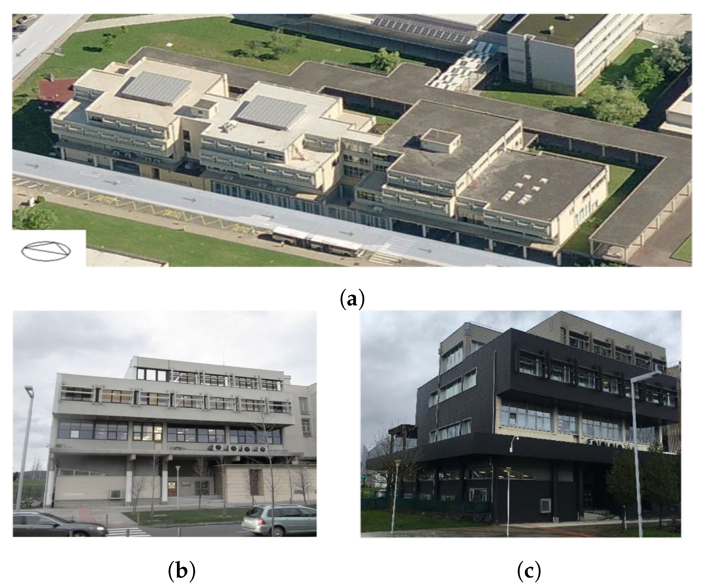
2.2.1. Building Description before Retrofitting
2.2.2. Building Description after Retrofitting
2.2.3. Monitoring Description of the Building
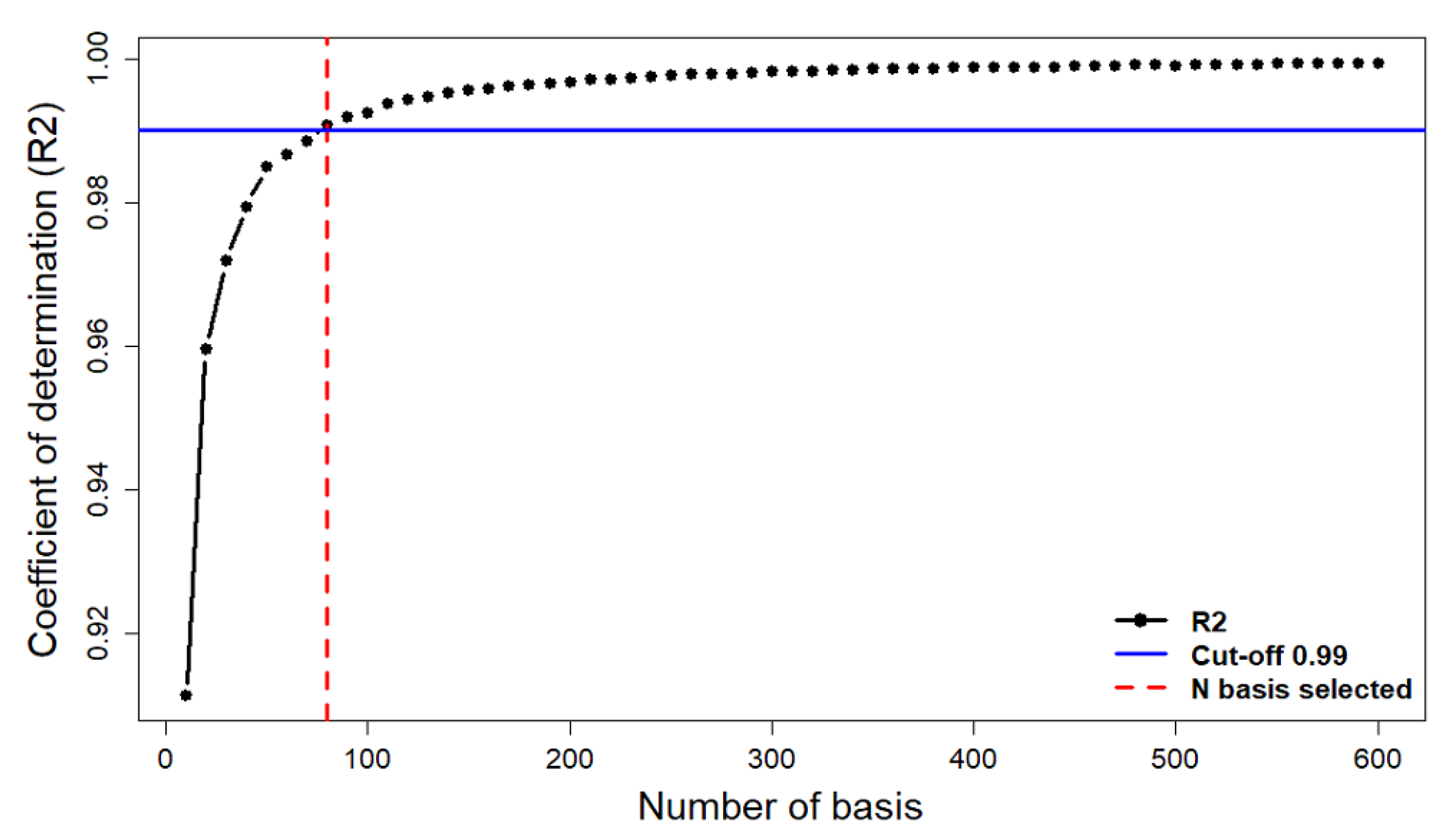
2.3. Pre-Processing Data
| Algorithm 1: Functional cleaning. |
| Input: Data divided in groups and the parameters: , , , . Output: Data without inappropriate days. 1 Transform the data to funcional format: 1440 minute data each day. 2 Searching for missing values (NAs). The daily limits are: NAs per day consecutive NAs per day 3 Delete the days that exceeded the daily limits. 4 Approximation, with an interpolation technique, of the remaining missing values. 5 Calculate the variability of every daily curve in the sample. 6 Delete the curves that:
|
3. Results and Discussion
3.1. Lighting Analysis
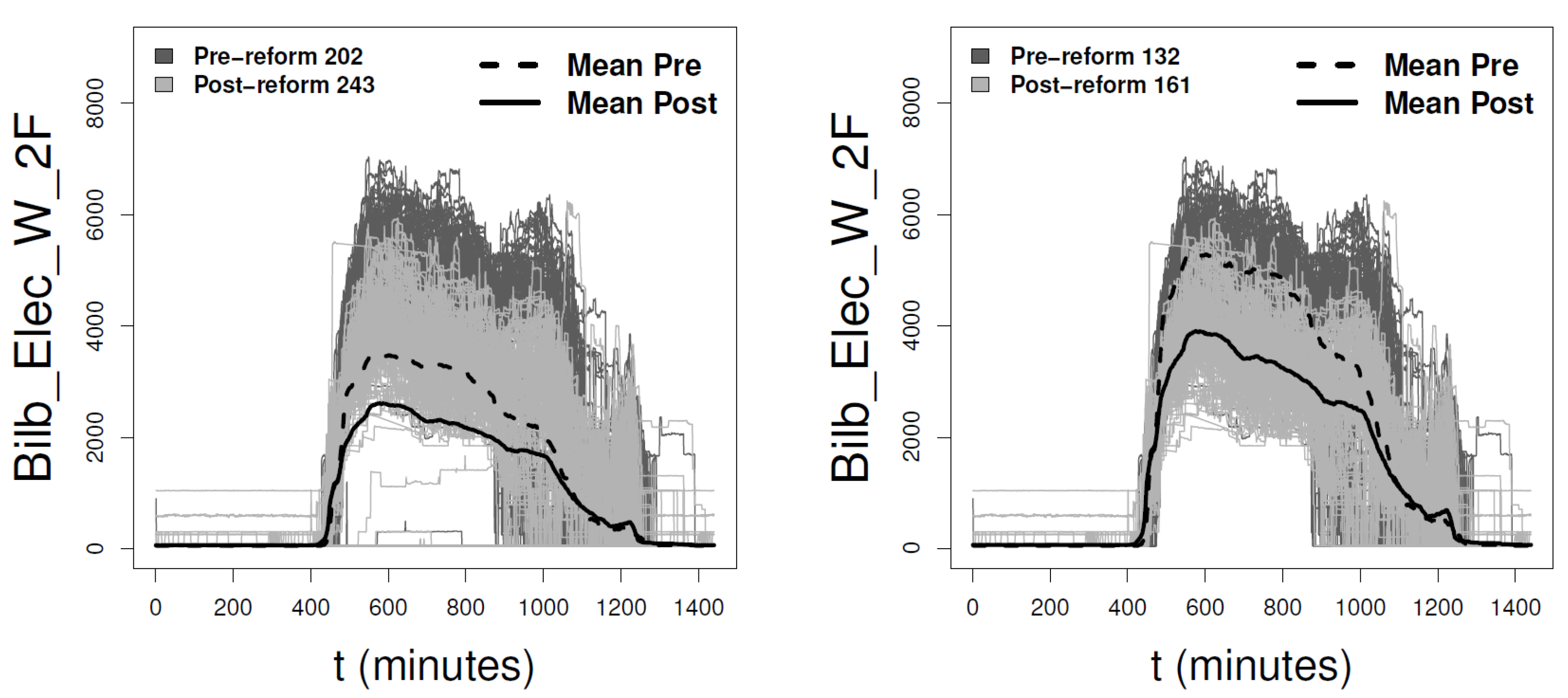
3.2. Heating Analysis
4. Conclusions
Author Contributions
Funding
Acknowledgments
Conflicts of Interest
References
- Foucquier, A.; Robert, S.; Suard, F.; Stéphan, L.; Jay, A. State of the art in building modelling and energy performances prediction: A review. Renew. Sustain. Energy Rev. 2013, 23, 272–288. [Google Scholar] [CrossRef] [Green Version]
- Energy Information Administration. International Energy Outlook 2019. Available online: https://www.eia.gov/ieo (accessed on 21 March 2020).
- RCP policy: Public health and health inequality. Every breath we take: The lifelong impact of air pollution. Royal College of Physicians (RCPCH). 2016. Available online: https://www.rcplondon.ac.uk/projects/outputs/every-breath-we-take-lifelong-impact-air-pollution (accessed on 21 March 2020).
- Wang, L.; Pereira, N.; Hung, Y. Air Pollution Control Engineering; Humana Press: New York, NY, USA, 2004. [Google Scholar]
- EEA. Air Quality in Europe; European Environmental Agency: Copenhagen, Denmark, 2019. [Google Scholar]
- Frances Bean, J.; Dorizas, V.; Bourdakis, E.; Staniaszek, D.; Pagliano, L.; Roscetti, A. Future-Proof Buildings for all Europeans—A Guide to Implement the Energy Performance of Buildings Directive; Buildings Performance Institute Europe (BPIE): Brussels, Belgium, 2019. [Google Scholar]
- Cabeza, L.F.; Rincón, L.; Vilariño, V.; Castell, A. Life cycle assessment (LCA) and life cycle energy analysis (LCEA) of buildings and the building sector: A review. Renew. Sustain. Energy Rev. 2014, 29, 394–416. [Google Scholar] [CrossRef]
- Santamouris, M.; Pavlou, C.; Doukas, P.; Mihalakakou, G.; Synnefa, A.; Hatzibiros, A.; Patargias, P. Investigating and analysing the energy and environmental performance of an experimental green roof system installed in a nursery school building in Athens, Greece. Energy 2007, 32, 1781–1788. [Google Scholar] [CrossRef]
- Chidiac, S.E.; Catania, E.J.; Morofky, E.; Foo, S. Effectiveness of single and multiple energy retrofit measures on the energy consumption of office buildings. Energy 2011, 36, 5037–5052. [Google Scholar] [CrossRef]
- Zmeureanu, R. Assessment of the energy savings due to the building retrofit. Build. Environ. 1990, 25, 95–103. [Google Scholar] [CrossRef]
- Asadi, E.; Da Silva, M.G.; Antunes, C.H.; Dias, L. Multi-objective optimization for building retrofit strategies: A model and an application. Energy Build. 2012, 44, 81–87. [Google Scholar] [CrossRef]
- Yalcintas, M. Energy-savings predictions for building-equipment retrofits. Energy Build. 2008, 40, 2111–2120. [Google Scholar] [CrossRef]
- Tobias, L.; Vavaroutsos, G. Retrofitting Buildings to be Green and Energy-Efficient: Optimizing Building Performance, Tenant Satisfaction, and financial Return; Urban Land Institute: Washington, DC, USA, 2012. [Google Scholar]
- Hamburg, A.; Kalamees, T. How well are energy performance objectives being achieved in renovated apartment buildings in Estonia? Energy Build. 2019, 199, 332–341. [Google Scholar] [CrossRef]
- Ardente, F.; Beccali, M.; Cellura, M.; Mistretta, M. Energy and environmental benefits in public buildings as a result of retrofit actions. Renew. Sustain. Energy Rev. 2011, 15, 460–470. [Google Scholar] [CrossRef]
- Mohammadpourkarbasi, H.; Sharples, S. Eco-retrofitting very old dwellings: Current and future energy and carbon performance for two UK cities, Plea 2013. In Proceedings of the 29th Conference, Munich, Germany, 10–12 September 2013. [Google Scholar]
- Beccali, M.; Cellura, M.; Fontana, M.; Longo, S.; Mistretta, M. Energy retrofit of a single-family house: Life cycle net energy saving and environmental benefits. Renew. Sustain. Energy Rev. 2013, 27, 283–293. [Google Scholar] [CrossRef]
- Famuyibo, A.A.; Duffy, A.; Strachan, P. Achieving a holistic view of the life cycle performance of existing dwellings. Build. Environ. 2013, 70, 90–101. [Google Scholar] [CrossRef] [Green Version]
- Ficco, G.; Iannetta, F.; Ianniello, E.; dAmbrosio Alfano, F.R.; DellIsola, M. U-value in situ measurement for energy diagnosis of existing buildings. Energy Build. 2015, 104, 108–121. [Google Scholar] [CrossRef]
- Uriarte, I.; Erkoreka, A.; Giraldo-Soto, C.; Martin, K.; Uriarte, A.; Eguia, P. Mathematical development of an average method for estimating the reduction of the Heat Loss Coefficient of an energetically retrofitted occupied office building. Energy Build. 2019, 192, 101–122. [Google Scholar] [CrossRef]
- Zavadskas, E.; Kaklaukas, A.; Turskis, Z.; Kalibatas, D. An approach to multi-attribute assessment of indoor environment before and after refurbishment of dwellings. J. Environ. Eng. Landsc. Manag. 2009, 17, 5–11. [Google Scholar] [CrossRef]
- Febrero, M.; Galeano, P.; Wenceslao, G. Outlier detection in functional data by depth measures, with application to identify abnormal NOx levels. Environmetrics 2008, 19, 331–345. [Google Scholar] [CrossRef]
- Horváth, L.; Kokoszka, P. Inference for Functional Data with Applications; Springer: Berlin/Heidelberg, Germany, 2012. [Google Scholar]
- Martínez, J.; Saavedra, A.; García, P.; Piñeiro, J.; Iglesias, C.; Taboada, J.; Sancho, J.; Pastor, J. Air quality parameters outliers detection using functional data analysis in the Langreo urban area (Northern Spain). Appl. Math. Comput. 2014, 241, 1–10. [Google Scholar] [CrossRef]
- Pi neiro, J.; Torres, J.; García, P.; Alonso, J.; Mu niz, C.; Taboada, J. Analysis and detection of functional outliers in waterquality parameters from different automated monitoring stationsin the Nalón River Basin (Northern Spain). Environ. Sci. Pollut. Res. 2015, 22, 387–396. [Google Scholar] [CrossRef]
- Martínez, J.; Pastor, J.; Sancho, J.; McNabola, A.; Martínez, M.; Gallagher, J. A functional data analysis approach for the detection of air pollution episodes and outliers: A case study in Dublin, Ireland. Mathematics 2020, 8, 225. [Google Scholar] [CrossRef] [Green Version]
- Sancho, J.; Martínez, J.; Pastor, J.; Taboada, J.; Piñeiro, J.; García Nieto, P. New methodology to determine air quality in urban areas based on runs rules for functional data. Atmos. Environ. 2014, 83, 185–192. [Google Scholar] [CrossRef]
- Sancho, J.; Iglesias, C.; Piñeiro, J.; Martínez, J.; Pastor, J.; Araújo, M.; Taboada, J. Study of water quality in a spanish river based on statistical process control and functional data analysis. Math. Geosci. 2016, 48, 163–186. [Google Scholar] [CrossRef]
- Iglesias, C.; Sancho, J.; Piñeiro, J.I.; Martínez, J.; Pastor, J.J.; Taboada, J. Shewhart-type control charts and functional data analysis for water quality analysis based on a global indicator. Desalin. Water Treat. 2016, 57, 2669–2684. [Google Scholar] [CrossRef]
- Dombeck, D.; Graziano, M.; Tank, D. Functional clustering of neurons in motor cortex determined by cellular resolution imaging in awake behaving mice. J. Neurosis. 2009, 29, 13751–13760. [Google Scholar] [CrossRef] [PubMed]
- Martínez, J.; Ordoñez, C.; Matìas, J.M.; Taboada, J. Determining noise in an aggregates plant using functional statistics. Hum. Ecol. Risk Assess. 2011, 17, 521–533. [Google Scholar] [CrossRef]
- Ordóñez, C.; Martínez, J.; Saavedra, A.; Mourelle, A. Intercomparison Exercise for Gases Emitted by a Cement Industry in Spain: A Functional Data Approach. J. Air Waste Manag. Assoc. 1995 2011, 61, 135–141. [Google Scholar] [CrossRef] [PubMed] [Green Version]
- Sancho, J.; Pastor, J.; Martínez, J.; García, M. Evaluation of Harmonic Variability in Electrical Power Systems through Statistical Control of Quality and Functional Data Analysis. In Procedia Engineering; The Manufacturing Engineering Society: Southfield, MI, USA, 2013; Volume 63, pp. 295–302. [Google Scholar] [CrossRef] [Green Version]
- Wu, D.; Huang, S.; Xin, J. Dynamic compensation for an infrared thermometer sensor using least-squares support vector regression (LSSVR) based functional link artificial neural networks (FLANN). Meas. Sci. Technol. 2008, 19, 105202.1–105202.6. [Google Scholar] [CrossRef]
- Ordoñez, C.; Martínez, J.; Cos Juez, J.; Sánchez Lasheras, F. Comparison of GPS observations made in a forestry setting using functional data analysis. Int. J. Comput. Math. 2012, 89, 402–408. [Google Scholar] [CrossRef]
- Müller, H.G.; Sen, R.; Stadtmüller, U. Functional data analysis for volatility. J. Econometr. 2011, 165, 233–245. [Google Scholar] [CrossRef] [Green Version]
- López, M.; Martínez, J.; Matías, J.M.; Taboada, J.; Vilán, J.A. Functional classification of ornamental stone using machine learning techniques. J. Comput. Appl. Math. 2010, 234, 1338–1345. [Google Scholar] [CrossRef] [Green Version]
- López, M.; Martínez, J.; Matías, J.M.; Taboada, J.; Vilán, J.A. Shape functional optimization with restrictions boosted with machine learning techniques. J. Comput. Appl. Math. 2010, 234, 2609–2615. [Google Scholar] [CrossRef] [Green Version]
- Flores, M.; Naya, S.; Fernández-Casal, R.; Zaragoza, S.; Raña, P.; Tarrío-Saavedra, J. Constructing a Control Chart Using Functional Data. Mathematics 2020, 8, 58. [Google Scholar] [CrossRef] [Green Version]
- Warmenhoven, J.; Harrison, A.; Robinson, M.A.; Vanrenterghem, J.; Bargary, N.; Smith, R.; Cobley, S.; Draper, C.; Donnelly, C.; Pataky, T. A force profile analysis comparison between functional data analysis, statistical parametric mapping and statistical non-parametric mapping in on-water single sculling. J. Sci. Med. Sport 2018, 21, 1100–1105. [Google Scholar] [CrossRef] [PubMed] [Green Version]
- Ordoñez, C.; Martínez, J.; Matías, J.M.; Reyes, A.N.; Rodríguez-Pérez, J.R. Functional statistical techniques applied to vine leaf water content determination. Math. Comput. Model. 2010, 52, 1116–1122. [Google Scholar] [CrossRef]
- Eisenhart, C. The Assumptions Underlying the Analysis of Variance. Int. Biometr. Soc. 1947, 3, 1–21. [Google Scholar] [CrossRef]
- Montgomery, D. Design and Analysis of Experiments, 8th ed.; John Wiley & Sons, Inc.: Hoboken, NJ, USA, 2013. [Google Scholar]
- Kotz, S.; Johnson, N.L. Breakthroughs in Statistics. Volume II. Methodology and Distribution; Springer: Berlin/Heidelberg, Germany, 1993; Volume 2. [Google Scholar]
- Vikneswaran. An R companion to “Experimental Design”; Vikneswaran: Duxbury, MA, USA, 2005. [Google Scholar]
- Crawley, M. The R Book, 2nd ed.; John Wiley & Sons: Hoboken, NJ, USA, 2013. [Google Scholar]
- Theodorsson-Norheim, E. Kruskal-Wallis test: BASIC computer program to perform nonparametric one-way analysis of variance and multiple comparisons on ranks of several independent samples. Comput. Meth. Prog. Biomed. 1986, 23, 57–62. [Google Scholar] [CrossRef]
- Ostertagová, E.; Ostertag, O.; Kovác, J. Methodology and application of the Kruskal-Wallis test. Mech. Mater. 2014, 611, 115–120. [Google Scholar] [CrossRef]
- Van Hecke, T. Power study of anova versus Kruskal Wallis test. Stat. Manag. Syst. 2012, 15, 241–247. [Google Scholar]
- Cuevas, A.; Febrero, M.; Fraiman, R. An anova test for functional data. Comput. Stat. Data Anal. 2004, 47, 111–122. [Google Scholar] [CrossRef]
- Tarrío-Saavedra, J.; Naya, S.; Francisco-Fernández, M.; Artiaga, R.; Lopez-Beceiro, J. Application of functional ANOVA to the study of thermal stability of micro–nano silica epoxy composites. Chemometr. Intell. Lab. Syst. 2011, 105, 114–124. [Google Scholar] [CrossRef]
- Kaufman, C.G.; Sain, S.R. Bayesian functional (ANOVA) modeling using Gaussian process prior distributions. Bayes. Anal. 2010, 5, 123–149. [Google Scholar] [CrossRef]
- Wang, J.L.; Chiou, J.M.; Müller, H.G. Functional Data Analysis. Ann. Rev. Stat. Appl. 2016, 3, 257–295. [Google Scholar] [CrossRef] [Green Version]
- Kramosil, I.; Michálek, J. Fuzzy metrics and statistical metric spaces. Kybernetika 1975, 11, 336–344. [Google Scholar]
- Ramsay, J.; Silverman, B. Applied Functional Data Analysis: Methods and Cae Studies; Springer: Berlin/Heidelberg, Germany, 2002. [Google Scholar]
- Walz, M.; Zebrowski, T.; Küchenmeister, J.; Busch, K. B-spline modal method: A polynomial approach compared to the Fourier modal method. Opt. Express 2013, 21, 14683–14697. [Google Scholar] [CrossRef] [PubMed] [Green Version]
- Muñiz, C.; García, P.; Alonso, J.; Torres, J.; Taboada, J. Detection of outliers in water quality monitoring samples using functional data analysis in San Esteban estuary (Northern Spain). Sci. Total Environ. 2012, 439, 54–61. [Google Scholar] [CrossRef] [PubMed]
- Martínez, J.; García, P.; Alejano, L.; Reyes, A. Detection of outliers in gas emissions from urban areas using functional data analysis. J. Hazard. Mater. 2011, 186, 144–149. [Google Scholar] [CrossRef]
- Fraiman, R.; Muniz, G. Trimmed means for functional data. TEST Off. J. Spanish Soc. Stat. Operat. Res. 2001, 10, 419–440. [Google Scholar] [CrossRef]
- Cuevas, A.; Febrero, M.; Fraiman, R. Robust estimationand classification for functional data via projection-based notions. Comput. Stat. 2007, 22, 481–496. [Google Scholar] [CrossRef]
- Cuevas, A.; Febrero, M.; Fraiman, R. On the use of bootstrap for estimating functions with functional data. Comput. Stat. Data Anal. 2006, 51, 1063–1074. [Google Scholar] [CrossRef]
- Léger, C.; Romano, J. Boostrap adaptive estimation. The trimmed-mean example. Can. J. Stat. 1990, 18, 297–314. [Google Scholar] [CrossRef]
- Hall, P.; Maesono, Y. A Weighted Bootstrap Approach to Bootstrap Iteration. J. R. Stat. Soc. Ser. B Stat. Methodol. 2000, 62, 137–144. [Google Scholar] [CrossRef]
- Millán-Roures, L.; Epifanio, I.; Martínez, V. Detection of Anomalies in Water Networks by Functional Data Analysis. Math. Problems Eng. 2018, 2018, 13. [Google Scholar] [CrossRef]
- Dette, H.; Derbort, S. Analysis of Variance un Non Parametric regression Models. J. Multivar. Anal. 2001, 76, 110–137. [Google Scholar] [CrossRef] [Green Version]
- Maldonado, Y.; Staniswalis, J.; Irwin, L.; Byers, D. A similarity analysis of curves. Can. J. Stat. 2002, 30, 373–381. [Google Scholar] [CrossRef]
- Cuesta-Albertos, J.A.; Febrero, M. A simple multiway ANOVA for functional data. TEST 2010, 19, 537–557. [Google Scholar] [CrossRef]
- Zhang, J.T. Analysis of Variance for Functional Data. In A Chapman & Hall Book; Press, C., Ed.; Taylor & Francis Group: Abingdon, UK, 2013; Chapter 5; p. 412. [Google Scholar]
- Erkoreka, A.; García, K.; Teres-Zubiaga, J.; Del Portillo, L. In-use office building energy characterization through basic monitoring and modelling. Energy Build. 2016, 119, 256–266. [Google Scholar] [CrossRef]


| Type of Measurement | Monitored Variable | Units | Sensor | |
|---|---|---|---|---|
| Indoor conditions | Illuminance | [LUX] | Siemens 5WG1 255-4AB12 | |
| Temperature | [°C] | ARCUS SK04-S8-CO2-TF | ||
| Electrical Consumption | Before retrofitting | Lighting + elec. equipment | W | Power meters ABB EM/S and ABB a41/43 per floor |
| After retrofitting | Lighting | W | ||
| Ventilation + elec. equipment | W | Power meters ABB EM/S and ABB a41/43 per floor | ||
| Heating consumption | Thermal energy of the heating water | W | Calorimeter: Kamstrup Multical 602 and ZENNER Zelsius (DN20) | |
| Electrical Consumption | |||||||||||
|---|---|---|---|---|---|---|---|---|---|---|---|
| Vectorial Analysis | Functional Analysis | ||||||||||
| panova | pkruskal | Dvec (W) | △Var | Savings | pfanova | Dfunc (W) | Ddist | △Var | Savings | R2 | |
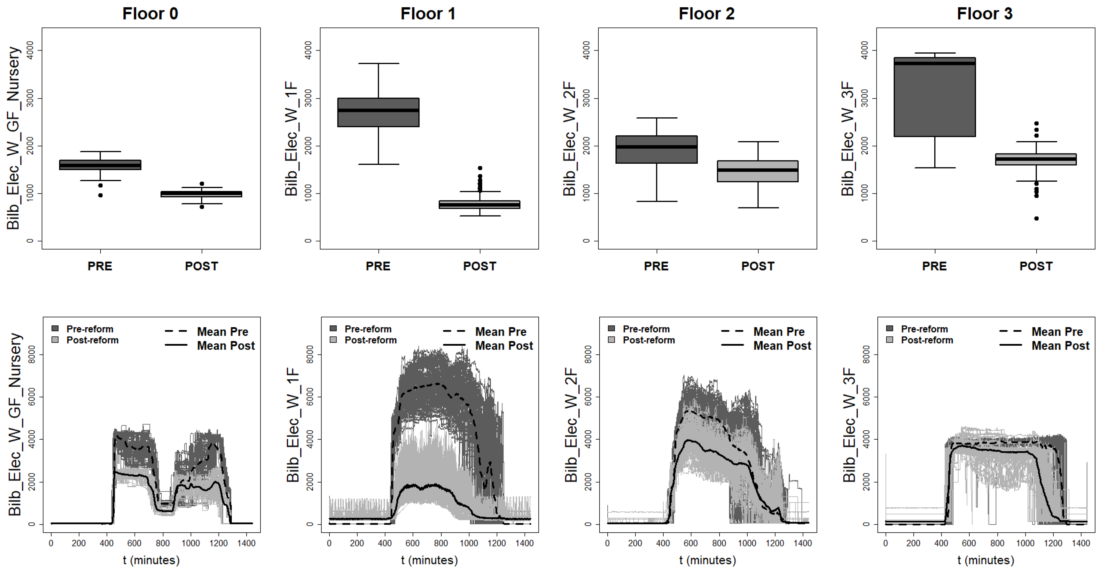
| Floor 0 | ≈0 | ≈0 | −587.48 | −72.63% | 36.96% | ≈0 | −609.69 | 34536.02 | −71.80 % | 38.11% | 0.9909 |
| Floor 1 | ≈0 | ≈0 | −1987.68 | −94.47% | 72.68% | ≈0 | −2032.31 | 116400.04 | −89.54% | 73.15% | 0.9903 |
| Floor 2 | ≈0 | ≈0 | −489.05 | −43.49% | 24.83% | ≈0 | −434.68 | 29537.58 | −55.54% | 22.50% | 0.9929 |
| Floor 3 | ≈0 | ≈0 | −2004.80 | −95.32% | 53.82% | ≈0 | −400.82 | 35603.07 | + 17.29% | 18.18% | 0.9915 |
| Illuminance | |||||||||
|---|---|---|---|---|---|---|---|---|---|
| Vectorial Analysis | Functional Analysis | ||||||||
| panova | pkruskal | Dvec (lx) | △Var | pfanova | Dfunc (lx) | Ddist | △Var | R2 | |
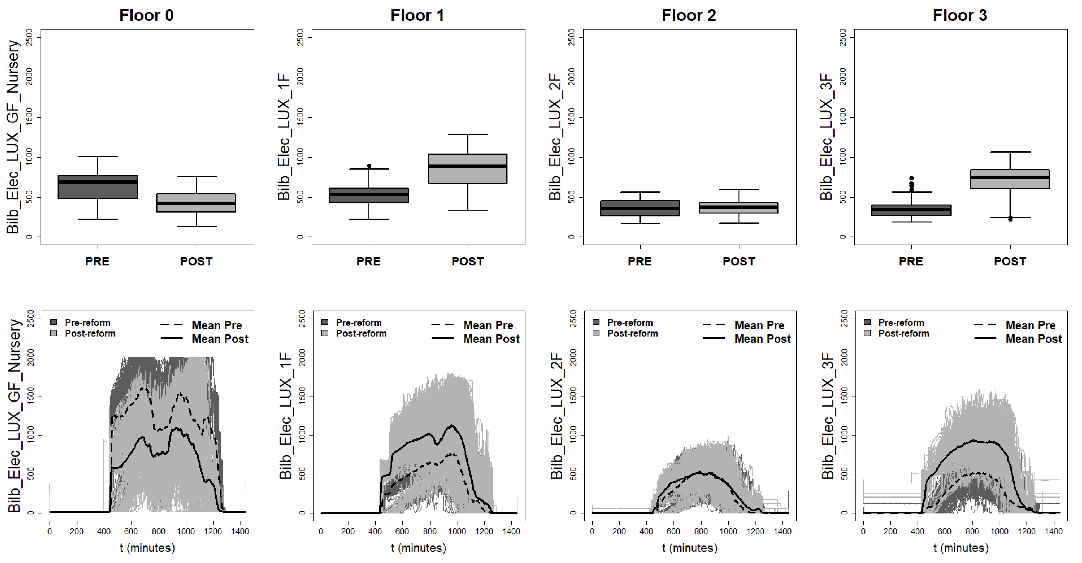
| Floor 0 | ≈0 | ≈0 | −266.22 | −42.27% | ≈0 | −286.81 | 15274.23 | −12.51% | 0.9909 |
| Floor 1 | ≈0 | ≈0 | +356.12 | +62.88% | ≈0 | +174.78 | 9379.46 | +59.44% | 0.9913 |
| Floor 2 | 0.217 | 0.278 | +9.46 | −27.78% | ≈0 | +23.33 | 1608.27 | −9.29% | 0.9904 |
| Floor 3 | ≈0 | ≈0 | +414.86 | +81.24% | ≈0 | +204.32 | 11140.84 | +66.30% | 0.9914 |
| Heating Demand | |||||||||||
|---|---|---|---|---|---|---|---|---|---|---|---|
| Vectorial Analysis | Functional Analysis | ||||||||||
| panova | pkruskal | Dvec (W) | △Var | Savings | pfanova | Dfunc (W) | Ddist | △Var | Savings | R2 | |
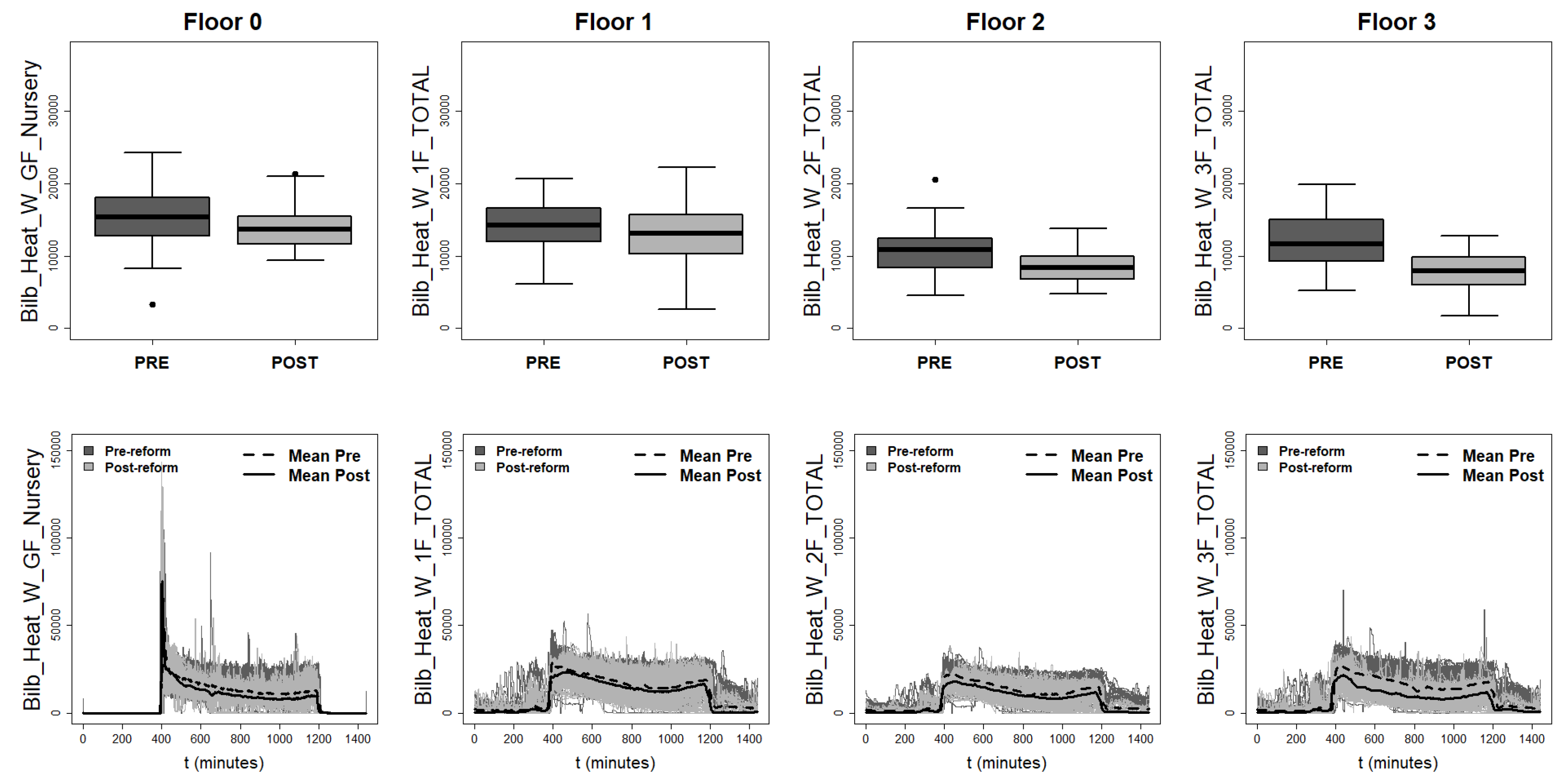
| Floor 0 | 1.761 × 10⁻⁶ | 7.047 × 10⁻⁶ | −1838.12 | −35.68% | 11.86% | ≈0 | −1455.83 | 158722.42 | −30.66% | 17.36% | 0.9901 |
| Floor 1 | 0.018 | 0.02 | −1057.67 | +24.71% | 7.46% | ≈0 | −1975.15 | 95981.90 | −23.89% | 16.97% | 0.9908 |
| Floor 2 | ≈0 | ≈0 | −2457.87 | −43.99% | 22.73% | ≈0 | −2158 | 96002.01 | −43.48% | 23.60% | 0.9914 |
| Floor 3 | ≈0 | ≈0 | −3667.06 | −60.22% | 31.49% | ≈0 | −3917.87 | 185968.48 | −51.68% | 35.51% | 0.9911 |
| Indoor Temperatures | |||||||||
|---|---|---|---|---|---|---|---|---|---|
| Vectorial Analysis | Functional Analysis | ||||||||
| panova | pkruskal | Dvec (W) | △Var | pfanova | Dfunc (W) | Ddist | △Var | R2 | |
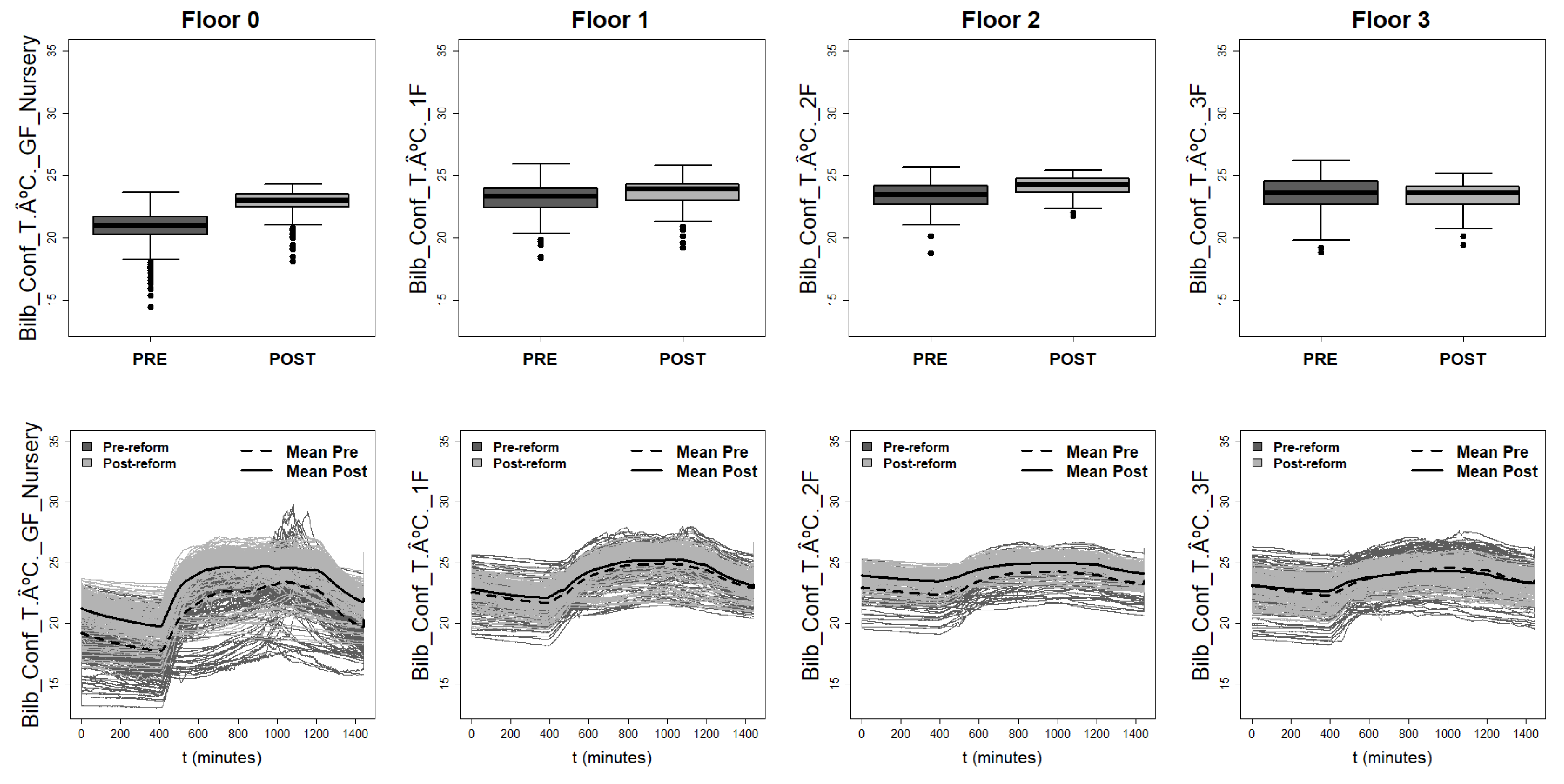
| Floor 0 | ≈0 | ≈0 | +1.92 | −62.75% | ≈0 | +1.95 | 75.09 | −40.10% | 0.9918 |
| Floor 1 | 0.001 | 0.004 | +0.55 | −45.33% | ≈0 | +0.35 | 13.43 | −37.77% | 0.9970 |
| Floor 2 | ≈0 | ≈0 | +0.76 | −53.31% | ≈0 | +0.92 | 35.29 | −60.68% | 0.9976 |
| Floor 3 | 0.39 | 0.274 | −0.072 | −50.65% | 0.17 | +0.002 | 7.97 | −63.15% | 0.9959 |
© 2020 by the authors. Licensee MDPI, Basel, Switzerland. This article is an open access article distributed under the terms and conditions of the Creative Commons Attribution (CC BY) license (http://creativecommons.org/licenses/by/4.0/).
Share and Cite
Martínez Comesaña, M.; Martínez Mariño, S.; Eguía Oller, P.; Granada Álvarez, E.; Erkoreka González, A. A Functional Data Analysis for Assessing the Impact of a Retrofitting in the Energy Performance of a Building. Mathematics 2020, 8, 547. https://doi.org/10.3390/math8040547
Martínez Comesaña M, Martínez Mariño S, Eguía Oller P, Granada Álvarez E, Erkoreka González A. A Functional Data Analysis for Assessing the Impact of a Retrofitting in the Energy Performance of a Building. Mathematics. 2020; 8(4):547. https://doi.org/10.3390/math8040547
Chicago/Turabian StyleMartínez Comesaña, Miguel, Sandra Martínez Mariño, Pablo Eguía Oller, Enrique Granada Álvarez, and Aitor Erkoreka González. 2020. "A Functional Data Analysis for Assessing the Impact of a Retrofitting in the Energy Performance of a Building" Mathematics 8, no. 4: 547. https://doi.org/10.3390/math8040547